A weighted random survival forest

Abstract

A weighted random survival forest is presented in the paper. It can be regarded as a modification of the random forest improving its performance. The main idea underlying the proposed model is to replace the standard procedure of averaging used for estimation of the random survival forest hazard function by weighted avaraging where the weights are assigned to every tree and can be veiwed as training paremeters which are computed in an optimal way by solving a standard quadratic optimization problem maximizing Harrell’s C-index. Numerical examples with real data illustrate the outperformance of the proposed model in comparison with the original random survival forest.

Keywords: random forest, decision tree, quadratic programming, survival analysis, Harrell’s C-index, cumulative hazard function.

1 Introduction

A lot of computer aided diagnosis (CAD) systems have been developed in order to provide successful detection of a disease and to facilitate making decision to start treatment process at early stage. Most CAD systems aim to detect a disease or its features. However, there are a few systems which take into account survival aspects of a patient especially of a cancer patient. Two reasons of such the situation can be pointed out. First, CAD systems taking into account survival aspects require the corresponding datasets which are mainly lack or of a small size nowadays. Second, CAD systems have to handle data with censored observations. This peculiarity may significantly complicate training process, and it requires special methods for dealing with censored data. A large amount of structured data, which has been recorded about patients, their peculiarities, do not take into account survival aspects. Therefore, it is topical to develop models which could efficiently process the available survival datasets in order to be an element of CAD systems.

A basis for such the models may be survival analysis or time-to-event analysis which can be regarded as a fundamental tool which is used in many applied areas. One of the most important areas is the medical research where survival models are widely used to evaluate the significance of prognostic variables in outcomes such as death or cancer recurrence and subsequently inform patients of their treatment options [34]. The datasets used in the survival analysis or just the survival data differ from many datasets by the fact that time to event of interest for a part of observations or instances is unknown because the event might not have happened during the period of study [49]. If the observed survival time is less than or equal to the true survival time, then we have a special case of censoring data called right-censoring data. Other special cases are left-censoring and interval censoring observations [65]. However, right-censoring is the most common case in many applications [24]. Without loss of generality, we describe the survival models mainly in the medical application terms below, i.e., instances will be called patients.

The survival models can be divided into three parts: parametric, nonparametric and semiparametric. It is assumed in parametric models that the type of the probability distribution of survival times is known, for example, the exponential, Weibull, normal, gamma distributions. As pointed out by Lee and Wang [41], nonparametric or distribution-free models are less efficient than parametric methods when survival times follow a theoretical distribution and more efficient when no suitable theoretical distributions are known. They can be used to analyze survival data before attempting to fit a theoretical distribution. One of the simplest survivor models is the Kaplan-Meier estimator which is a non-parametric model used to compute the survival function of a homogeneous data set. In other words, the model does not take into account the fact that the instances may differ by their features. A few critical features of the Kaplan-Meier model are considered in [41, Chapter 4, Page 76]. Nevertheless, the Kaplan-Meier model provides a simple way to compute the survival function of patients.

A popular regression model for the analysis of survival data is the well-known Cox proportional hazards model, which is a semi-parametric model that calculates the effects of observed covariates on the risk of an event occurring, for example, the death or failure [12]. The Cox model is the most commonly used regression analysis approach for survival data among semi-parametric survival models. The model does not require knowledge of the underlying distribution. It differs significantly from other methods since it is built on the proportional hazards assumption and employs partial likelihood for parameter estimation. The proportional hazards assumption in the Cox model means that different patients have hazard functions that are proportional, i.e., the ratio of the hazard functions for two patients with different prognostic factors or covariates is a constant and does not vary with time. In other words, the ratio of the risk of dying of two patients is the same no matter how long they survive [41, Chapter 12]. The model assumes that a patient’s log-risk of failure is a linear combination of the patient’s covariates. This assumption is referred to as the linear proportional hazards condition. It is interesting to note that the Cox model is semi-parametric in the sense that it can be factored into a parametric part consisting of a regression parameter vector associated with the covariates and a non-parametric part that can be left completely unspecified [15]. Another interpretation of the semi-parametric property of the Cox model is that we do not require to know the underlying distribution of time to event of interest, but the attributes are assumed to have an exponential influence on the outcome [65].

The Cox model is a very powerful method for dealing with survival data. As a result, a lot of approaches dealing with the Cox model and its modifications have been proposed last decades. A clear taxonomy of survival analysis methods and their comprehensive review are presented by Wang et al. [65].

It should be noted that the Cox model may provide unsatisfactory results under conditions of a high dimensionality of survivor data and a small number of observations. These conditions take place in many application problems, for example, when we deal with gene expression data. However, due to the high dimensionality of gene expression data when the number of genes expressed exceeds the number of patients, it is not possible to take an estimation approach based on the standard Cox model. To overcome this problem, Tibshirani [63] proposed one of the interesting modifications of the Cox model based on the Lasso method. Kim et al. [38] considered the Cox regression with the group Lasso penalty which improves the combination of different covariates, for example, clinical and genomic covariates. The adaptive Lasso for the Cox model is proposed by [74]. Some modifications of the Cox model with using Lasso can also be found in [16, 33, 39, 62, 67].

One of the main problems of the Cox model is linear relationship assumption between covariates and the time of event occurrence. Various modifications have been proposed to generalize the Cox model taking into account the corresponding non-linear relationship between covariates and the time of event. The first class of models uses a neural network for modelling the non-linear function. Faraggi and Simon in their pioneering work [17] presented an approach to modelling survival data using the input-output relationship associated with a simple feed-forward neural network as the basis for a non-linear proportional hazards model. The proposed model was a basis for developing more complex generalization using the deep neural networks [34, 44, 49, 53, 71, 75]. The convolutional neural networks (CNN) also have been applied to the survival analysis. In particular, Haarburger et al. [21] used CNN for analysis of lung cancer patients and illustrated that the CNN improves the predictive accuracy of Cox models that otherwise only rely on radiomics features. Some aspects of application of the survival analysis to medical diagnostic problems have been discussed by Afshar at al. [2]. Several models based on neural networks are considered in the review by Wang et al. [65]. A review of deep learning methods for dealing with survival data is presented by Nezhad et al. [49]. The proposed generalizations have many advantages, but there is an important disadvantage. The use of neural networks requires a lot of survival data. This condition is violated in many applications. Therefore, Van Belle et al. [5, 6] proposed to use SVM in order to enhance the model by the small amount of training data. The SVM approach to survival analysis has been studied by several authors [36, 52, 59, 4, 66].

Another approach for dealing with the limited survival data is to use survival trees and the random survival forests (RSFs). As pointed out by Wang et al. [65], the splitting criteria as one of the main concepts of decision trees differ for survival trees. The splitting criteria can be divided into two classes: minimizing within-node homogeneity and maximizing between-node heterogeneity. The first class of approaches minimizes the loss function using the within-node homogeneity criterion. Criteria from the first class measure the within-node homogeneity with a statistic that measures how similar the subjects in each node are and choose splits that minimize the within-node error. In particular, Gordon and Olsen [20] proposed an extension of CART to survival data by applying a distance measure, for example, the Wasserstein metric, between Kaplan-Meier curves and certain point masses. Davis and Anderson [14] proposed another splitting criterion based on the likelihood method under assumption that the survivor function in a node is exponential with a constant hazard. An example of a splitting criterion from the second class is a criterion using the log-rank test statistics presented by Ciampi [11]. Due to many advantages of decision trees as a tool for classification and regression, several tree-based modifications solving the survival analysis problem have been proposed last decades [27, 28, 40, 43, 58, 60, 72, 73]. Survival random forests have been applied to many real application problems, for example, [3, 19, 46]. A detailed review of survival trees as well as RSFs is represented by Bou-Hamad et al. [9]. A new algorithm for rule induction from survival data was proposed by Wrobel et al. [70]. It works according to the separate-and-conquer heuristics with a use of log-rank test for establishing rule body.

Random forests were introduced by Breiman [10] in order to overcome some shortcomings of the decision trees, in particular, their instability to small perturbations in a learning sample. The random forest uses a large number of randomly built patient decision trees in order to combine their predictions. It also reduces the possible correlation between decision trees by selecting different subsamples of the feature space.

It turns out that the random forests became a very powerful, efficient and popular tool for the survival analysis. The random forest can be regarded as a nonparametric machine learning strategy. The popularity of RSFs stems from many useful factors. First of all, Ishwaran and Kogalur [30] pointed out that the random forests require only three tuning parameters to be set (the number of randomly selected predictors, the number of trees grown in the forest, and the splitting rule). Moreover, the random forest is highly data adaptive and virtually model assumption free. Wang and Zhou [64] mention also that random forests have proved to be successful in various scenarios including classification, regression and survival analysis [7]. They can deal with both low and high dimensional data while other popular ensembles often fail when confronted with high dimensional datasets. As a result, a lot of models based on random forest have been developed for dealing with survival data [8, 26, 29, 35, 47, 48, 50, 56, 61, 68, 69]. Most models are very similar and differ in splitting criteria and the ensemble estimation. Splitting criteria totally defines the survival trees in the random forest and has been briefly considered above. Most survival random forests use averaging of the tree cumulative hazard estimates and its modifications.

It should be noted that other ensemble models and algorithms for dealing with survival data have been developed, for example, Hothorn et al. [25] proposed a unified and flexible framework for ensemble survival learning and introduced the corresponding random forest and generic gradient boosting algorithms.

Since the RSF is one of the most efficient models in survival analysis, then we pay attention to this model and propose an approach for its improving. The first idea underlying the improvement is to modify the procedure of averaging used for estimation of the forest survival function on the basis of survival functions of trees. We propose to replace the standard averaging with the weighted sum of the tree survival functions. The corresponding RSF with weights will be called weighted RSF (WRSF). By assigning the weights to every tree survival function, we, in fact, assign these weights to every tree in the random forest because the weights do not depend on the training examples. The second idea is that weights in the sum are regarded as training parameters which can be computed in an optimal way by solving an optimization problem. The third idea is to apply the concordance error rate called C-index [22] for constructing the optimization problem. The C-index estimates how good the model is at ranking survival times. It is one of the popular measures for comparison survival models. It turns out that maximization of the C-index may be a basis for training the tree weights. It should be noted that the use of the C-index in its original form makes the optimization problem computationally hard to be solved. Therefore, the fourth idea is to replace the C-index with its approximate representation which is based on applying the well-known hinge loss function. As a result, we get the standard quadratic optimization problem for computing optimal weights, which can be solved by many available methods.

The weighting scheme in random forests is not new. Some random forest algorithms assign weights to classes [13]. There are algorithms with weights of decision trees [37, 42, 54]. However, to the best of our knowledge, the weighting schemes have not been used in RSFs. Moreover, in contrast to the available weighting algorithms in original random forests, the proposed approach considers weights in the RSF as training parameters.

2 Some elements of survival analysis and a formal problem statement

In survival analysis, a patient $i$ is represented by a triplet $(\mathbf{x}_{i},\delta_{i},T_{i})$, where $\mathbf{x}_{i}=(x_{i1},...,x_{im})$ is the vector of the patient parameters (characteristics) or the vector of features; $T_{i}$ indicates time to event of the patient, it is assumed to be non-negative and continuous. If the event of interest is observed, $T_{i}$ corresponds to the time between baseline time and the time of event happening, in this case $\delta_{i}=1$, and we have an uncensored observation. If the instance event is not observed and its time to event is greater than the observation time, $T_{i}$ corresponds to the time between baseline time and end of the observation, and the event indicator is $\delta_{i}=0$, and we have a censored observation. Suppose a training set $D$ consists of $n$ triplets $(\mathbf{x}_{i},\delta_{i},T_{i})$, $i=1,...,n$. The goal of survival analysis is to estimate the time to the event of interest $T$ for a new patient with feature vector denoted by $\mathbf{x}$ by using the training set $D$.

The survival and hazard functions are key concepts in survival analysis for describing the distribution of event times. The survival function denoted by $S(t)$ as a function of time $t$ is the probability of surviving up to that time, i.e., $S(t)=\Pr\{T>t\}$. The hazard function $h(t)$ is the rate of event at time $t$ given that no event occurred before time $t$, i.e.,

$$h(t)=\lim_{\Delta t\rightarrow 0}\frac{\Pr\{t\leq T\leq t+\Delta t|T\geq t\}}{\Delta t}=\frac{f(t)}{S(t)},$$

where $f(t)$ is the density function of the event of interest.

By using the fact that the density function can be expressed through the survival function as

$$f(t)=-\frac{dS(t)}{dt},$$

we can write the following expression for the hazard rate:

$$h(t)=-\frac{d}{dt}\ln S(t).$$

The survival function is determined through the hazard function as

$$S(t)=\exp\left(-\int_{0}^{t}h(z)\mathrm{d}z\right)=\exp\left(-H(t)\right),$$

where $H(t)$ is the cumulative hazard function.

We did not write the dependence of the above functions on a feature vector $\mathbf{x}$ for short.

2.1 The Cox model

According to the Cox proportional hazards model, [24], the hazard function at time $t$ given predictor values $\mathbf{x}$ is defined as

$$h(t|\mathbf{x})=h_{0}(t)\Psi(\mathbf{x},\mathbf{b})=h_{0}(t)\exp\left(\psi(\mathbf{x},\mathbf{b})\right).$$

Here $h_{0}(t)$ is an arbitrary baseline hazard function; $\Psi(\mathbf{x})$ is the covariate effect or the risk function; $\mathbf{b}=(b_{1},...,b_{m})$ is an unknown vector of regression coefficients or parameters. It can be seen from the above expression for the hazard function that the reparametrization $\Psi(\mathbf{x},\mathbf{b})=\exp\left(\psi(\mathbf{x},\mathbf{b})\right)$ is used in the Cox model. The function $\psi(\mathbf{x},\mathbf{b})$ in the model is linear, i.e.,

$$\psi(\mathbf{x},\mathbf{b})=\mathbf{xb}^{\mathrm{T}}=\sum\nolimits_{k=1}^{m}b_{k}x_{k}.$$

In the framework of the Cox model, the survival function $S(t)$ is computed as

$$S(t)=\exp(-H_{0}(t)\exp\left(\psi(\mathbf{x},\mathbf{b})\right))=\left(S_{0}(t)\right)^{\exp\left(\psi(\mathbf{x},\mathbf{b})\right)}.$$

Here $H_{0}(t)$ is the cumulative baseline hazard function; $S_{0}(t)$ is the baseline survival function.

The partial likelihood in this case is defined as follows:

$$L(\mathbf{b})=\prod_{j=1}^{n}\left[\frac{\exp(\psi(\mathbf{x}_{j},\mathbf{b}))}{\sum_{i\in R_{j}}\exp(\psi(\mathbf{x}_{i},\mathbf{b}))}\right]^{\delta_{j}}.$$

Here $R_{j}$ is the set of patients who are at risk at time $t_{j}$. The term “at risk at time $t$” means patients who die at time $t$ or later.

It should be note that the idea underlying the use of neural networks in survival analysis is to replace the linear function $\psi(\mathbf{x})$ with a non-linear function which is realized by means of a neural network [17].

In order to provide personalized treatment recommendations in accordance with the recommender function, we compute the functions $\psi_{i}(\mathbf{x})$ and $\psi_{j}(\mathbf{x})$ corresponding to different treatment groups. If the obtained function $rec_{ij}(\mathbf{x})$ is positive, then treatment $j$ is preferable in comparison with treatment $i$. In the case of a negative recommender function, treatment $i$ is more effective and leads to a lower risk than treatment $j$ (see, for example, [34]).

To compare the survival models, the C-index proposed by Harrell et al. [22] is used. The C-index estimates how good the model is at ranking survival times. It estimates the probability that, in a randomly selected pair of patients, the patient that fails first had a worst predicted outcome. In fact, this is the probability that the event times of a pair of patients are correctly ranking. C-index does not depend on choosing a fixed time for evaluation of the model and takes into account censoring of patients [45].

Let us consider the training set $D$ consisting of $n$ triplets $(\mathbf{x}_{i},\delta_{i},T_{i})$. We consider possible or admissible pairs $\{(\mathbf{x}_{i},\delta_{i},T_{i}),(\mathbf{x}_{j},\delta_{j},T_{j})\}$ for $i\leq j$. Then the C-index is calculated as the ration of the number of pairs correctly ordered by the model to the total number of admissible pairs. A pair is not admissible if the events are both right-censored or if the earliest time in the pair is censored. If the C-index is equal to 1, then the corresponding survival model is supposed to be perfect. If the C-index is 0.5, then the model is no better than random guessing.

Let $t_{1}^{\ast},...,t_{q}^{\ast}$ denote predefined time points, for example, $t_{1},...,t_{N}$, where $N$ is distinct event times. If the output of a survival algorithm is the predicted survival function $S(t)$, then the C-index is formally calculated as [65]:

$$C=\frac{1}{M}\sum_{i:\delta_{i}=1}\sum_{j:t_{i}<t_{j}}\mathbf{1}\left[S(t_{i}^{\ast}|\mathbf{x}_{i})>S(t_{j}^{\ast}|\mathbf{x}_{j})\right].$$ (1)

Here $M$ is the number of all comparable or admissible pairs; $\mathbf{1}[a]$ is the indicator function taking the value $1$ if $a$ is true, and $0$ otherwise; $S$ is the estimated survival function.

It should be noted that there are different definitions of the C-index, which depend on the output of a survival algorithm. However, we will use the definition (1) which plays an important role in the proposed improvement of the RSF.

2.2 Random survival forests

It has been mentioned that the RSF is one of the best models for survival analysis due to its properties. This is the main reason for its modifying below in order to improve the survival analysis results and to increase the prediction accuracy.

A general algorithm of constructing RSFs can be represented as follows [31]:

1. Draw $Q$ bootstrap samples from the original data. Note that each bootstrap sample excludes on average 37% of the data, called out-of-bag data (OOB data).

2. Grow a survival tree for each bootstrap sample. At each node of the tree, randomly select $\sqrt{m}$ candidate variables. The node is split using the candidate variable that maximizes survival difference between daughter nodes.

3. Grow the tree to full size under the constraint that a terminal node should have no less than $d>0$ unique deaths.

4. Calculate a cumulative hazard function for each tree or a survival function. Average to obtain the ensemble cumulative hazard function or the ensemble survival function.

5. Using out-of-bag data, calculate prediction error for the ensemble cumulative hazard function or the ensemble survival function.

The parameters of the algorithm proposed by Ishwaran et al. [31] and some its steps may vary, but, generally, it can be viewed as a basis for solving the survival analysis problem by means of many its implementations and modifications.

The most important question of the RSFs, which defines their different implementations is the splitting rule. As shown by Ishwaran et al. [31], a good split maximizes survival difference across the two sets of data. We shortly review the main splitting rules used in RSF [31, 65].

Let $t_{1}<t_{2}<...<t_{N}$ be the distinct times to event of interest, for example, times to deaths, in the parent node $g$, and let $Z_{ij}$ and $Y_{ij}$ equal the number of deaths and patients at risk at time $t_{i}$ in the daughter nodes $j=1,2$, i.e.,

$$Y_{i1}=\#\{T_{l}\geq t_{i},\ x_{l}\leq c\},\ Y_{i2}=\#\{T_{l}\geq t_{i},\ x_{l}>c\}.$$

Here $x_{l}$ is the value of a feature $x$ for the $l$-th patient, $l=1,...,n$. Let $Y_{i}=Y_{i1}+Y_{i2}$ and $Z_{i}=Z_{i1}+Z_{i2}$. Let $n_{1}$ and $n_{2}$ be total numbers of observations in daughter nodes such that $n=n_{1}+n_{2}$, i.e.,

$$n_{1}=\#\{l:\ x_{l}\leq c\},\ n_{2}=\#\{l:\ x_{l}>c\}.$$

The log-rank test for a split at the value $c$ for predictor $x$ is defined as

$$L(x,c)=\frac{\sum_{i=1}^{N}\left(Z_{i1}-Y_{i1}Z_{i}/Y_{i}\right)}{\sqrt{\sum_{i=1}^{N}\frac{Y_{i1}}{Y_{i}}\left(1-\frac{Y_{i1}}{Y_{i}}\right)\left(\frac{Y_{i}-Z_{i}}{Y_{i}-1}\right)Z_{i}}}.$$

The value $\left|L(x,c)\right|$ is the measure of node separation, which should be minimized for better splitting.

An idea underlying another splitting rule called as conservation of events splitting is to suppose that the sum of estimated cumulative hazard functions over the observed time points must equal the total number of deaths. By using the notations introduced for the log-rank test, the measure of conservation of events for the split on $x$ at the value $c$ can be defined as

$$Cons(x,c)=\frac{1}{Y_{11}+Y_{12}}\sum_{j=1}^{2}Y_{1j}\sum_{k=1}^{N-1}\left\{N_{kj}Y_{k+1,j}\sum_{l=1}^{k}\frac{Z_{lj}}{Y_{lj}}\right\}.$$

It should be noted that the splitting rule should maximize survival differences due to the split. Therefore, the transformed value $1/(1+Cons(x,c))$ as a measure of node separation is used.

We also consider the approximate log-rank splitting. Let $Z=\sum_{i=1}^{N}Z_{i}$ and $Z_{1}=\sum_{i=1}^{N}Z_{i1}$. The log-rank test $L(x,c)$ is

$$L(x,c)=\frac{Z^{1/2}\left(Z_{1}-\sum_{l=1}^{n}\mathbf{1}\left\{x_{l}\leq c\right\}H(T_{l})\right)}{\sqrt{\left(\sum_{l=1}^{n}\mathbf{1}\left\{x_{l}\leq c\right\}H(T_{l})\right)\left(Z-\sum_{l=1}^{n}\mathbf{1}\left\{x_{l}\leq c\right\}H(T_{l})\right)}}.$$

The next important question is how to compute the ensemble hazard function or the ensemble survival function. First, we consider how to compute the cumulative hazard estimate for the $k$-th terminal node of a tree. Let $\{t_{j,k}\}$ be the $N(k)$ distinct death times in terminal node $k$ of the $q$-th tree such that $t_{1,k}<t_{2,k}<...<t_{N(k),k}$ and $Z_{j,k}$ and $Y_{j,k}$ equal the number of deaths and patients at risk at time $t_{j,k}$. The cumulative hazard estimate for node $k$ is defined as (the Nelson–Aalen estimator):

$$H_{k}(t)=\sum_{t_{j,k}\leq t}Z_{j,k}/Y_{j,k}.$$

If the $i$-th patient with features $\mathbf{x}_{i}$ falls into node $k$, then we can say that $H(t|\mathbf{x}_{i})=H_{k}(t)$. The ensemble cumulative hazard estimate for the $i$-th patient is obtained by averaging cumulative hazard estimates of all $Q$ trees, i.e.,

$$H_{f}(t|\mathbf{x}_{i})=\frac{1}{Q}\sum_{q=1}^{Q}H_{q}(t|\mathbf{x}_{i}).$$ (2)

The survival function can be obtained from $H_{q}(t|\mathbf{x}_{i})$ as follows:

$$S_{q}(t|\mathbf{x}_{i})=\exp\left(-H_{q}(t|\mathbf{x}_{i})\right).$$

Another ensemble estimate is considered by Ishwaran et al. [31], where OOB data are used. Let $O_{q}$ be a set of OBB example indexes for the tree $q$. The OOB prediction for each training example $\mathbf{x}_{i}$ uses only the trees that did not have $\mathbf{x}_{i}$ in their bootstrap sample. If we define the indicator function as $\mathbf{1}(i\in O_{q})$, then the OOB ensemble cumulative hazard estimator for the $i$-th training example is defined as

$$H_{f}(t|\mathbf{x}_{i})=\frac{\sum_{q=1}^{Q}\mathbf{1}(i\in O_{q})\cdot H_{q}(t|\mathbf{x}_{i})}{\sum_{q=1}^{Q}\mathbf{1}(i\in O_{q})}.$$ (3)

3 Weights of survival decision trees

One can see from (2) that the ensemble cumulative hazard estimate $H_{f}(t|\mathbf{x}_{i})$ is obtained under condition that all trees have the same weights $1/Q$. A straightforward way to improve the random forest is to assign weights $\mathbf{w}=(w_{1},...,w_{Q})$ to decision trees. At that, it is assumed that the sum of weight is $1$, i.e., every vector $\mathbf{w}$ belongs to the unit simplex of the dimension $Q$. As a result, we replace the averaging of the cumulative hazard estimates (2) by weighted averaging for computing the the cumulative hazard function as follows:

$$H_{f}(t,\mathbf{w}|\mathbf{x}_{i})=\sum_{q=1}^{Q}w_{q}H_{q}(t|\mathbf{x}_{i}).$$ (4)

One of the ways for assigning the weights is to suppose that they are training parameters which can be optimized in accordance with a goal. Therefore, we have to define the goal or an objective function for getting optimal weights.

One of the most important measure for comparison different models is the C-index defined in (1). If we assume that the predicted survival function of the random forest depends on the weights, we can maximize the C-index with respect to the weights. Let us write the C-index as a function of the weights

$$C(\mathbf{w})=\frac{1}{M}\sum_{i:\delta_{i}=1}\sum_{j:t_{i}<t_{j}}\mathbf{1}\left[S_{f}(t_{i}^{\ast},\mathbf{w}|\mathbf{x}_{i})-S_{f}(t_{j}^{\ast},\mathbf{w}|\mathbf{x}_{j})>0\right]\mathbf{.}$$ (5)

Here $S_{f}(t_{i}^{\ast},\mathbf{w}|\mathbf{x}_{i})$ is the ensemble predicted survival function depending on weights $\mathbf{w}$ of trees. By maximizing the $C(\mathbf{w})$ over the non-negative weights $w_{q}$, $q=1,...,Q$, under constraint $\sum_{q=1}^{Q}w_{q}=1$, we can get optimal weights.

It is difficult to solve the optimization problem with the indicator function in the objective function (5) because we have a hard combinatorial problem. Moreover, the dependence of the ensemble survivor function on the weights is non-linear because

$$S_{f}(t,\mathbf{w}|\mathbf{x}_{i})=\exp\left(-H_{f}(t,\mathbf{w}|\mathbf{x}_{i})\right)=\exp\left(-\sum_{q=1}^{Q}w_{q}H_{q}(t|\mathbf{x}_{i})\right).$$

Fortunately, we can overcome this difficulty as follows. Note that there holds

$$\mathbf{1}\left[S_{f}(t_{i}^{\ast},\mathbf{w}|\mathbf{x}_{i})>S_{f}(t_{j}^{\ast},\mathbf{w}|\mathbf{x}_{j})\right]$$

$$=\mathbf{1}\left[\ln S_{f}(t_{i}^{\ast},\mathbf{w}|\mathbf{x}_{i})>\ln S_{f}(t_{j}^{\ast},\mathbf{w}|\mathbf{x}_{j})\right]$$

$$=\mathbf{1}\left[H_{f}(t_{j}^{\ast},\mathbf{w}|\mathbf{x}_{i})>H_{f}(t_{i}^{\ast},\mathbf{w}|\mathbf{x}_{j})\right].$$

Hence, we get

$$C(\mathbf{w})=\frac{1}{M}\sum_{i:\delta_{i}=1}\sum_{j:t_{i}<t_{j}}\mathbf{1}\left[H_{f}(t_{j}^{\ast},\mathbf{w}|\mathbf{x}_{i})-H_{f}(t_{i}^{\ast},\mathbf{w}|\mathbf{x}_{j})>0\right]\mathbf{.}$$

Let us denote the set of all possible pairs $(i,j)$ in (5), satisfying the condition $\delta_{i}=1$ for $i$ and the condition $t_{i}<t_{j}$ for $j$, as $J$. Taking into account (4), we get the following optimization problem:

$$C(\mathbf{w})=\max_{\mathbf{w}}\frac{1}{M}\sum_{(i,j)\in J}\mathbf{1}\left[\sum_{q=1}^{Q}w_{q}\left(H_{q}(t_{j}^{\ast}|\mathbf{x}_{j})-H_{q}(t_{i}^{\ast}|\mathbf{x}_{i})\right)>0\right],$$ (6)

subject to

$$\sum_{q=1}^{Q}w_{q}=1,\ w_{q}\geq 0,\ q=1,...,Q.$$ (7)

The constraints for weights produce the unit simplex denoted as $\Delta_{Q}$ whose dimensionality is $Q$. By maximizing $C(\mathbf{w})$ over $\mathbf{w}\in\Delta_{Q}$, we can get optimal weights.

One of the obvious ways for simplifying the optimization problem is to replace the indicator function with the sigmoid $\sigma$, i.e., the optimization problem becomes to be

$$C(\mathbf{w})=\max_{\mathbf{w}\in\Delta_{Q}}\frac{1}{M}\sum_{(i,j)\in J}\sigma\left[\sum_{q=1}^{Q}w_{q}\left(H_{q}(t_{j}^{\ast}|\mathbf{x}_{j})-H_{q}(t_{i}^{\ast}|\mathbf{x}_{i})\right)\right].$$ (8)

It can be seen from the objective function that the problem can be solved by applying the gradient descent method. However, the main difficulty here is to take into account the linear constraints for weights (7) which can be represented as the unit simplex of weights denoted as $\Delta_{Q}$ whose dimensionality is $Q$.

Another way for simplifying the optimization problem is to replace the indicator function with the hinge loss function similarly to the replacement proposed by Van Belle et al. [5]. The hinge loss function is of the form:

$$l(x)=\max\left(0,x\right).$$

By adding the regularization term, we can write the optimization problem as

$$\min_{\mathbf{w}\in\Delta_{Q}}\left\{\sum_{(i,j)\in J}\max\left(0,\sum_{q=1}^{Q}w_{q}\left(H_{q}(t_{i}^{\ast}|\mathbf{x}_{i})-H_{q}(t_{j}^{\ast}|\mathbf{x}_{j})\right)\right)+\lambda R(\mathbf{w})\right\}.$$ (9)

Here $R(\mathbf{w})$ is a regularization term, $\lambda$ is a hyper-parameter which controls the strength of the regularization. We define the regularization term as

$$R(\mathbf{w})=\left\|\mathbf{w}\right\|^{2}.$$

Let us introduce the variables

$$\xi_{ij}=\max\left(0,\sum_{q=1}^{Q}w_{q}\left(H_{q}(t_{i}^{\ast}|\mathbf{x}_{i})-H_{q}(t_{j}^{\ast}|\mathbf{x}_{j})\right)\right).$$ (10)

Then the optimization problem is of the form:

$$\min_{\mathbf{w}}\left\{\sum_{(i,j)\in J}\xi_{ij}+\lambda\left\|\mathbf{w}\right\|^{2}\right\},$$ (11)

subject to $\mathbf{w}\in\Delta_{Q}$ and

$$\xi_{ij}\geq\sum_{q=1}^{Q}w_{q}\left(H_{q}(t_{i}^{\ast}|\mathbf{x}_{i})-H_{q}(t_{j}^{\ast}|\mathbf{x}_{j})\right),\ \ \xi_{ij}\geq 0,\ \ \{i,j\}\in J.$$ (12)

We get a standard quadratic optimization problem with linear constraints and with the vector $\mathbf{w}$ of $Q$ variables. It can be solved by many known methods.

It is interesting to note that the above optimization problem is very similar to the primal form of the well-known SVM [57].

A general algorithm for training the WRSF taking into account weighted ensemble estimation can be regarded as an extension of the algorithm given in previous section for the original RSF. Given the training set $D=\{(\mathbf{x}_{i},\delta_{i},T_{i}),\ i=1,...,n\}$, $\mathbf{x}_{i}\in\mathbb{R}^{m}$, $\delta_{i}\in\{0,1\}$, $T_{i}\in\mathbb{R}$, we use the cumulative hazard functions $H_{q}(t_{i}^{\ast}|\mathbf{x}_{i})$ of all trees ($q=1,...,Q$) corresponding to the $i$-th example, $i=1,...,n$, and solve the optimization problem (11)-(12). Taking the optimal weights $\mathbf{w}$ as the solution of (11)-(12), we use (4) in order to get the ensemble survival function.

It is interesting to note that the above optimization problem is very similar to the primal form of the SVM modification for survival analysis [5, Problem (11)]. Indeed, the objective functions are identical. Constraints in the survival SVM are of the form: $\xi_{ij}\geq 1+\sum_{k=1}^{m}w_{q}\left(x_{ik}-x_{jk}\right)$. One can see that the idea of the SVM modification for survival analysis is to find a line which separates ranking points $\mathbf{x}_{i}-\mathbf{x}_{j}$. By using the problem (11)-(12), we try to find a line which separates the ranking points $\mathbf{H}(t_{i}^{\ast}|\mathbf{x}_{i})-\mathbf{H}(t_{j}^{\ast}|\mathbf{x}_{j})$, where $\mathbf{H}(t|\mathbf{x})$ is the vector of the cumulative hazard function estimates for all trees at time $t$ by testing $\mathbf{x}$. If the SVM modification for survival analysis deals with pairs of feature vectors, then the proposed WRSF analyses pairs of the decision tree outputs. From this point of view, the proposed procedure for training the weights of trees can be regarded as a second-order SVM or meta-learner for the RSF.

It should be noted that the number of weights is equal to the number of trees in the forest. On the one hand, we would like to improve the classification algorithm by introducing the weights. On the other hand, we get a lot of training parameters which may lead to overfitting by a small amount of training data. In order to overcome this difficulty, we propose to reduce the number of weights by grouping trees into identical subsets and by assigned weights to the subsets. Suppose that we divide all trees into $G$ subsets such that every subset consists of $g$ trees, $g\cdot G=Q$. Then we have $G$ weights and the optimization problem (11)-(12) can be rewritten as

$$\min_{\mathbf{w}}\left\{\sum_{(i,j)\in J}\xi_{ij}+\lambda\left\|\mathbf{w}\right\|^{2}\right\},$$ (13)

subject to $\mathbf{w}\in\Delta_{G}$ and

$$\xi_{ij}\geq\sum_{k=1}^{G}w_{k}\left(\widetilde{H}_{k}(t_{i}^{\ast}|\mathbf{x}_{i})-\widetilde{H}_{k}(t_{j}^{\ast}|\mathbf{x}_{j})\right),\ \ \xi_{ij}\geq 0,\ \ \{i,j\}\in J.$$ (14)

Here $\widetilde{H}_{k}(t^{\ast}|\mathbf{x})$ is the mean cumulative hazard function of the $k$-th subset of trees. The parameters $G$ and $g$ can be regarded as tuning parameters in place of the parameter $Q$.

Another difficulty of solving the optimization problem (11)-(12) is a large number of constraints for $\xi_{ij}$ because all admissible pairs of training data with indices from the set $J$ produce them. It is interesting to point out that the same difficulty has been considered in the SVM modification for survival analysis [6] where a scalable nearest neighbor algorithm was proposed to reduce computational load without considerable loss of performance. According to this algorithm, the number of constraints can be reduced by selecting a set $J_{i}$ of $k$ samples with a survival time nearest to the survival time of sample $i$. However, we use another approach. In order to simplify the optimization problem, we propose to reduce the number of constraints by random selection of $K$ constraints from the whole set of constraints which is defined by all pairs of indices in the set $J$. Of course, we may get a non-optimal solution in this case. However, our numerical experiments have shown that this simplification of the optimization problem provides better results than the original RSF.

4 Numerical experiments

Since the WRSF can be viewed as an improvement of the original RSF, then our interest in this study is to compare the weighted RSF and the original RSF.

In order to carry out the comparisons, the proposed weighted RSF is tested on seven real benchmark datasets. A short introduction of the benchmark datasets are given below.

The Primary Biliary Cirrhosis (PBC) Dataset contains observations of 418 patients with primary biliary cirrhosis of the liver from the Mayo Clinic trial [18], 257 of whom have censored data. Every example is characterized by 17 features including age, sex, ascites, hepatom, spiders, edema, bili and chol, etc. The dataset can be obtained via the “randomForestSRC” R package.

The German Breast Cancer Study Group 2 (GBSG2) Dataset contains observations of 686 women [55]. Every example is characterized by 10 features, including age of the patients in years, menopausal status, tumor size, tumor grade, number of positive nodes, hormonal therapy, progesterone receptor, estrogen receptor, recurrence free survival time, censoring indicator (0 - censored, 1 - event). The dataset can be obtained via the “TH.data” R package.

The Chronic Myelogenous Leukemia Survival (CML) Dataset is simulated according to structure of the data by the German CML Study Group used in [23]. The dataset consists of 507 observations with 7 feature: a factor with 54 levels indicating the study center; a factor with levels trt1, trt2, trt3 indicating the treatment group; sex (0 = female, 1 = male); age in years; risk group (0 = low, 1 = medium, 2 = high); censoring status (FALSE = censored, TRUE = dead); time survival or censoring time in days. The dataset can be obtained via the “multcomp” R package (cml).

The Bladder Cancer Dataset (BLCD) [51] (Chapter 21) contains data on 86 patients after surgery assigned to placebo or chemotherapy (thiopeta). Endpoint is time to recurrence in months. Data on the number of tumors removed at surgery was also collected. The dataset is available at http://www.stat.rice.edu/~sneeley/STAT553/Datasets/survivaldata.txt.

The Lupus Nephritis Dataset (LND) [1] contains data on 87 persons with lupus nephritis. followed for 15+ years after an initial renal biopsy (the starting point of follow-up). This data set only contains time to death/censoring, indicator, duration and log(1+duration), where duration is the duration of untreated disease prior to biopsy. The dataset is available at http://www.stat.rice.edu/~sneeley/STAT553/Datasets/survivaldata.txt.

The Heart Transplant Dataset (HTD) contains data on 69 patients receiving heart transplants [32]. This dataset is available at http://lib.stat.cmu.edu/datasets/stanford.

The Veterans’ Administration Lung Cancer Study (Veteran) Dataset [32] contains data on 137 males with advanced inoperable lung cancer. The subjects were randomly assigned to either a standard chemotherapy treatment or a test chemotherapy treatment. Several additional variables were also measured on the subjects. The dataset can be obtained via the “survival” R package.

The WRSF uses a software in Python to implement the procedures for computing optimal weights of trees, the corresponding C-index of the whole random forest, and other procedures required for training and testing the WRSF. The software is available at https://github.com/andruekonst/weighted-random-survival-forest.

To evaluate the C-index, we perform a cross-validation with $100$ repetitions, where in each run, we randomly select 75% of data for training and 25% for testing. Different values for the regularization hyper-parameter $\lambda$ have been tested, choosing those leading to the best results.

Table 1 summarizes the numerical results for RSF and WRSF by different datasets (column 1). At that, Table 1 shows the mean values of the C-index (columns 2 and 3), the standard deviation (Std) (columns 4 and 5) and the median of the C-index (columns 6 and 7). It can be seen from Table 1 that the WRSF outperforms the RSF for all datasets. It is also interesting to point out that the standard deviation is decreased when we use WRSF.

Table 1: Comparison of the RSF and WRSF for different datasets

	Mean value		Std		Median
Dataset	RSF	WRSF	RSF	WRSF	RSF	WRSF
PBC	$0.888$	$0.910$	$0.013$	$0.010$	$0.889$	$0.911$
GBSG2	$0.889$	$0.910$	$0.013$	$0.010$	$0.891$	$0.911$
BLCD	$0.880$	$0.934$	$0.060$	$0.042$	$0.891$	$0.942$
CML	$0.889$	$0.910$	$0.013$	$0.010$	$0.889$	$0.911$
LND	$0.882$	$0.941$	$0.051$	$0.043$	$0.877$	$0.944$
HTD	$0.859$	$0.931$	$0.056$	$0.044$	$0.873$	$0.943$
Veteran	$0.870$	$0.929$	$0.046$	$0.041$	$0.882$	$0.943$

We have mentioned that in the previous section that the number of trained weights may lead to reduction of the WRSF performance due to overfitting. Therefore, it is interesting to study how the C-index depends on the weight number. We take $500$ trees and divide them into $50$, $100$, $250$ subsets such that every subset contains $10$, $5$, $2$ trees, respectively. Every subset of trees can be viewed as a small RSF and it has its trained weight. The corresponding boxplots of the model performances by $50$, $100$, $250$ weights for all datasets are shown in Figs. 1-7. It turns out that the number of weights improves the WRSF performance for all datasets. Moreover, it is clearly seen from the boxplots that the WRSF outperforms the RSF especially by large number of weights.

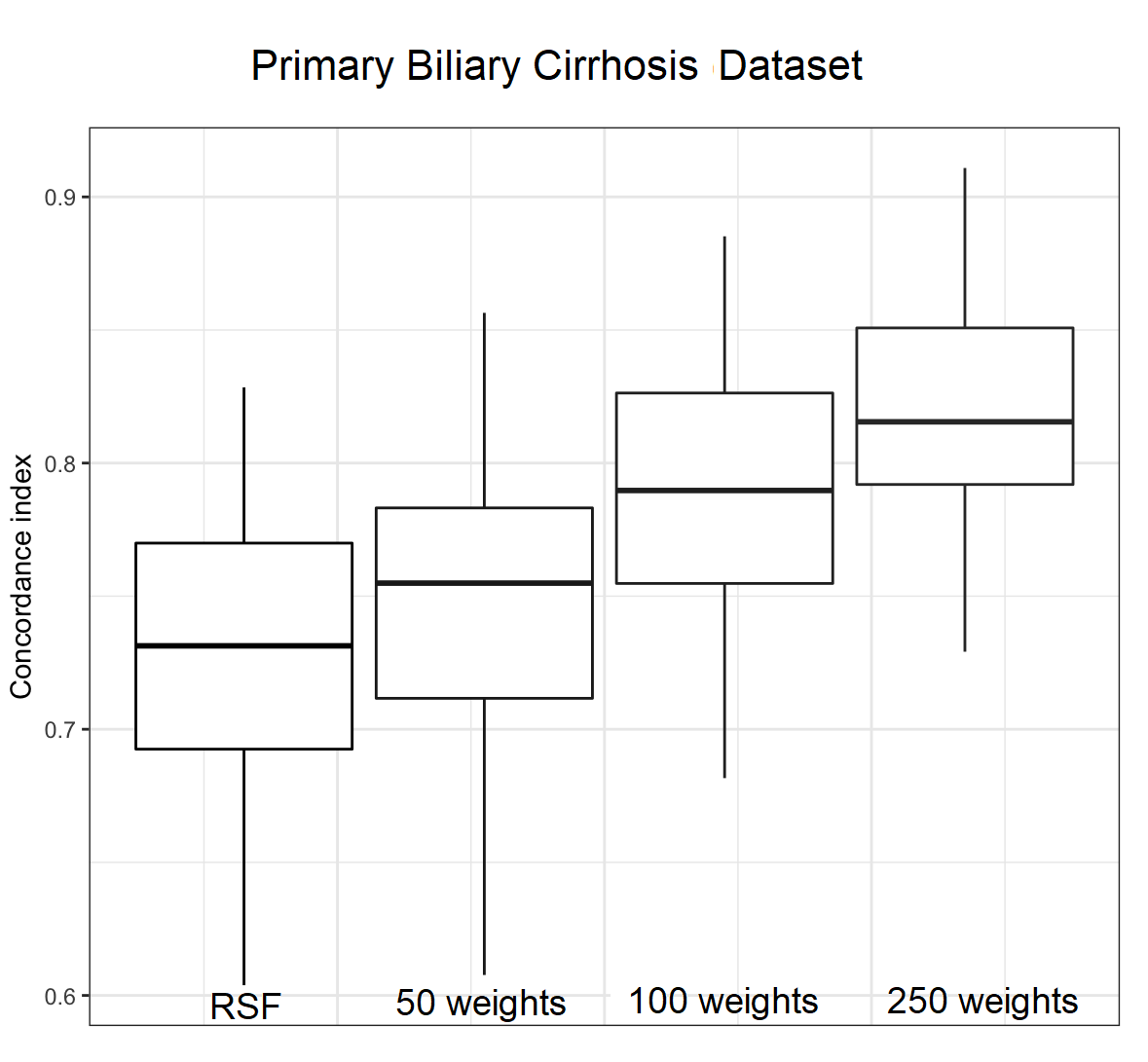
Figure 1: The boxplot for the PBC dataset

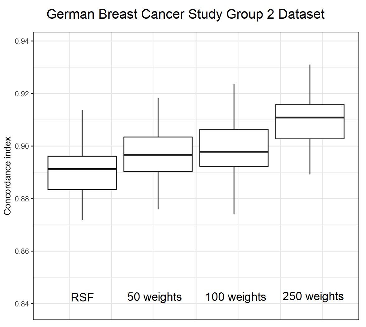
Figure 2: The boxplot for the GCSG2 dataset

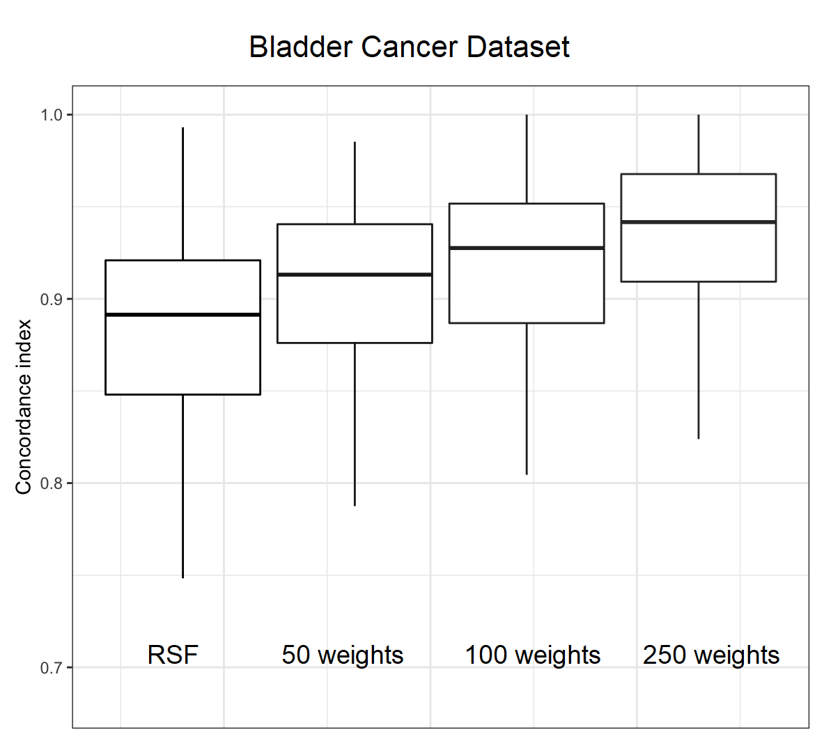
Figure 3: The boxplot for the BLCD dataset

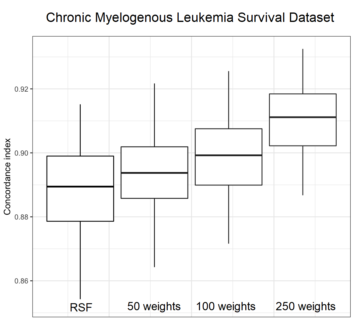
Figure 4: The boxplot for the CML dataset

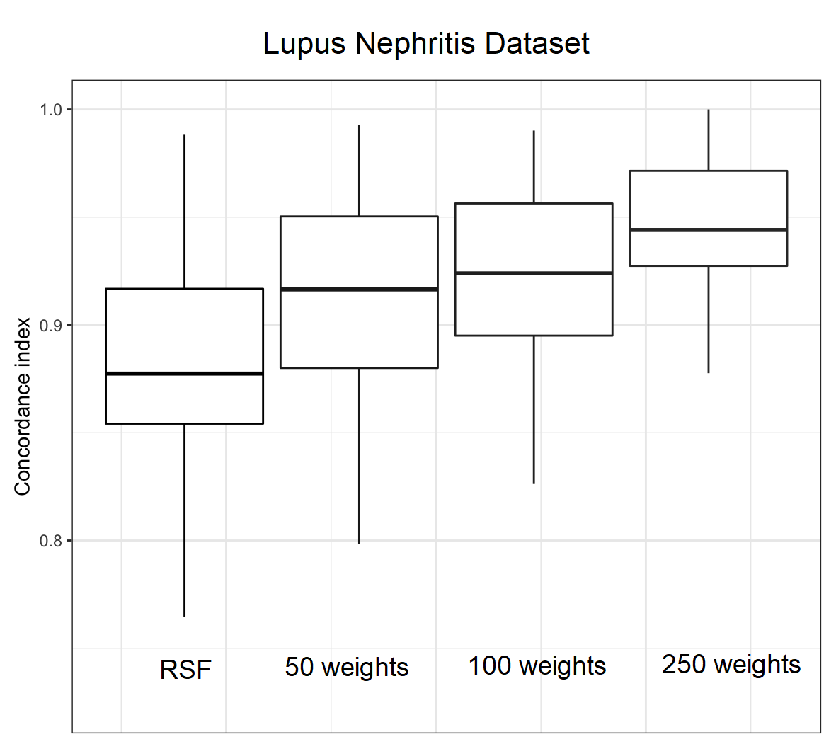
Figure 5: The boxplot for the LND dataset

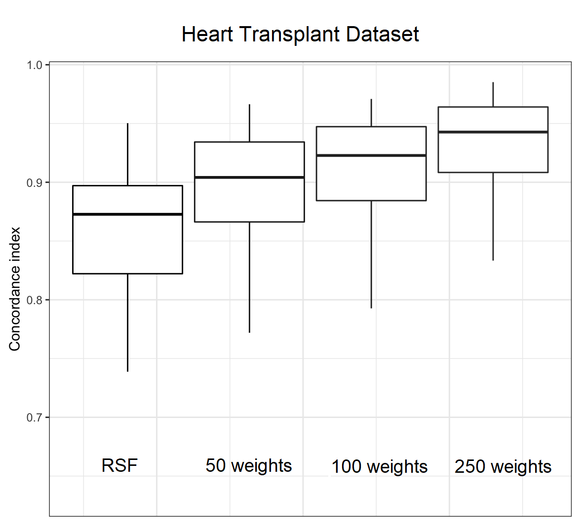
Figure 6: The boxplot for the HTD dataset

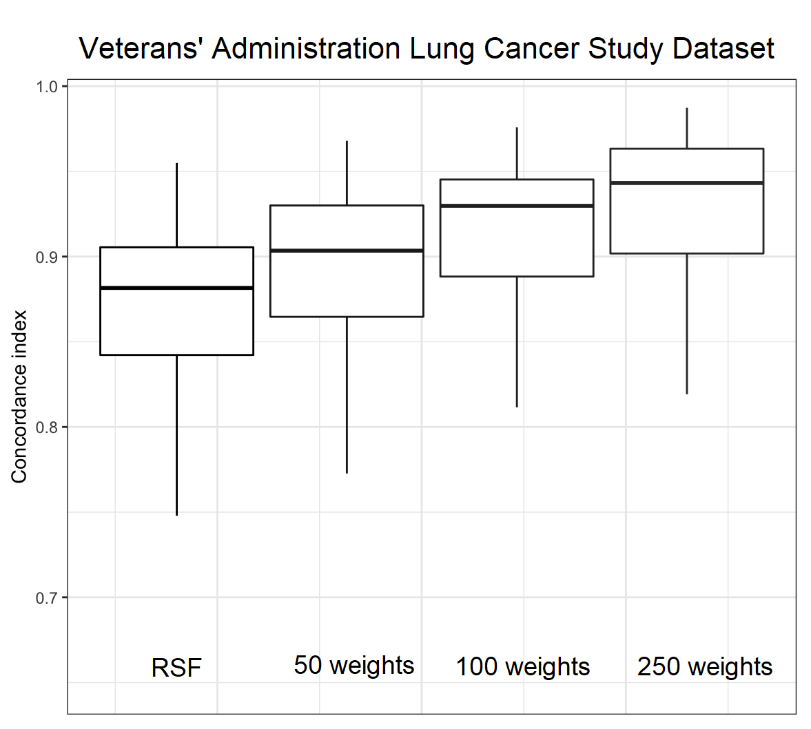
Figure 7: The boxplot for the Veteran dataset

An interesting question is which values of weights are assigned to trees. In order to answer this question, we provide a typical histogram of the weight values derived for the dataset CML (see Fig. 8). The weights are sorted in the descending order. The largest weight is $0.086$, the smallest weight is $4\times 10^{-4}$.

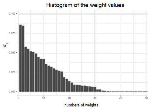
Figure 8: A histogram of the weight values

Another interesting question is how the model performance depends on the number of trees in the random forest. The dependence of the C-index on the number of trees is illustrated in Fig. 9 where the solid and dotted lines correspond to the RSF and the WRSF, respectively. It can be seen from Fig. 9 that the large number of trees may lead even to the performance deterioration when we use the RSF. Whereas the large number of trees improves the WRSF.

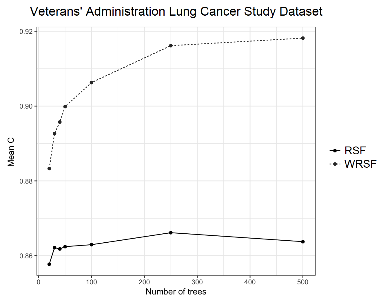
Figure 9: Dependence of the C-index on the number of trees

Our next experiment aims to check whether we can apply the constraint reduction procedure in order to simplify calculations. We reduce the number of constraints by random selection of $K$ constraints for $\xi_{ij}$ from the whole set of constraints which is defined by all pairs of indices in the set $J$. We use again the Veteran dataset for experiments. Fig. 10 shows the dependence of the C-index on the number of selected constraints for optimization. We can see from Fig. 10 that the C-index increases with the number of constraints. Moreover, it is important to note that the C-index for RSF is less than the corresponding C-index for WRSF. This implies that the number of constraints may be reduced in many cases.

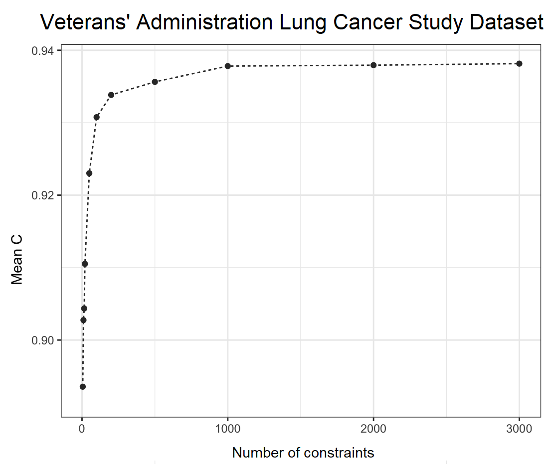
Figure 10: Dependence of the C-index on the number of selected constraints

5 Conclusion

A new survival model based on using the weighted modification of the RSF has been presented in the paper. The main idea underlying this model is to improve the RSF by assigning weights to survival decision trees or to their subsets. The weights are viewed as training parameters. It turns out that this approach provides very improved results especially for some datasets, for example, BLCD, LND, HTD, Veteran. Numerical experiments have illustrated that the proposed model may provide significantly better results in comparison with the original RSF.

The proposed model has several advantages. First, the weights are assigned in accordance with the tree capability to correctly determine the cumulative hazard function. Second, the weights are training parameters which are computed by solving the standard quadratic optimization problem. As a results, the proposed approach is very simple. But the main advantage of the model is that it opens a door for developing a controllable RSF which can solve various machine learning problems in the framework of survival analysis, including, for example, transfer learning. This can be done by changing the loss function which depends on the weights. The consideration of these problems is a direction for further research.

We have studied only the case of linear dependence of the C-index on the weights. However, it is interesting to consider non-linear cases. One of the ways for implementing this case is to use a neural network which is trained to maximize the obtained C-index. The application of the neural network as an additional element of WRSF is also a direction for further research.

Another problem of the WRSF as well as the RSF is that the number of cases when $\mathbf{x}_{i}$ falls into the $k$-th terminal node of a tree may be very small. It makes confidence bounds for the Nelson–Aalen estimator, which estimates the cumulative hazard function, to be very large. The development of robust models taking into account this problem is another direction for further research.

References

- [1] M. Abrahamowicz, T. MacKenzie, and J.M. Esdaile. Time-dependent hazard ratio: modelling and hypothesis testing with application in lupus nephritis. JASA, 91:1432–1439, 1996.
- [2] P. Afshar, A. Mohammadi, K.N. Plataniotis, A. Oikonomou, and H. Benali. From hand-crafted to deep learning-based cancer radiomics: Challenges and opportunities. arXiv:1808.07954v1, Aug 2018.
- [3] H. Akai, K. Yasaka, A. Kunimatsu, M. Nojima, T. Kokudo, N. Kokudo, K. Hasegawa, O. Abe, K. Ohtomo, and S. Kiryu. Predicting prognosis of resected hepatocellular carcinoma by radiomics analysis with random survival forest. Diagnostic and Interventional Imaging, 99(10):643–651, 2018.
- [4] V. Van Belle, K. Pelckmans, S. Van Huffel, and J.A. Suykens. Support vector methods for survival analysis: a comparison between ranking and regression approaches. Artificial intelligence in medicine, 53(2):107–118, 2011.
- [5] V. Van Belle, K. Pelckmans, J.A.K. Suykens, and S. Van Huffel. Support vector machines for survival analysis. In Proceedings of the Third International Conference on Computational Intelligence in Medicine and Healthcare (CIMED2007), pages 1–8, 2007.
- [6] V. Van Belle, K. Pelckmans, J.A.K. Suykens, and S. Van Huffel. Survival svm: a practical scalable algorithm. In ESANN, pages 89–94, 2008.
- [7] G. Biau and E. Scornet. A random forest guided tour. Test, 25(2):197–227, 2016.
- [8] I. Bou-Hamad, D. Larocque, and H. Ben-Ameur. Discrete-time survival trees and forests with time-varying covariates: application to bankruptcy data. Statistical Modelling, 11(5):429–446, 2011.
- [9] I. Bou-Hamad, D. Larocque, and H. Ben-Ameur. A review of survival trees. Statistics Surveys, 5:44–71, 2011.
- [10] L. Breiman. Random forests. Machine learning, 45(1):5–32, 2001.
- [11] A. Ciampi. Generalized regression trees. Computational Statistics & Data Analysis, 12:57–78, 1991.
- [12] D.R. Cox. Regression models and life-tables. Journal of the Royal Statistical Society, Series B (Methodological), 34(2):187–220, 1972.
- [13] M.E.H. Daho, N. Settouti, M.E.A. Lazouni, and M.E.A. Chikh. Weighted vote for trees aggregation in random forest. In 2014 International Conference on Multimedia Computing and Systems (ICMCS), pages 438–443. IEEE, April 2014.
- [14] R.B. Davis and J.R. Anderson. Exponential survival trees. Statistics in Medicine, 8(8):947–961, 1989.
- [15] K. Devarajn and N. Ebrahimi. A semi-parametric generalization of the cox proportional hazards regression model: Inference and applications. Computational Statistics & Data Analysis, 55(1):667–676, 2011.
- [16] J. Fan, Y. Feng, and Y. Wu. Borrowing Strength: Theory Powering Applications – A Festschrift for Lawrence D. Brown, volume 6, chapter High-dimensional variable selection for Cox’s proportional hazards model, pages 70–86. Institute of Mathematical Statistics, 2010.
- [17] D. Faraggi and R. Simon. A neural network model for survival data. Statistics in medicine, 14(1):73–82, 1995.
- [18] T.R. Fleming and D.P. Harrington. Counting processes and survival aalysis. John Wiley & Sons, Hoboken, NJ, USA, 1991.
- [19] J. Gilhodes, C. Zemmour, S. Ajana, A. Martinez, J.-P. Delord, E. Leconte, J.-M. Boher, and T. Filleron. Comparison of variable selection methods for high-dimensional survival data with competing events. Computers in Biology and Medicine, 91:159–167, 2017.
- [20] L. Gordon and R.A. Olshen. Tree-structured survival analysis. Cancer treatment reports, 69(10):1065–1069, 1985.
- [21] C. Haarburger, P. Weitz, O. Rippel, and D. Merhof. Image-based survival analysis for lung cancer patients using cnns. arXiv:1808.09679v1, Aug 2018.
- [22] F. Harrell, R. Califf, D. Pryor, K. Lee, and R. Rosati. Evaluating the yield of medical tests. Journal of the American Medical Association, 247:2543–2546, 1982.
- [23] R. Hehlmann, H. Heimpel, J. Hasford, H.J. Kolb, H. Pralle, D.K. Hossfeld, W. Queisser, H. Loeffler, A. Hochhaus, and B. Heinze. Randomized comparison of interferon-alpha with busulfan and hydroxyurea in chronic myelogenous leukemia. the german cml study group. Blood, 84(12):4064–4077, 1994.
- [24] D. Hosmer, S. Lemeshow, and S. May. Applied Survival Analysis: Regression Modeling of Time to Event Data. John Wiley & Sons, New Jersey, 2008.
- [25] T. Hothorn, P. Bühlmann, S. Dudoit, A. Molinaro, and M.J. van der Laan. Survival ensembles. Biostatistics, 7(3):355–373, 2006.
- [26] C. Hu and J.A. Steingrimsson. Personalized risk prediction in clinical oncology research: Applications and practical issues using survival trees and random forests. Journal of Biopharmaceutical Statistics, 28(2):333–349, 2018.
- [27] X. Huang, S. Chen, and S. Soong. Piecewise exponential survival trees with time-dependent covariates. Biometrics, 54:1420–1433, 1998.
- [28] N.A. Ibrahim, A. Kudus, I. Daud, and M.R. Abu Bakar. Decision tree for competing risks survival probability in breast cancer study. International Journal Of Biological and Medical Research, 3(1):25–29, 2008.
- [29] H. Ishwaran, E.H. Blackstone, C.E. Pothier, and M.S. Lauer. Relative risk forests for exercise heart rate recovery as a predictor of mortality. Journal of the American Statistical Association, 99:591–600, 2004.
- [30] H. Ishwaran and U.B. Kogalur. Random survival forests for r. R News, 7(2):25–31, 2007.
- [31] H. Ishwaran, U.B. Kogalur, E.H. Blackstone, and M.S. Lauer. Random survival forests. Annals of Applied Statistics, 2:841–860, 2008.
- [32] J. Kalbfleisch and R. Prentice. The Statistical Analysis of Failure Time Data. John Wiley and Sons, New York, 1980.
- [33] S. Kaneko, A. Hirakawa, and C. Hamada. Enhancing the lasso approach for developing a survival prediction model based on gene expression data. Computational and Mathematical Methods in Medicine, 2015(Article ID 259474):1–7, 2015.
- [34] J.L. Katzman, U. Shaham, A. Cloninger, J. Bates, T. Jiang, and Y. Kluger. Deepsurv: Personalized treatment recommender system using a Cox proportional hazards deep neural network. BMC medical research methodology, 18(24):1–12, 2018.
- [35] M. Khalilia, S. Chakraborty, and M. Popescu. Predicting disease risks from highly imbalanced data using random forest. BMC Medical Informatics and Decision Making, 11(51):1–13, 2011.
- [36] F.M. Khan and V.B. Zubek. Support vector regression for censored data (svrc): a novel tool for survival analysis. In Proceedings of the IEEE International Conference on Data Mining (ICDM), pages 863–868. IEEE, 2008.
- [37] H. Kim, H. Kim, H. Moon, and H. Ahn. A weight-adjusted voting algorithm for ensemble of classifiers. Journal of the Korean Statistical Society, 40(4):437–449, 2011.
- [38] J. Kim, I. Sohn, S.-H. Jung, S. Kim, and C. Park. Analysis of survival data with group lasso. Communications in Statistics - Simulation and Computation, 41(9):1593–1605, 2012.
- [39] O. Krasotkina and V. Mottl. A bayesian approach to sparse Cox regression in high-dimentional survival analysis. In Proceedings of the 11th International Conference on Machine Learning and Data Mining in Pattern Recognition, volume 9166, pages 425–437, New York, 2015. Springer-Verlag.
- [40] M. LeBlanc and J. Crowley. Relative risk trees for censored survival data. Biometrics, 48(2):411–425, 1992.
- [41] E.T. Lee and J.W. Wang. Statistical Methods for Survival Data Analysis. John Wiley & Sons, New Jersey, 2003.
- [42] H. B. Li, W. Wang, H. W. Ding, and J. Dong. Trees weighting random forest method for classifying high-dimensional noisy data. In 2010 IEEE 7th International Conference on E-Business Engineering, pages 160–163. IEEE, Nov 2010.
- [43] A. Linden and P.R. Yarnold. Modeling time–to–event (survival) data using classification tree analysis. Journal of Evaluation in Clinical Practice, 23(6):1299–1308, 2017.
- [44] M. Luck, T. Sylvain, H. Cardinal, A. Lodi, and Y. Bengio. Deep learning for patient-specific kidney graft survival analysis. arXiv:1705.10245, May 2017.
- [45] M. May, P. Royston, M. Egger, A.C. Justice, and J.A.C. Sterne. Development and validation of a prognostic model for survival time data: application to prognosis of HIV positive patients treated with antiretroviral therapy. Statistics in Medicine, 23:2375–2398, 2004.
- [46] F. Miao, Y.-P. Cai, Y.-X. Zhang, Y. Li, and Y.-T. Zhang. Risk prediction of one-year mortality in patients with cardiac arrhythmias using random survival fores. Computational and mathematical methods in medicin, 2015:1–10, 2015. Article ID 303250.
- [47] U.B. Mogensen, H. Ishwaran, and T.A. Gerds. Evaluating random forests for survival analysis using prediction error curves. Journal of Statistical Software, 50(11):1–23, 2012.
- [48] J.B. Nasejje, H. Mwambi, K. Dheda, and M. Lesosky. A comparison of the conditional inference survival forest model to random survival forests based on a simulation study as well as on two applications with time-to-event data. BMC Medical Research Methodology, 17(115):1–17, 2017.
- [49] M.Z. Nezhad, N. Sadati, K. Yang, and D. Zhu. A deep active survival analysis approach for precision treatment recommendations: Application of prostate cancer. arXiv:1804.03280v1, April 2018.
- [50] I.K. Omurlu, M. Ture, and F. Tokatli. The comparisons of random survival forests and cox regression analysis with simulation and an application related to breast cancer. Expert Systems with Applications, 36:8582–8588, 2009.
- [51] M. Pagano and K. Gauvreau. Principles of biostatistics. Pacific Grove, CA : Duxbury, 2000.
- [52] S. Polsterl, N. Navab, and A. Katouzian. An efficient training algorithm for kernel survival support vector machines. arXiv:1611.07054v, Nov 2016.
- [53] R. Ranganath, A. Perotte, N. Elhadad, and D. Blei. Deep survival analysis. arXiv:1608.02158, September 2016.
- [54] C.A. Ronao and S.-B. Cho. Random forests with weighted voting for anomalous query access detection in relational databases. In Artificial Intelligence and Soft Computing. ICAISC 2015, volume 9120 of Lecture Notes in Computer Science, pages 36–48, Cham, 2015. Springer.
- [55] W. Sauerbrei and P. Royston. Building multivariable prognostic and diagnostic models: transformation of the predictors by using fractional polynomials. Journal of the Royal Statistics Society Series A, 162(1):71–94, 1999.
- [56] M. Schmid, M.N. Wright, and A. Ziegler. On the use of harrell’s c for clinical risk prediction via random survival forests. Expert Systems with Applications, 63:450–459, 2016.
- [57] B. Scholkopf and A.J. Smola. Learning with Kernels: Support Vector Machines, Regularization, Optimization, and Beyond. The MIT Press, Cambridge, Massachusetts, 2002.
- [58] M.R. Segal. Regression trees for censored data. Biometrics, 44(1):35–47, 1988.
- [59] P.K. Shivaswamy, W. Chu, and M. Jansche. A support vector approach to censored targets. In Seventh IEEE International Conference on Data Mining, ICDM 2007, pages 655–660. IEEE, 2007.
- [60] X.G. Su and J.J. Fan. Multivariate survival trees: a maximum likelihood approach based on frailty models. Biometrics, 60(1):93–99, 2004.
- [61] J.M.G. Taylor. Random survival forests. Journal of Thoracic Oncology, 6(12):1974–1975, 2011.
- [62] N. Ternes, F. Rotolo, and S. Michiels. Empirical extensions of the lasso penalty to reduce the false discovery rate in high-dimensional cox regression models. Statistics in medicine, 35(15):2561–2573, 2016.
- [63] R. Tibshirani. The lasso method for variable selection in the cox model. Statistics in medicine, 16(4):385–395, 1997.
- [64] H. Wang and L. Zhou. Random survival forest with space extensions for censored data. Artificial intelligence in medicine, 79:52–61, 2017.
- [65] P. Wang, Y. Li, and C.K. Reddy. Machine learning for survival analysis: A survey. arXiv:1708.04649, August 2017.
- [66] A. Widodo and B.-S. Yang. Machine health prognostics using survival probability and support vector machine. Expert Systems with Applications, 38(7):8430–8437, 2011.
- [67] D.M. Witten and R. Tibshirani. Survival analysis with high-dimensional covariates. Statistical Methods in Medical Research, 19(1):29–51, 2010.
- [68] M.N. Wright, T. Dankowski, and A. Ziegler. Random forests for survival analysis using maximally selected rank statistics. arXiv:1605.03391v1, May 2016.
- [69] M.N. Wright, T. Dankowski, and A. Ziegler. Unbiased split variable selection for random survival forests using maximally selected rank statistics. Statistics in Medicine, 36(8):1272–1284, 2017.
- [70] L. Wrobel, A. Gudys, and M. Sikora. Learning rule sets from survival data. BMC Bioinformatics, 18(1):285–297, 2017.
- [71] J. Yao, X. Zhu, F. Zhu, and J. Huang. Deep correlational learning for survival prediction from multi-modality data. In Medical Image Computing and Computer–Assisted Intervention – MICCAI 2017, volume 10434 of Lecture Notes in Computer Science, pages 406–414. Springer, Cham, 2017.
- [72] J. Yoon, W.R. Zame, A. Banerjee, M. Cadeiras, A.M. Alaa, and M. van der Schaar. Personalized survival predictions via trees of predictors: An application to cardiac transplantation. PLoS ONE, 13(3:e0194985):1–19, 2018.
- [73] H. Zhang. Splitting criteria in survival trees. In 10th Workshop on Statistical Modelling, volume Lecture notes in statistical series, pages 305–314, New York, 1995. Springer.
- [74] H.H. Zhang and W. Lu. Adaptive Lasso for Cox’s proportional hazards model. Biometrika, 94(3):691–703, 2007.
- [75] X. Zhu, J. Yao, and J. Huang. Deep convolutional neural network for survival analysis with pathological images. In 2016 IEEE International Conference on Bioinformatics and Biomedicine (BIBM), pages 544–547. IEEE, 2016.