The CARMA-NRO Orion Survey

Abstract

Context. We present an initial overview of the filamentary structure in the Orion A molecular cloud utilizing a high angular and velocity resolution C¹⁸O(1–0) emission map that was recently produced as part of the CARMA-NRO Orion Survey.

Aims. The main goal of this study is to build a credible method to study varying widths of filaments which has previously been linked to star formation in molecular clouds. Due to the diverse star forming activities taking place throughout its $\sim$20 pc length, together with its proximity of 388 pc, the Orion A molecular cloud provides an excellent laboratory for such an experiment to be carried out with high resolution and high sensitivity.

Methods. Using the widely-known structure identification algorithm, DisPerSE, on a 3-dimensional (PPV) C¹⁸O cube, we identified 625 relatively short (the longest being 1.74 pc) filaments over the entire cloud. We study the distribution of filament widths using FilChaP, a python package that we have developed and made publicly available.

Results. We find that the filaments identified in a 2 square degree PPV cube do not overlap spatially, except for the complex OMC-4 region that shows distinct velocity components along the line of sight. The filament widths vary between 0.02 and 0.3 pc depending on the amount of substructure that a filament possesses. The more substructure a filament has, the larger is its width. We also find that despite this variation, the filament width shows no anticorrelation with the central column density which is in agreement with previous Herschel observations.

1 Introduction

Over the past decade, it has become clear that stars preferentially form along and at the junctions of filaments inside cold, dense molecular clouds (e.g. Schneider et al. 2012). Filaments pervade molecular clouds whether these clouds form high-mass or low-mass stars, or lack star formation entirely (André et al. 2010, 2016). Earlier studies of dust continuum observed with the Herschel Space Observatory suggest a “universal width” of the observed filaments (Arzoumanian et al. 2011). The distribution of widths of 90 filaments having column densities of 10²⁰ – 10²³ cm^-2 peaks at 0.1 pc with very little dispersion ($\pm$0.03 pc, Arzoumanian et al. 2011). However, work by Smith et al. (2014) shows that the calculated filament width is dependent on the fitting range considered when analyzing the radial profiles. They found that the degeneracy between the central density of the filaments and their inner flat-radius raises uncertainties. We also refer to Panopoulou et al. (2017) for the shortcomings of fitting methods used in calculating filament widths. Moreover, higher angular resolution observations that allow study of high density filaments within molecular clouds suggest widths as narrow as 0.01 pc (Sánchez-Monge et al. 2014; Hacar et al. 2018), while observations of tracers such as ¹³CO have revealed filaments with 0.4 pc widths (Panopoulou et al. 2014a). For the study of filament properties, in particular their widths, molecular line observations allow studying intertwined filamentary networks which otherwise appear as single objects when observed in dust emission due to projection of 3-dimensional information (position-position-velocity, hereafter; PPV) on to 2-dimensional column density space, therefore providing a more accurate determination of the filament properties. Understanding the role of filaments in the process of star formation requires high spatial and spectral resolution studies of, ideally, multiple molecular emission lines that trace different densities within the cloud, as well as continuum emission. This way, filament properties can be calculated for different tracers that probe a variety of physical and chemical conditions. Investigating physical and kinematic properties of filaments weighted by the environmental and chemical conditions allows us to gain an understanding of how filaments form, how this relates to the formation of molecular clouds, how mass flow and/or accretion onto filaments leads to the formation of new stars (see e.g. Ostriker 1964; Larson 1985; Inutsuka & Miyama 1992; Pon et al. 2012; Fischera & Martin 2012; Heitsch 2013; Smith et al. 2014; Clarke & Whitworth 2015; Seifried & Walch 2015; Clarke et al. 2016; Smith et al. 2016; Clarke et al. 2017; Chira et al. 2018).

In this work, we study filament properties towards the closest site of ongoing high-mass star formation, the Orion A molecular cloud ($d\approx 388$ pc, Kounkel et al. 2017). Orion A is amongst the most studied regions in the Galaxy (e.g. Bally et al. 1987; Johnstone & Bally 1999; Shimajiri et al. 2009; Nakamura et al. 2012). The northern Orion A region, encompassing OMC-1, OMC-2, OMC-3 and OMC-4, is commonly referred as the Integral Shaped Filament (hereafter; ISF, Bally et al. 1987). The whole ISF is subject to ionizing UV radiation produced by the Trapezium stars $\sim 1$ pc in front of the molecular cloud (van der Werf et al. 2013). Moreover, the NGC1977 HII region, powered by a B0V type star, 42 Ori, could produce a radiation field as strong as 2000 times the standard value of the ISRF (G₀ $\simeq$ 2000) on the OMC-3 filaments, depending on the 3D orientation of the star relative to the northern ISF. Towards the south, the ISF extends to the L1641 region that is more diffuse compared to the northern portion, and less affected by the UV radiation due to the lack of high-mass stars.The structures seen in Orion A are therefore shaped not only by the gravitational potential of OMC-1, but also by the feedback from high-mass and low-mass (proto)stars.

So far, large-scale spectral line emission maps of the Orion A cloud have been obtained only with low angular resolution, while high angular resolution observations have been obtained only towards selected sub-regions of the cloud. For example, while Bally et al. (1987) observed a 1.5 square degree region of the ISF with a 0.1 pc resolution, Kainulainen et al. (2017) has observed a 3 x 11 arcmin (0.33 x 1.24 pc) region towards OMC-2 with a $\sim$1200 AU resolution. Similarly, Hacar et al. (2018) observed a narrow field around the OMC-1/OMC-2 regions with high angular resolution (1750 AU) using a map combining data from ALMA and the IRAM 30m telescope. The current work, on the other hand, provides a first look into filament properties that are obtained with high angular resolution in an extensive map of the Orion A molecular cloud.

In Section 2, we summarize the large scale and high angular resolution observations from the CARMA-NRO Orion Survey. In Section 3 we introduce our methods to calculate physical properties of filaments. Based on these methods we present filament properties as observed in C¹⁸O emission, see Section 4. Finally, we summarize our results in Section 5.

2 Observations

In order to image an extended region towards Orion A with high angular resolution and high sensitivity, the CARMA-NRO Orion Survey (PI: J. Carpenter) was granted $\sim$650 hours of observing time at the Combined Array for Millimeter-Wave Astronomy (CARMA). The observations were carried out between 2013 and 2015 using 15 antennas (6 and 10 m dishes) of the array with D and E configurations resulting in an angular resolution of about 8 arcsec (0.015 pc at a distance of 388 pc). Outflow and diffuse gas tracers (¹²CO and ¹³CO), warm dense gas tracers (CS and C¹⁸O), a cold dense gas tracer (CN) and a shock tracer (SO) along with the 3 mm continuum were observed simultaneously. The interferometric observations were combined with single dish observations in order to account for extended emission. The single dish observations were carried out at the 45 m telescope at the Nobeyama Radio Observatory (NRO45m). The NRO45m data were taken using two different receivers; BEARS between 2007 and 2009 for ¹²CO, and between 2013 and 2014 for ¹³CO and C¹⁸O, and FOREST between 2014 and 2017. These observations are described in detail in Shimajiri et al. (2014) and Kong et al. (2018), respectively. For combination and joint deconvolution of the interferometer and single dish data in the uv-domain the method presented by Koda et al. (2011) was followed. The data combination results in 0.47 K rms noise level in 0.22 km s^-1 channels. Details on the imaging are presented in the CARMA-NRO Orion Survey data paper Kong et al. (2018).

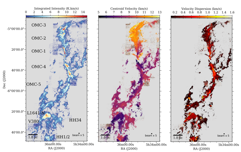
The combined (CARMA+NRO45m) data spans 2 degrees in declination including the ISF in the north and the L1641 cloud in the south. In Figure 1, we show the C¹⁸O moment maps; integrated intensity, centroid velocity and velocity dispersion (from left to right). The data highlights the filamentary nature of the cloud (see Figure 1, left panel), as well as hub-like structures where filaments merge. A plethora of kinematic information accompanying the filamentary structure can be seen in the velocity centroid map (Figure 1, middle panel). In addition to the well known north-south velocity gradient from 13 km s^-1to 5 km s^-1, we see gradients perpendicular to the spine of the ISF appearing in OMC-4 and -5 regions. The kinematics of the filamentary structure will be discussed in a following paper.

Figure 1: Moment maps of C¹⁸O J = 1–0. From left to right the panels display the integrated intensity emission, the centroid velocity, and the velocity dispersion. Relevant star-forming regions are marked on the integrated intensity map. Beam-size shown in the bottom left corner is five times the real beam-size (5x0.015 pc) of the observations for demonstration purposes.

3 Filament properties

Filament identification is done by employing the structure identification algorithm Discrete Persistent Structures Extractor, DisPerSE (Sousbie 2011). DisPerSE uses the Morse theory to derive information on the topology of a given data set. It builds up a tessellation consisting of critical points – those points where the gradient of the intensity goes to zero, namely: minima, maxima and saddle points. It connects maxima and saddle points via arcs, which are then called filaments. DisPerSE has been a widely used tool to extract filamentary structures both in observational and synthetic datasets (e.g. Arzoumanian et al. 2011; Schneider et al. 2012; Palmeirim et al. 2013; Panopoulou et al. 2014b; Smith et al. 2016; Chira et al. 2018). In order to identify filaments in the CARMA-NRO Orion Survey we use the C¹⁸O datacube. The C¹⁸O emission allows us to trace denser regions of the cloud. It is optically thin and less affected by stellar feedback compared to ¹²CO and ¹³CO, therefore it is a better choice to trace dense filaments. The ¹²CO emission traces more diffuse and optically thick parts of the cloud (see Figure 5 in Kong et al. 2018), and therefore we refrain from using it for the analysis of the filamentary structure. The ¹³CO map shows filamentary structure in addition to the extended emission (see Figure 6 in Kong et al. 2018), but it can be optically thick in the densest parts of the ISF.

We apply DisPerSE on the C¹⁸O datacube with a persistence and a noise threshold of 2 K (4 $\sigma$). Persistence is a term that refers to the contrast between the values of the identified critical points. High persistence means that the identified maximum has higher contrast with respect to its surroundings. Eliminating those critical point pairs with low persistence, in turn, leaves us with the most prominent structures that stand out from the rest. For further discussion on persistence and the general mathematical background of the algorithm we refer to Sousbie (2011).

After running on a 3-dimensional position-position-velocity (PPV) cube, DisPerSE provides us with filament coordinates for each identified filament on the PPV space. This has an advantage over the column density filaments identified in Herschel maps (e.g. André et al. 2016), because we are able to disentangle the velocity structure of the filaments instead of looking at integrated emission over all the structure along the line of sight.

Figure 2: Filaments identified in the Orion A molecular cloud. Greyscale shows the C¹⁸O peak intensity emission, while the colored segments indicate the filaments identified by DisPerSE.

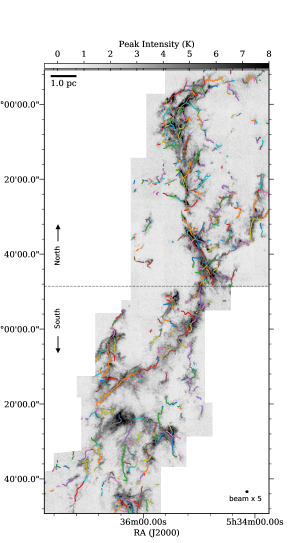
Figure 2 shows the identified filaments overlaid on the C¹⁸O peak intensity map. In total, 347 filaments are identified in the northern region (ISF) and 278 filaments in the southern region (northern part of the L1641 cloud). The properties of these filaments are unaffected by the recent distance measurements to the cloud that showed a distance gradient throughout Orion A (Grossschedl et al. 2018). The gradient starts being effective below galactic longitude 210^∘ (or approximately $-$6^∘30^′) close to the southern border of our map. The filaments show slightly different properties in the northern part of the cloud compared to the more diffuse filaments identified in the southern part (see the following sections and Figures 5 and 10). A large number of filaments identified by DisPerSE have short lengths (¡ 0.15 pc), and seem to be continuations of one another, resulting in a longer but fragmented (as seen in C¹⁸O) filament. We therefore do not exclude them from further analysis, in particular for the width determination. However, properties of only those filaments with an aspect ratio larger than 2:1 are shown in the Appendix B.

In order to study filament properties, we have developed a python package: the Filament Characterization Package FilChaP that utilizes the coordinates of the identified filaments and derives their physical properties. In the following section, we present the analysis performed by FilChaP.

3.1 Calculation of the filament width

For each filament, we extract radial intensity profiles perpendicular to the filament spines. This is done by first calculating coordinates of a perpendicular line at each sample point along each spine. These sample points are separated by 1.5 beam sizes (0.023 pc) in order to provide statistical independence. This separation value was found by visual inspection of the pixels employed to produce intensity profiles, making sure the same pixels are not used multiple times in consecutive slices. However, depending on a filament’s curvature, the slices may occasionally cross one another at larger radial distances from the spines. The pixels that lie on or adjacent to the calculated perpendicular lines are used to produce the radial intensity profiles in a similar fashion to Duarte-Cabral & Dobbs (2016).

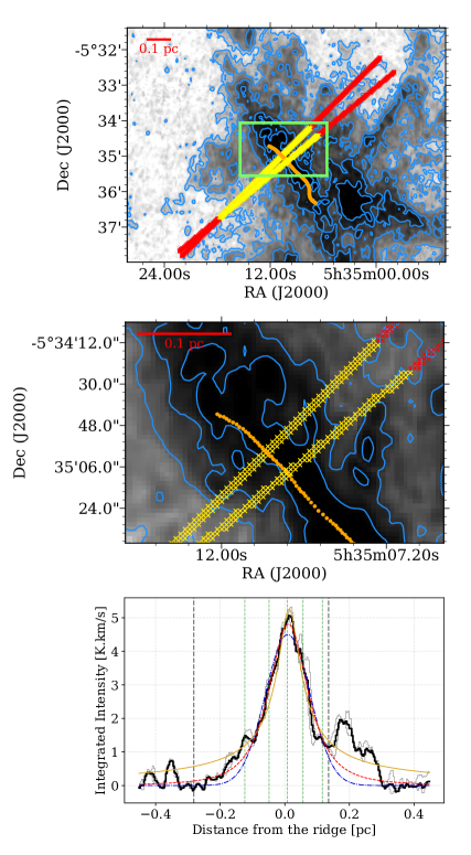
This process is shown in Figure 3. On the top panel of the figure the peak intensity map towards the OMC-4 region that is overlaid with an identified filament spine is shown. Two perpendicular slices from which we extract intensity profiles are also overlaid on the filament spine in red. An intensity profile is constructed using intensities of the pixels that are perpendicular to the filament spine at a sample spine point. These “perpendicular pixels” are found on or at the immediate vicinity of the calculated perpendicular line by looking for pixels that are at most 1 pixel away from the perpendicular line. The middle panel of Figure 3 shows an expanded view of the region marked with a green box in the rop panel, in order to provide a more detailed look into the perpendicular slices. The perpendicular pixels are shown with red crosses marking the center of each pixel. There are occurrences where the calculated perpendicular lines do not cross exactly pixel centers. In that case, FilChaP takes the mean of the intensities from pixels that lie adjacent to the perpendicular lines. A complete radial intensity profile is achieved by plotting intensities from perpendicular pixels at each radial distance from the filament spine.

The bottom panel of Figure 3 shows the averaged (over the shown two perpendicular slices) and baseline subtracted intensity profile with a black solid line. In order to obtain the averaged profiles, we take the mean of the intensities at each radial distance from the spine. The negative distances from the spine point to the north-east direction, and positive distances to south-west of the filament. The grey thin lines indicate the different profiles extracted from each slice. Blue, yellow and red curves fitted to the averaged intensity profiles in the right panel denote Gaussian and Plummer–like fits with p=2 and 4, respectively. Grey dashed lines indicate the fitting boundaries. Green dashed lines indicate the shoulders of the averaged profile. A shoulder is identified where there is a local minimum in the second derivative of an intensity profile. Within FilChaP the shoulders are always identified on the smoothed intensity profiles. For this study, the smoothing length is the beam size. We also require the integrated intensity of a shoulder to be at least five times the noise level of the averaged profile which on the order of 1 K. km s^-1. This threshold is set in order to discard less significant peaks.

Figure 3: Top: C¹⁸O peak intensity emission overlaid with a filament spine (in orange) and 2 perpendicular slices (in red and yellow). The yellow portion of the slices indicate the extent of emission fitted with FilChaP. The green box marks the zoom-in region shown in the middle panel. Contours indicate emission levels of 2, 3, 5, 7, 9, 11 K. Middle: Expanded view of the perpendicular slices. The perpendicular pixels used to extract the intensities at each radial bin are marked with crosses. Bottom: The intensity profiles (grey lines) extracted from the slices overlaid on the map in the middle panel. Blue, yellow and red curves fitted to the averaged intensity profile (black) indicate Gaussian and Plummer-like fits with p=2 and 4, respectively. The vertical grey dashed lines show the positions of the identified minima considered during the fitting procedure (see Sect. 3.1). Vertical green dashed lines correspond to shoulders as explained in Sect. 4.1.

As each point on the identified filament is defined by a velocity coordinate as well, we know the velocity range spanned by our filament. This information allows us to disentangle filamentary structure in PPV space. Therefore, we utilize this information when calculating the radial intensity profiles in the following way. The intensity profiles are not calculated on the integrated intensity map that is obtained from the entire velocity range of the cloud (as was done in the dust continuum studies). Instead, the intensities from each perpendicular slice are integrated over the two neighbouring velocity channels around the velocity at which the filament is identified. For example, if a point along the filament is at a velocity of 5.5 km s^-1 the intensity profile that is perpendicular to this point is calculated from the integrated intensity between 5.28 km s^-1 and 5.72 km s^-1 with the velocity channel width being 0.22 km s^-1. This helps reduce the confusion in PPV space by discarding emission other than that which belongs to the identified filament and it makes sure that the emission included in the construction of the intensity profiles is not separated from the velocity at which the filament is identified by more than 2 times the sound speed (approximately 0.2 km s^-1 at 10 K , close to our velocity resolution), providing coherence. The velocity coordinate along the filaments often change, therefore, the integrated intensities are computed individually for each PPV point along a filament.

3.1.1 Filament width determination methods

In order to calculate the widths, we employ four different methods, a Gaussian fit, two fits with Plummer–like functions with power law indices p=2 and 4, and the second moment of distribution. Plummer-like functions have been used to describe the column density of a filament with a dense and flat inner portion and a power-law decline at larger radii (Arzoumanian et al. 2011):

$$\Sigma_{p}(r)=A_{p}\frac{\rho_{c}R_{flat}}{\left[1+\left(\frac{r}{R_{flat}}\right)^{2}\right]^{\left(\frac{p-1}{2}\right)}}$$ (1)

where $\rho_{c}$ is the central density, $R_{flat}$ is the radius within which the density is uniform, $p$ is the power law index, and $A_{p}$ is a finite constant that is related to the filament’s inclination compared to the plane of the sky (here we assume that this angle is zero). The $n^{th}$ moment of a distribution $I$ is given by:

$$m_{n}=\frac{1}{N}\frac{\sum_{i}^{N}I_{i}\left(x_{i}-\bar{x}\right)^{n}}{\sigma^{n}}$$ (2)

where $\bar{x}$ is the intensity weighted mean position of the profile, ${I_{i}}$ is the intensity at position $x_{i}$, and $\sigma$ is the intensity weighted standard deviation of the profile. The second moment is the variance of the distribution and therefore we calculate the width of the profile as $\sqrt{m_{2}}\times 2\sqrt{2ln2}$. For the fits, we use the curve_fit function contained within the scipy.optimize package with the default Levenberg–Marquardt algorithm.

We refrain from fitting the power law index of the Plummer-like function due to the degeneracy between $p$ and $R_{flat}$. Instead, we use the literature values of the index; p=4 for the density of a homogeneous isothermal cylinder (Ostriker 1964) and p=2, the value derived in Herschel studies when p is fitted as a free parameter (Arzoumanian et al. 2011), which is attributed to non-isothermality of these objects (e.g., Lada et al. 1999) or to magnetic fields (e.g., Fiege & Pudritz 2000).

The profiles are fitted only within the boundaries set by the minima around the peak. These boundaries are shown in the right hand side of Figure 3 as grey vertical dashed lines. The minima are automatically calculated through FilChaP by first smoothing the profiles with a Gaussian having a width of the beam-size of the observations, and then looking at minima around the peak with a significance of $\sim$ 3 beam-sizes. If multiple minima are detected on each side of the spine we take the ones that are located closer to the maxima as boundaries. The effect of the fitting range on the calculated widths is further discussed in Section 3.2.2.

3.1.2 Treating the bias caused by the averaging length

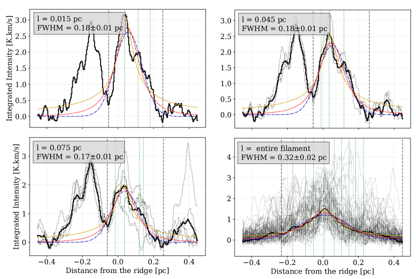
Previous studies (e.g. Arzoumanian et al. 2011) calculated filament widths using intensity profiles that are averaged over the entire length of a filament. Although averaging helps to obtain a smooth radial intensity profile, it has the disadvantage that any information that could be used to understand how and why the width changes along a single filament is lost. Therefore, we first study the effect of averaging intensity profiles by averaging over a length of 0.015 pc (a beam-size), 0.045 pc, 0.075 pc and finally over the entire filament. Figure 4 shows how averaging intensity profiles over different length scales affects the results. The length scale over which the profiles are averaged is indicated on the top left corner of each panel. The panels where we average over shorter length scales (top left and right, bottom left) show marginal change in width. The bottom right panel, however, reveals if we were to average over the length of the filament, the resulting width is twice as large as the previous values. Thus, not only do we overestimate the filament width by averaging, but we also lose information on the sub-structure of the filament. We then choose to average intensity profiles over a length of 0.045 pc (3 beam-sizes) for further analysis. While this approach gives us a chance to smooth the profiles over 12 points (3 beam-sizes) along the filament, it helps us avoid deriving overestimated parameters. Furthermore, we are able to follow the gradient of the width along the identified filaments.

Figure 4: Plots showing the effect of averaging intensity profiles along different length scales. Individual intensity profiles are shown in grey, while averaged intensity profiles are shown in black. Blue, yellow and red curves fitted to the averaged intensity profile (black) indicate Gaussian and Plummer-like fits with p=2 and 4, respectively. The grey vertical dashed lines indicate the fitting boundaries and the green vertical dashed lines indicate the shoulders identified by FilChaP. From the top left to bottom right the profiles are averaged over 0.015, 0.045, 0.075 pc and the entire filament with corresponding Gaussian FWHM of 0.18, 0.18, 0.17 and 0.32 pc.

Figure 5: Distribution of filament widths in the norther (colored) and southern (grey) regions of Orion A (see Fig. 2) calculated using Gaussian fits (top left), the second moment of distribution (bottom right), and Plummer-like fits with power law indices p=2 (top right) and p=4 (bottom left). The vertical dashed lines represent the filament widths from Hacar et al. (2018) in red, and the “characteristic” filament width (Arzoumanian et al. 2011) in black. The dot-dashed line indicates the beam-size of our observations.

3.2 Distribution of filament widths

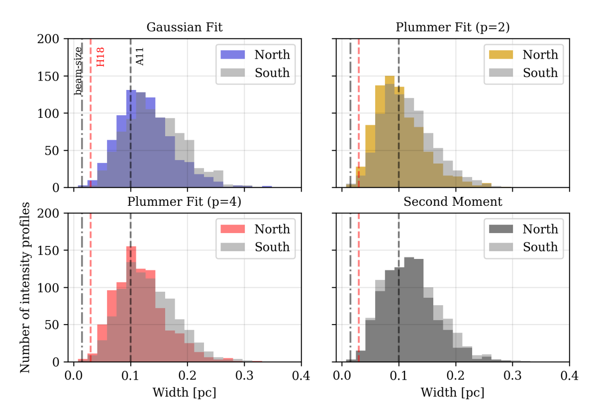
Using the method described in Section 3.1, we calculate the widths of all the 625 filaments identified by DisPerSE in Orion A. The results are shown in Figure 5 where the distribution for the northern region is shown by the colored and the southern region by the grey histograms. The four subplots show the distribution of widths (FWHM) calculated using Gaussian (left) and Plummer p=2 fits (right) in the top panel, Plummer p=4 fit (left) and the FWHM calculated from the second moment of distribution (right) in the bottom panel. Black and red dashed lines in each subplot plot indicates the “characteristic” widths found by Arzoumanian et al. (2011) in Herschel dust continuum, and Hacar et al. (2018) in N₂H⁺ emission. The dot-dashed line indicates the spatial resolution of the data.

All four methods yield similar distributions, with the Plummer p=2 fits resulting in slightly narrower widths. The median values of the distributions are $0.12\begin{subarray}{c}+0.15\\ -0.09\end{subarray}$ pc and $0.14\begin{subarray}{c}+0.18\\ -0.11\end{subarray}$  pc for the Gaussian fits, $0.09\begin{subarray}{c}+0.13\\ -0.07\end{subarray}$  pc and $0.11\begin{subarray}{c}+0.14\\ -0.08\end{subarray}$  pc for the Plummer p=2 fits, $0.11\begin{subarray}{c}+0.14\\ -0.08\end{subarray}$  pc and $0.13\begin{subarray}{c}+0.16\\ -0.09\end{subarray}$  pc for the Plummer p=4 fits, and finally, $0.12\begin{subarray}{c}+0.15\\ -0.09\end{subarray}$  pc and $0.12\begin{subarray}{c}+0.15\\ -0.09\end{subarray}$  pc for the FWHM derived from the second moment for the northern and southern regions, respectively. These results are very close to what has been reported by the Herschel studies (e.g. Arzoumanian et al. 2011; André 2017) and are larger than the width reported based on ALMA studies of filaments (e.g. Hacar et al. 2018; Henshaw et al. 2017), which is not unexpected considering that N₂H⁺ is less extended and traces higher densities along filament spines.

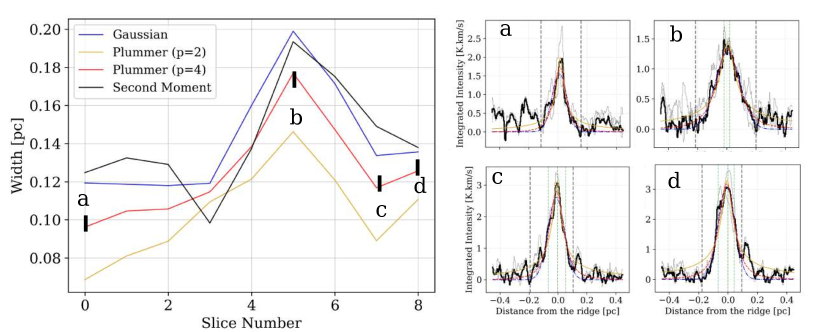
The existence of a “characteristic” filament width is still highly debated (see Panopoulou et al. 2017; André 2017). In studies such as Arzoumanian et al. (2011); Palmeirim et al. (2013); Koch & Rosolowsky (2015) the spread of the filament width distribution is less than a factor of two around the median width. On the other hand, a study by Juvela et al. (2012) shows that there is an order of magnitude deviation from the mean width (0.1–1.0 pc). Our distributions shown in Figure 5 indicate a very significant, about an order of magnitude spread around the median value regardless of the method. The origin of this wide distribution may be due to the fact that the filaments are not isolated homogeneous cylinders. They may have variations along their length that are not taken into account if the entire filament is represented by an averaged number. In Figure 6 we show an example of how the width changes along a single filament. In the left panel, we plot the slice number along the filament (cross-sections for radial intensity profiles) against the calculated width at the corresponding slice. The Plummer p=2 fit yields narrower widths along the filament, this agrees with the general picture that we have drawn from Figure 5. The right panel shows 4 subplots corresponding to 4 intensity profiles along the filament that are marked by “a”, “b”, “c” and “d” in the left panel. These intensity profiles are selected to be representative of how the width changes. At point “a”, the intensity profile is the narrowest and peaky with a width of 0.12 pc (Gaussian FWHM). As we progress from point “a” to “b” we see that the substructures (apparent at around 1 K. km s${}^{-1}\leavevmode\nobreak\$, close to five times the noise level of the averaged profile) that appear at point “a” get wider, hence the width increases. At point “b” the intensity profile is broad and the width is the largest, reaching 0.2 pc. From point “c” to “d” the shoulders on both sides of the peak (shown in green dashed lines) get wider and acquire higher intensities, which in turn causes the increase in width. The unresolved inhomogeneities within the filament itself that can be traced by these shoulders in the profile cause the filament’s width to vary.

Figure 6: Left: Variation of filament width along the length of a single filament taken as an example. The slice numbers correspond to different positions along the filament. Each slice shown here represents the averaged value over two consecutive perpendicular cuts. These cuts are always separated by 1.5 beamsizes (0.0225 pc) and the length of the filament is 0.4 pc. Right: Selected intensity profiles at points “a”, “b”, “c” and “d” show in the left panel. These points are selected to best represent the variation of the width along the filament. Vertical grey dashed lines indicate the boundaries of the fits while the green dashed lines indicate the shoulders of the profiles.

3.2.1 Goodness of the fits

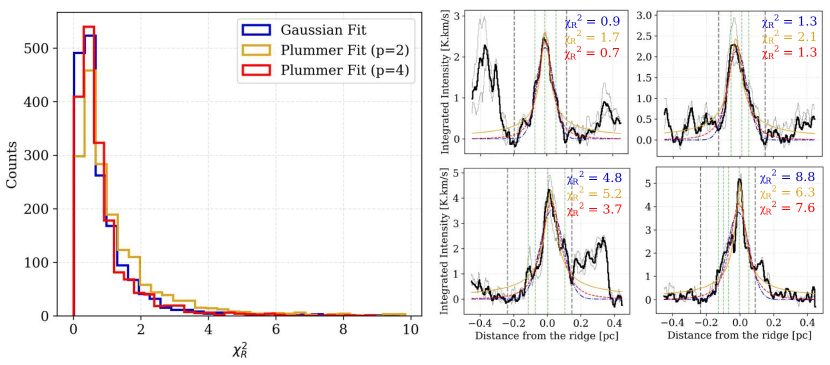
In order to assess the goodness of our radial intensity profile fits we calculate the reduced chi-squared values for each individual fit and for the three different methods that we employed. The reduced chi-squared is simply calculated as chi-squared per degree of freedom. The resulting distributions of reduced chi-squared of all the fits are shown in the left panel of Figure 7. The median reduced chi-squared values of our fits are 0.6 for the Gaussian and Plummer p=4 fits, and 0.8 for the Plummer p=2 fits. The reduced chi-squared value for a good fit is expected to be close to 1. However, by inspecting the intensity profiles and their corresponding reduced chi-squared values, we see that with the reduced chi-squared values up to 6, the fits still describe the underlying intensity profiles well. The right panel of Figure 7 shows four different intensity profiles, overlaid with the calculated fits and the corresponding reduced chi-squared values for each fit. In both panels of the figure, blue, yellow, and red colors represent the Gaussian, Plummer with p=2 and Plummer with p=4 fits. Profiles with blending structures or extended shoulders such as the example shown in the bottom right subplot leads to poor fits with high reduced chi-squared (${\chi}_{R}^{2}>$ 6). For the Gaussian fits, 98% of the reduced chi-squared values lie between 0 and 6, while this value is 97% for the Plummer p=2 and 99 % for Plummer p=4 fits. We confirm by eye that the tail of the reduced chi-squared distribution (${\chi}_{R}^{2}>$ 6) corresponds to questionable fits. The reason for this is the complexity of the intensity profiles. As the width of these profiles are hard to estimate, they are discarded from further analysis. We note that the reduced chi-squared criterion applies for the Gaussian and Plummer fits individually; i.e. a profile can have a good reduced chi-squared for Plummer p=2 fit but not for the Gaussian, and in this case only the Plummer p=2 width is accounted for. As we do not have a reduced chi-squared value for the widths calculated from the second moment method, we take those second moment widths where the reduced chi-squared criterion is satisfied in all the other three methods.

Figure 7: Left: ${\chi}_{R}^{2}$ values for each radial intensity profile fit for the different methods used in the width determination. Right: Four examples of profiles with different reduced chi-squared values. The bottom right sub-panel shows the example of a fit discarded due to its large reduced chi-squared.

3.2.2 Dependence on the fitting range

Arzoumanian et al. (2011) and later studies of filaments (e.g. André et al. 2016; Federrath et al. 2016) refrain from fitting the wings of the column density profiles, and the fitted inner range of the profiles is always the same for each and every column density slice. Smith et al. (2014) and Panopoulou et al. (2017) show that a correlation between the fitting range and the calculated width of these profiles exists. This correlation is not unexpected. Depending on the portion of the profiles that is fitted, the larger the fitted area, the wider the width of the profile will be. This behavior arises from the fact that the filament profiles are not isolated. Therefore, the larger the fitting range, the more emission the function will try to fit. In an ideal case, where the baseline was perfectly smooth, the fitting range should not affect the width of the distribution. In real observed data, however, the filament profile is accompanied by extended emission as well as emission from nearby filaments and hubs. Hence, a linear correlation between the fitting range and the resulting width is inevitable. To be as independent of this bias as much as possible, instead of forcing a fixed boundary for our fits, we calculate a unique fitting range for every individual profile. This is done automatically within FilChaP by looking for minima around the peak intensity of the filament. If the minima have a significance of 3 beam sizes (which corresponds to a well resolved nearby or blended structure) their locations mark the boundaries for the fitting range. In this approach, each profile has its own fitting range which depends on the filament’s environment.

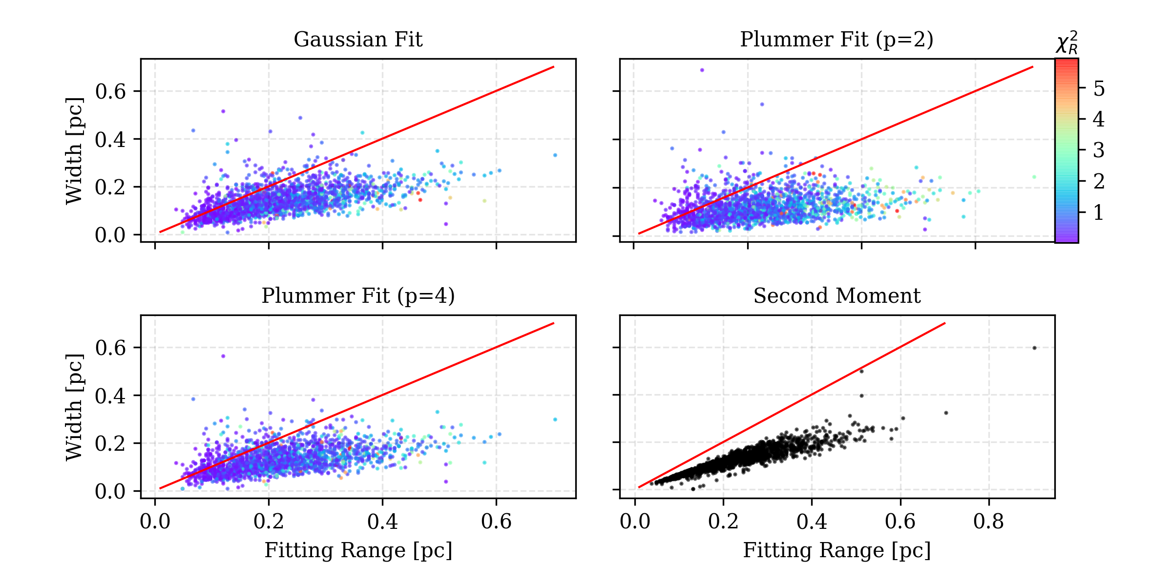
Figure 8 shows the the correlation between the fitting ranges for each individual profile and the derived widths based on the 4 different methods. The scattered points are colored by the ${\chi}^{2}$ of each fit, except for the second moment widths, as those are not fitted but calculated directly from the distribution. The red diagonal lines correspond to a 1-1 relation between the two axes. The strongest correlation between the fitting range and the width is for the case of the second moment (bottom right panel). This is purely because the second moment is calculated based on the boundaries of the distribution, so that the larger the distance between the boundaries the larger is the width. As is also seen from this panel, the second moment width of the distribution cannot be larger than the fitting range. For the Gaussian and Plummer fits, the widths can occasionally be larger than the fitting range, these are the points that lay above the 1-1 correlation line. These points are excluded from the analysis as they originate from profiles with multiple peaks that are not straightforward to analyze.

Of the four different methods used to calculate the filament widths, the Plummer (p=2) fit seems to be the most independent of the fitting range as it shows the shallowest increase with the increasing fitting range. However, as can be seen in the various intensity profiles shown in Figures 3 and 7, the Plummer (p=2) only fits the very inner portion of the profile. This is acceptable when one has multiple peaks, but it excludes the information on the wings of the profile. This is the reason why the widths calculated from the Plummer (p=2) are always narrower and less dependent on the fitting range than the ones estimated from the other methods. Furthermore, because it fits a substructured profile better, it has fewer points above the 1-1 relation between the fitting range and width. However, we refrain from drawing conclusions of filaments’ state of isothermality based on the power-law indices of the Plummer fits, because the difference between the p=2 and p=4 seem to be sensitive to, at least in this work, the amount of background emission observed towards individual filaments.

Figure 8: Correlation between the calculated filament widths and the fitting range on the radial intensity profile over which the width is calculated. The red diagonal line shows the 1-1 correlation between the two parameters. The strongest correlation is observed when instead of the fits, the second moment of the distribution is used. The color bar indicates the reduced chi-squared values for the fits. There is also a slight correlation between the reduced chi-squared and the fitting range.

4 Discussion

4.1 Variation of the filament width across the cloud

As shown in Figure 6 we see that the filament width varies even along a single filament. This variation is often caused by blending structures. Close to hubs – where filaments meet, the intensity profiles get wider as many structures merge into one another. We follow the variation of width along each filament by plotting the width (Gaussian FWHM) on the C¹⁸O map. This spatial variation is shown on the left hand side of Figure 9 with the points along each filament colored by the width calculated at that point. The corresponding colorbar indicates the calculated width. In order to demonstrate the complexity of the radial intensity profiles we also calculate the number of shoulders identified in each profile. The shoulders appear as bumps within the boundaries within which we calculate the width of the filaments, further proving that these radial profiles are not simple single-component Gaussians. Examples of the intensity profiles with detected shoulders are shown in the right hand panels of Figure 7. In this example, the boundaries are shown with the grey dashed lines that clearly separate the emission of the filament from a nearby structure that appears at around 0.2 pc (bottom right subplot). The green dashed lines indicate the locations of the detected shoulders that correspond to bumps within the filament profile that are not significant enough to be separate structures. Up to this point, we have qualitatively shown that filament profiles are substructured and complex which in turn leads to variation of filament widths. A possible correlation between the number of shoulders, the locations of filaments, and the filament widths would indeed allow us to study this phenomenon quantitatively. We plot the identified filaments on the C¹⁸O peak intensity map, this time with each point colored by the number of shoulders detected in the corresponding intensity profile. Figure 9 shows how this number changes along the filaments and across the cloud.

Figure 9: Filament width (left panel) and number of shoulders (right panel) for the filaments idnetified in Orion A overlayed on the C¹⁸O peak intensity map. The color of each point along filaments represents the width (left) and the number of shoulders (right) at that point, corresponding to the colorbar shown in the right side of the panels. The arrows indicate the positions of hubs where filaments converge.

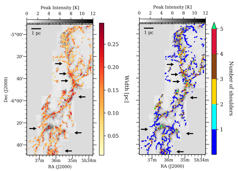
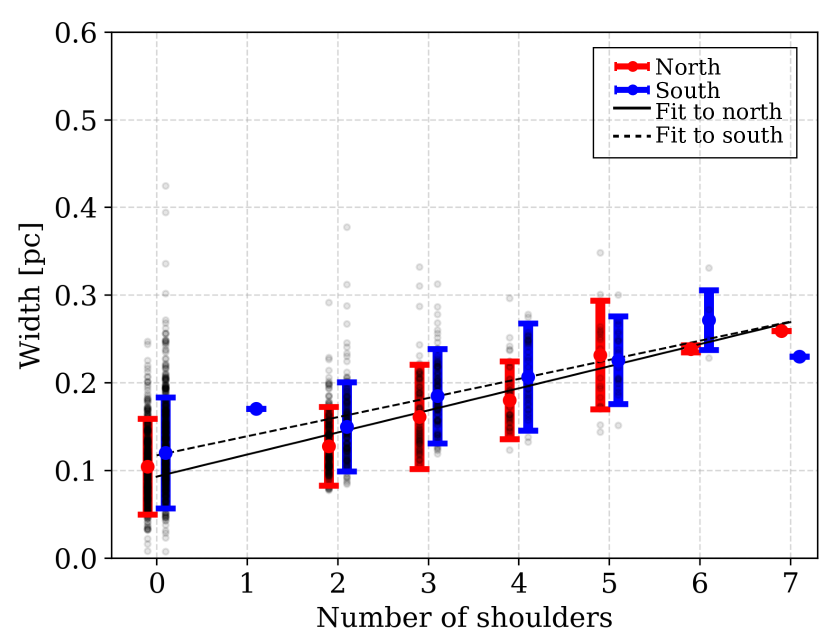
Figure 9 suggests a clear correlation between the filament width and the number of shoulders. To demonstrate this correlation better, in Figure 10 we show the detected number of shoulders plotted against the corresponding widths of each individual profile. The data points are plotted as grey circles, and their median values are shown as red and blue filled circles for the northern and the southern regions of the map, respectively. The error bars on the median values indicate the interquartile range. The majority of the filament profiles have at least 1 shoulder detected. The existence of such highly complex intensity profiles implies that filaments are not perfectly isolated cylinders, but that they have substructures within them. Figure 10 clearly shows that there is a linear correlation between the number of shoulders and the width: the higher the number of shoulders, the wider is the calculated width. Clarke et al. (2017) suggest that filaments may retain wide widths even when supercritical, due to substructure. This substructure lessens the global effects of gravity and produces wider filaments. The linear correlation we find in Figure 10 supports this view. This correlation suggests widths of 0.09$\pm$0.02 pc and 0.12$\pm$0.01 pc for filaments without shoulders, for the northern and southern region, respectively.

4.2 The lack of correlation between filament width and column density

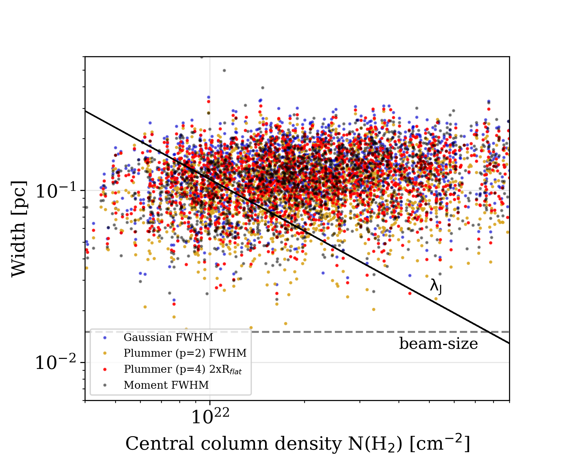
To account for the variation of the filament width throughout the ISF, we also checked for a possible (anti-)correlation between the column density along the filaments and their width. Figure 11 shows the central column density at every point along the spine of the filaments plotted against the corresponding width at that point. The column density of each pixel along the identified filaments is taken from the Herschel dust column density map published in Stutz & Kainulainen (2015). Blue, yellow, red and black colored points in the plot represent widths derived Gaussian fits, Plummer p=2 and p=4 and the second moment, respectively. The dashed line is the resolution of the observations, and the solid diagonal line is the thermal Jeans length at 10 K; $\lambda_{J}=c_{s}^{2}/G\mu_{H}\Sigma_{0}$ where $\Sigma_{0}$ is the central column density (Arzoumanian et al. 2011). Ideally, if the filaments are super-critical, and thus gravity-dominated (right hand side of the $\lambda_{J}$ line), they would contract to fragment and form cores, hence leading to an anti correlation between the width and the central column density. However, this does not appear to be the case. This lack of anti correlation has been found by Arzoumanian et al. (2011) in low-mass star forming regions; Aquila, IC5146 and Polaris. We confirm that even in a high-mass star forming region that is as active and complex as Orion A, the decoupling of filament widths from the central column densities of the filament spine persists. We propose the width variation along filaments is indeed mostly regulated by environmental effects, i.e. their positions relative to the hubs and whether the filaments are rather isolated or are connected to or disconnected from surrounding structures.

Arzoumanian et al. (2011) speculated that the decorrelation of the width and central column density can be explained with turbulent filament formation through compression (e.g. Padoan et al. 2001) for the sub-critical filaments, and the super-critical filaments may be able to maintain an approximately constant width if they are continuously accreting from their surroundings. Following this work, Heitsch (2013) studied gravitational infall onto isothermal filaments that are subject to external pressure to see for which conditions the filament width can be independent of the column density. Their best model that fits the lack of correlation seen in observations is for the magnetized filaments that are subject to varying external pressure due to ram pressure exerted by the infalling material. Our results in Figure 11 can be directly compared to the results in Heitsch (2013), particularly their Figure 4. Even though their best fitting model represents the majority of our data points, we do not see a decrease in filament width towards higher column densities up to 10²³ cm^-2 as the model predicts.

Figure 10: Variation of the filament width with respect to detected number of shoulders in the corresponding intensity profile. The gray circles represent the data points, the red and blue filled circles are the median values. The shown error bars on the median values represent the interquartile range.

Figure 11: Filament widths calculated using the four different methods plotted against the central column density at each point where the width is calculated. The colors represent FWHM of Gaussian fits (blue), moment analysis (black), Plummer p=2 (yellow) and p=4 (red). The dashed line represents the resolution of our observations and the solid diagonal line the thermal Jeans length at 10 K.

5 Conclusions

We present a study of the filament properties in the Orion A molecular cloud as seen in the emission of the dense gas tracer C¹⁸O, produced by the CARMA-NRO Orion Survey (Kong et al. 2018). We identified 625 filaments in the 3D datacube (PPV) using the DisPerSE algorithm. In this first paper, which will be followed by a series of papers including the analysis of filament kinematics and filament properties in different tracers (¹³CO, dust and C⁺), we investigated the physical properties of filaments with an emphasis on the filament width.

Based on the shortcomings of the methods that led to the identification of a “universal” filament width, criticized in previous works by Smith et al. (2014) and Panopoulou et al. (2017) we developed an improved and automated method to study characteristics of filaments; FilChaP, a python based algorithm. In this method, while calculating the filament widths: (i) the radial intensity profiles are not averaged over the length of an entire filament, but over a number of consecutive slices that represent a region 3 beam-sizes in length, (ii) there is no fixed fitting range for these profiles that would force a prefixed width. Instead, each profile has its own fitting range. This range is set by the minima around the peak emission from the filament. The minima are required to have a significance of 3 beam-sizes, (iii) we use 4 different methods to derive filament widths; with a Gaussian fit, two Plummer-like fits with p=2 and p=4, and the FWHM derived from the second moment of the intensity distribution and (iv) we judge the goodness of each fit by looking at their reduced chi-squared values to prevent ‘poor’ fits biasing the results. We find the following key points:

• The median filament widths are $0.14\begin{subarray}{c}+0.03\\ -0.02\end{subarray}$ pc and $0.16\begin{subarray}{c}+0.04\\ -0.03\end{subarray}$  pc for the Gaussian fits, $0.11\begin{subarray}{c}+0.03\\ -0.02\end{subarray}$  pc and $0.13\begin{subarray}{c}+0.04\\ -0.03\end{subarray}$  pc for the Plummer p=2 fits, $0.13\begin{subarray}{c}+0.03\\ -0.03\end{subarray}$  pc and $0.14\begin{subarray}{c}+0.03\\ -0.03\end{subarray}$  pc for the Plummer p=4 fits, and finally, $0.13\begin{subarray}{c}+0.03\\ -0.03\end{subarray}$  pc and $0.14\begin{subarray}{c}+0.04\\ -0.03\end{subarray}$  pc for the FWHM derived from the second moment for the northern and southern regions, respectively.

• The width, regardless of the method used, is not correlated with the central column density. Although there is more than an order of magnitude scatter in width, neither sub nor super-critical filament widths are coupled to the column density. The Heitsch (2013) model with magnetized and externally pressured filaments best reproduces the observed decorrelation.The model agrees with our observations except for high column densities (10²³ cm^-2) where narrower widths are predicted. We found that even at these high column densities traced by our filaments the lack of correlation persists, however, we note that we have a statistically smaller sample at the higher column density end. Accreting filaments in a magnetized environment similar to Heitsch (2013) model have already been observed in Taurus (e.g. Palmeirim et al. 2013) with striations of material perfectly aligned with the magnetic field surrounding the main filament. A similar analysis using, e.g. BISTRO polarization data (Pattle et al. 2017) can be conducted with the CARMA-NRO Orion Survey data in a future study.

• Given the lack of correlation with the column density, we attribute the gradient of the widths all across the cloud to the fact that the filaments are not isolated, homogeneous structures. They are composed of substructure, surrounded by nearby filaments and they form hubs. Connected and disconnected filaments have fluctuating widths. We find that the majority of filaments closer to the star forming hubs have larger widths. We quantify the complexity of the intensity profiles by looking at the number of shoulders that each profile has. This examination reveals a linear relation between the filament widths and the number of shoulders. From this linear relation we obtain widths of 0.09$\pm$0.02 pc and 0.12$\pm$0.01 pc for a filament with no substructure in northern and southern Orion A, respectively. We suggest that the complexity of the intensity profiles contribute significantly to the spread of the filament width distribution.

• The majority of the identified filaments do not resemble the fibers reported in a study towards the Taurus molecular cloud which spatially overlap but are distinct coherent structures in velocity space along the line-of-sight (Hacar et al. 2013). The only fiber-like filaments we find are located in the OMC-4 region where we observe clear multiple velocity components along the line of sight that form coherent structures. The fact that the filaments identified in N₂H⁺ towards the northern ISF by Hacar et al. (2018) and the majority of the filaments identified in this study do not show a spatial overlap implies that the general picture of the filamentary structure in Orion A may differ from what has been observed towards the low mass star forming region Taurus.

Appendix A FilChaP: Filament Characterization Package

FilChaP is a python-based software package that can be used to characterize physical properties of filaments. FilChaP derives radial intensity profiles perpendicular to filament spines from which it calculates filament width, skewness and kurtosis. In addition, FilChaP can also calculate filament length and curvature, as well. The algorithm is publicly available for download at https://github.com/astrosuri/filchap. The download folder includes a python tutorial with an example filament skeleton and a 3D fits cube which the users can utilize to run FilChaP and derive filament properties. The version of FilChaP used to produce the results in this paper has a specific DOI (https://doi.org/10.5281/zenodo.2222325) and is archived on Zenodo.

FilChaP requires filament coordinates as an input file to derive information on filaments. For this particular study, we have used the output filaments of DisPerSE. These output filaments are simple ASCII files indicating filament ID, x-coordinate (RA), y-coordinate (DEC), z-coordinate (velocity channel). These 4 parameters are given for each point along a filament. If the filaments are identified on a 2-dimensional map instead, then the z-coordinate that corresponds to the velocity channel does not exist in the output file and is not required by FilChaP, and the code can be used in 2D mode.

The filament width calculation method, as it is the main focus of this study, is explained thoroughly in Section 3.1. Below we explain the baseline removal method used, and present ‘synthetic’ filament networks which we constructed with known widths for the purpose of testing FilChaP.

A.1 Baseline Subtraction

FilChaP uses Asymmetric Least Squares Smoothing (AsLS) method for baseline subtraction (Eilers 2005). A commonly used way of achieving a baseline is to smooth the profile until peaks or dips of interest are no longer prominent. The most common smoothing method is the least square method which minimizes the deviations of the smooth counterpart $h$, from the noisy data, $f$. The least square method weighs both negative and positive deviations of $h$ from $f$ the same. In the AsLS method however, deviations from the estimated baseline are weighted asymmetrically, with the positive deviations being weighted less. Because if $f-h$ is a good representation of $f$’s baseline, the deviations should always be positive ($f>h$) due to the fact that $f$ will always have signal (peaks) that take values higher than $h$.

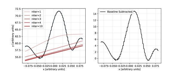
Figure 12 shows an example of the baseline subtraction process. On the left panel a representative intensity profile with a baseline gradient is shown. This gradient has to be removed before FilChaP can fit a function to calculate its FWHM. The different shades of solid red lines represent the AsLS baselines, $h$, calculated at different number of iterations. After only a few iterations the calculated weights quickly converge, hence a final baseline is obtained. The right panel of the plot shows the baseline subtracted profile. Eilers (2005) gives a MATLAB code for the iterative process of calculating the baselines, and this code is converted to python under https://stackoverflow.com/questions/29156532/python-baseline-correction-library/29185844. This python code is used by FilChaP. One possible drawback of the AsLS method is that once the baseline is removed a portion of the emission could go below zero. In the future we plan to use STATCONT to prevent this (Sánchez-Monge et al. 2018).

Figure 12: Example baseline subtraction process. Left: Data with a baseline gradient is shown with the black solid curve. The curves with different shades of red represent the AsLS baselines calculated with different number of iterations. The solutions for the baseline converge rather quickly within 10 iterations. Right: The baseline subtracted profile.

A.2 Tests on the width calculation method

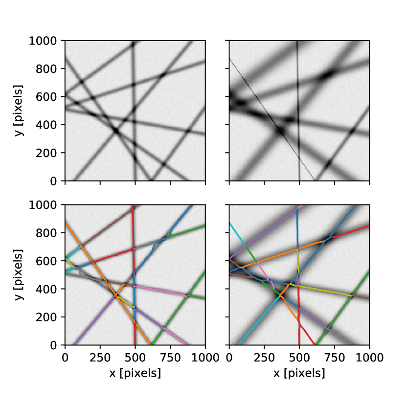
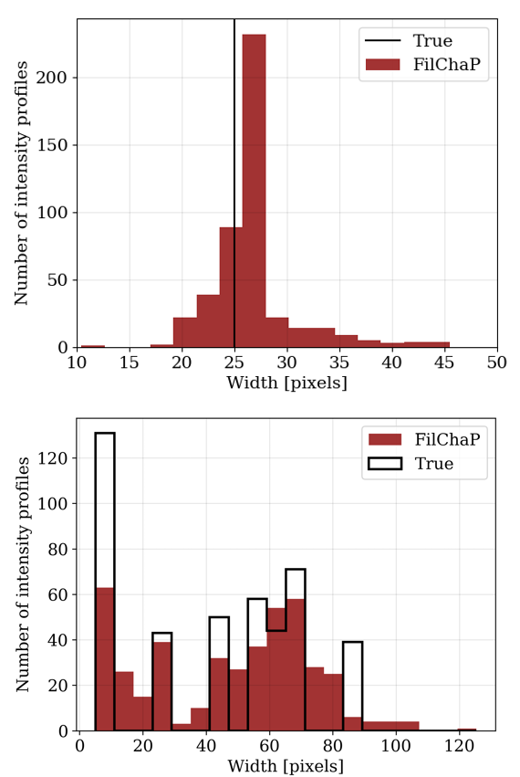
Figure 13 shows the generated filaments width equal widths (Case 1; top left), and unequal widths (Case 2; top right). The exercise here is to see whether in two different cases, (1) where all filaments have the same width and (2) where all filaments have a different width, FilChaP can recover the width distribution. Both cases have an amount of random Gaussian noise that is selected based on the peak intensity-to-noise ratio in our C¹⁸O integrated intensity map. In Case 1, all the filaments have a 25 pixel width. In the C¹⁸O map, 25 pixels correspond to a 0.1 pc filament width in spatial scales. For Case 2, we allow filament width to vary between 5 and 85 pixels. This is to assess FilChaP’s performance in detecting extreme cases of narrow filaments and diffuse filaments. While for Case 1 we expect to find a distribution that is strongly peaked at around 25 pixels, for Case 2 we expect a wide distribution that has the contribution from all the different scales from 5 pixels to 85 pixels. Figure 14 shows the FilChaP width calculation result for Case 1 (top panel) and Case 2 (bottom panel). As anticipated, the width distribution for Case 1 has a narrow peak, with a mean of 26.5$\pm$4.2 pixels (where the error corresponds to the 95% confidence level). For Case 2, we plot both the true input distribution of filament widths and the FilChaP output distribution. In order to quantify the association between the input and output width distributions for Case 2, we calculate Spearman’s rank correlation coefficient. This coefficient gives a non-parametric measure of the relation between the two distributions which are connected with a monotonic function. The coefficient takes values between -1 and +1, where the coefficient takes a value of -1 in case of a perfect decreasing monotonic correlation, +1 in case of an increasing monotonic correlation and 0 in case of no correlation. The Spearman’s rank coefficient between our the two distributions of Case 2 is 0.77; indicating a strong link between the two datasets. It is clear that the spread of the distribution for Case 1 comes from the errors of individual fits, and the fact that the filaments cross each other at various points throughout the map, which in turn introduces larger widths. For Case 2, in addition to large filament widths at crossing points and the fitting errors, the large spread comes from the underlying dissimilarities between the filament widths. In comparison, the two different cases produce significantly different width distributions that FilChaP successfully captures.

Figure 13: Top: Synthetic filamentary network generated with prefixed filament widths on a $1000\times 1000$ pixel grid. On the left, all the filaments have a same width of 25 pixels, while on the right, each filament has a different width that vary from 5 to 85 pixels (see Fig. 14). Bottom: Filaments identified by DisPerSE.

Figure 14: Distribution of filament widths for the test two cases presented in Figure 13. For Case 1 (top panel) the input widths of all the filaments are 25 pixels (solid black line) and the mean of the width distribution calculated with FilChap is 26.5$\pm$4.2 pixels. For Case 2 (bottom panel), the true distribution of the input filament widths is given with the black histogram, and the width calculation that results using FilChap is given with the red histogram. The Spearman correlation coefficient between the two datasets is 0.77.

A.3 Additional functions

In addition to the filament width, FilChaP calculates filament skewness, kurtosis, length and curvature. The second moment of the intensity profiles is calculated to assess their FWHM, along with the second moment, the third and fourth moments; skewness and kurtosis are also calculated within the width calculation function of FilChaP. The length and curvature are calculated in separate functions, based on the filament spines extracted using DisPerSE.

A.3.1 Skewness and kurtosis

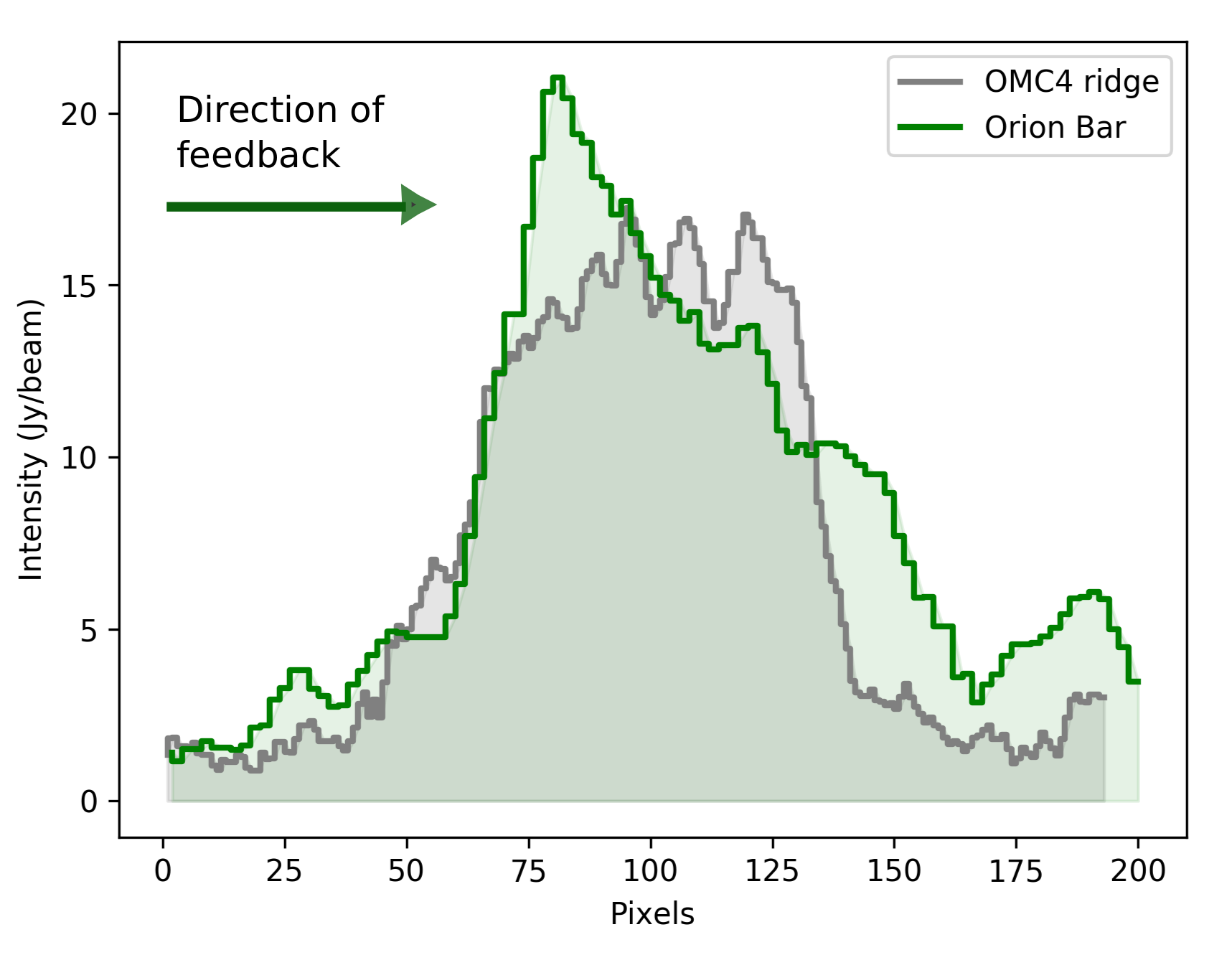
The skewness and kurtosis provide information about the shape of the intensity profiles. This shaped can be related to physical properties of the filaments and their environments. For example, if a filament is in a feedback region, we expect the intensity profile to be sharper on the side where the filament faces the direction of the feedback. Kurtosis, on the other hand, is a measure of peakiness. Therefore it can indicate locations of high-density, as the CO isotopologues may get optically thick, or in case of C¹⁸O, freeze out that causes the profiles to flatten in the top. Figure 15 demonstrates how we can detect the variations of skewness and kurtosis in Orion A. The two plotted intensity profiles are calculated from the ¹³CO emission map and show slices accros the Orion Bar, a well known PDR and OMC-4, the dense star forming region, in green and grey, respectively. The direction of the feedback to the PDR from the Trapezium cluster is shown with a green arrow. The side of the PDR profile towards the feedback forms a sharp edge, whereas the side away from the feedback extends slowly. The OMC-4 ridge shows no such skewness as it is much less affected from the feedback. This plot also shows the difference between the peakiness of both profiles, which can then be quantified with the kurtosis parameter. The following paper on comparing filament properties in different tracers (Suri et al. in prep) touches upon the PDR nature of the filaments in feedback regions and compares properties of intensity profiles using skewness and kurtosis analysis.

Figure 15: Comparison of two intensity profiles with different values of skewness and kurtosis. The intensity profile for the Orion Bar position is positive skewed with a tail to the right, while the intensity profile of the OMC4 ridge position is flat in the top resulting in a platykurtic or negative kurtosis distribution. FilChaP determines the skewness and kurtosis of the filament intensity profiles.

A.3.2 Length and curvature

In order to obtain the filament length, FilChaP calculates the projected distances between the consecutive skeleton points along a filament. This is a projected distance, because in observational datasets we do not have a knowledge on the spatial 3rd dimension of the filaments. In addition, the code offers calculating “kinkiness”, or in other words; curvature, of filaments by comparing the calculated length of the filament to the distance between the start and end points. Therefore, we define curvature as $k=r/R$ where $r$ is the distance between the end points and $R$ is the calculated length of the filament. A $k$ value of unity indicates a straight filament.

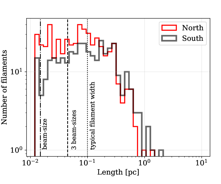
These two properties of filaments; length and curvature, are highly dependent on the parameters used to identify filaments with DisPerSE. Therefore, we note that the resulting statistics should be interpreted with caution. However, the credibility of these parameters can be improved in the future by testing different filament identification methods, comparing identified filamentary structures to one another, and using multiple tracers to assess the connection. Nevertheless, for the identified filaments in C¹⁸O using DisPerSE with the set of parameters explained in Section3, we measured filament length between 0.03-1.8 pc. Figure 16 shows the distribution of the resulting filament lengths for the northern (red) and southern Orion A (black). The dashed vertical line at 0.045 pc indicates 3-beamsizes, and for the width calculations we discard the structures that are shorter than 0.045 pc.

Figure 16: Distribution of filament lengths in the north (red) and south (black). The dot-dashed, dashed and the dotted lines respectively indicate a beam-size, 3 beam-sizes and the typical filament width found in this study.

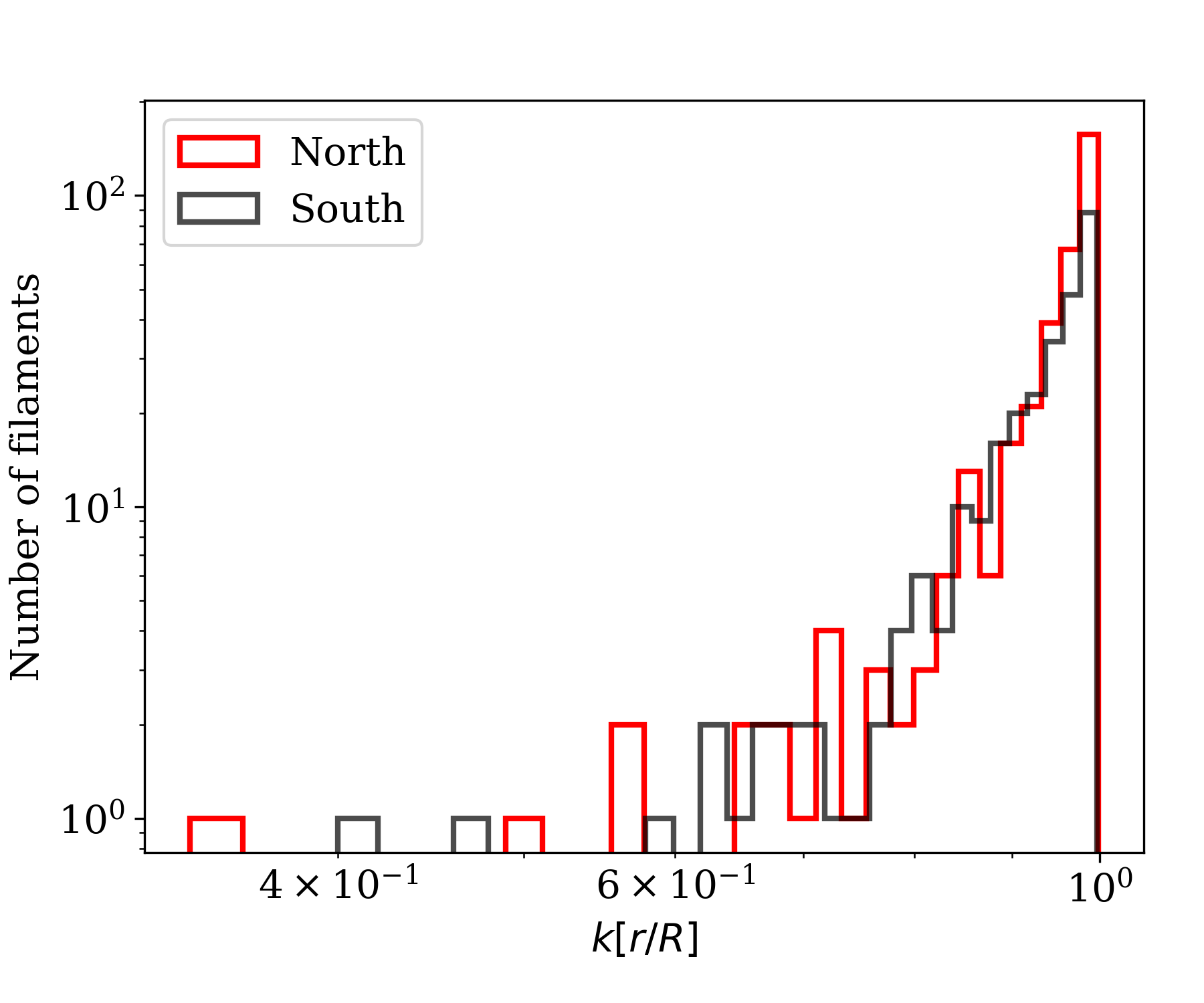
The curvature values of filaments in Orion A north and south are shown in histograms in Figure 17. There are a few filaments that appear to be more bent, and have $k$ values of between 0.3–0.9. The most bent filament in the north is located in OMC4 ridge. Majority of filaments, however, have very low curvature.

Figure 17: Distribution of filament kinkiness, $k$, where $k=r/R$ with $r$ being the distance between the end points and $R$ the calculated length of the filament. The majority of the filaments in Orion A are found to be unbent.

Appendix B Additional Material

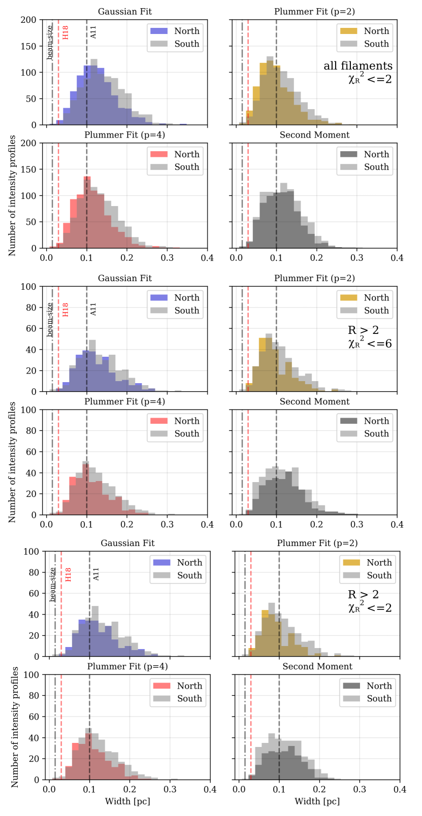
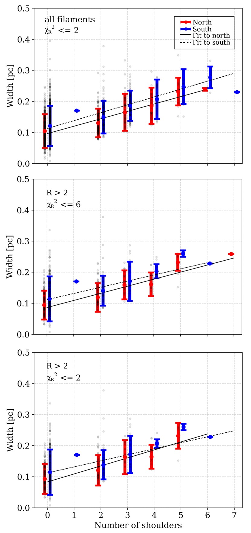
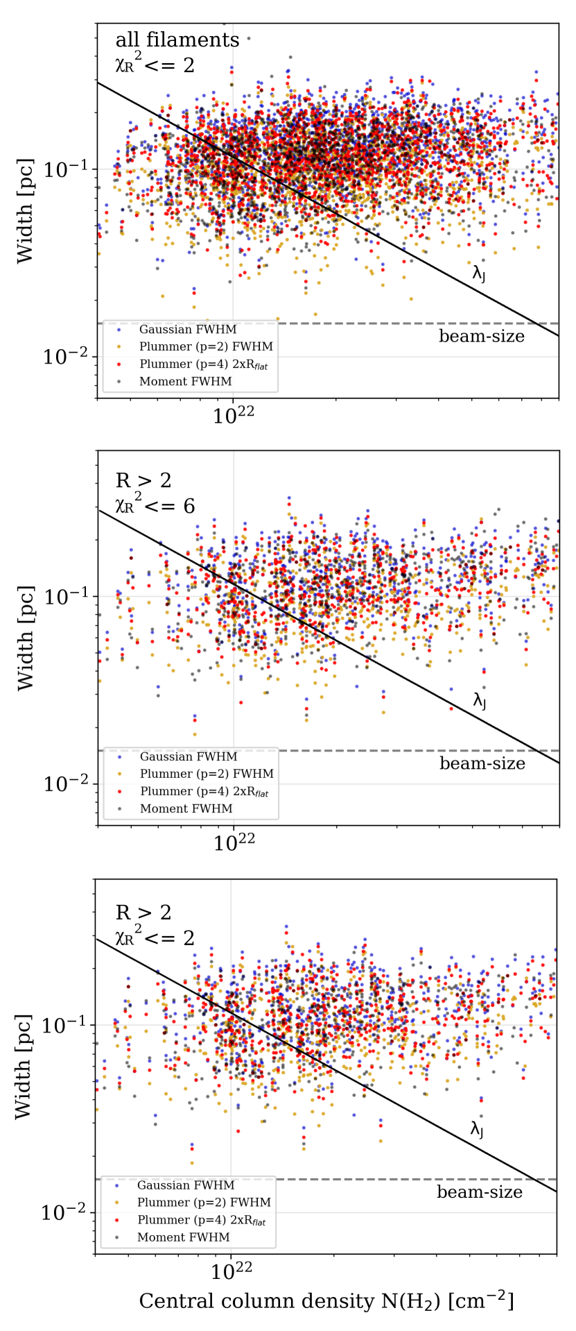
In Section 3, we presented width distributions for all the identified filaments that are longer than 3 beam-sizes and are fitted with a reduced chi-squared less than 6. Here, we reproduce Figures 5, 10 and 11 considering different criteria on filament and profile selection. We look at the width distributions of (1) all filaments and intensity profiles fitted with a reduced chi-squared less than or equal to 2, (2) filaments with aspect ratios larger than 2 and intensity profiles that are fitted with a reduced chi-squared less than or equal to 6, (3) filaments with aspect ratios larger than 2 and intensity profiles fitted with a reduced chi-squared less than or equal to 2. This different selection criteria are aimed to ensure that we do not introduce any bias in the determined widths when including all the filaments that are longer than 3 beam-sizes and have a reduced chi-squared less than 6.

Figure 18: Width distributions for four different width calculation methods (Gaussian, Plummer-like with p=2 and p=4 and second moment, as shown in Fig. 5) when the filament aspect ratio and the reduced chi-squared criteria are varied. The top four panels show the distributions of all filaments and intensity profiles fitted with a reduced chi-squared less than or equal to 2. The middle four panels show the width distributions for filaments with aspect ratios larger than 2 and fits with chi-squared less than or equal to 6. Finally, the bottom four panels show the width distributions for filaments with aspect ratios larger than 2 and reduced chi-squared values less than or equal to 2.

Figure 19: Same as Figure 10 for the different criteria (aspect ratio and reduced chi-squared of the fit) studied in Section B.

Figure 20: Same as Figure 11 for the different criteria (aspect ratio and reduced chi-squared of the fit) studied in Section B.

Table 1: Median filament widths according to different selecting criteria (see Figure 18), and inferred filament width when no shoulders are identified in the intensity profile (intercept of the linear fits of Figure 19).

Criteria	Gaussian	Plummer (p=2)	Plummer (p=4)	Second Moment	Intercept
	north/south	north/south	north/south	north/south	north/south
all, ${\chi}_{R}^{2}\leq$ 6	$0.12\begin{subarray}{c}+0.15\\ -0.09\end{subarray}$ pc	$0.09\begin{subarray}{c}+0.13\\ -0.07\end{subarray}$ pc	$0.11\begin{subarray}{c}+0.14\\ -0.08\end{subarray}$ pc	$0.12\begin{subarray}{c}+0.15\\ -0.09\end{subarray}$ pc	0.09$\pm$0.02 pc
	$0.14\begin{subarray}{c}+0.18\\ -0.11\end{subarray}$ pc	$0.11\begin{subarray}{c}+0.14\\ -0.08\end{subarray}$ pc	$0.13\begin{subarray}{c}+0.16\\ -0.09\end{subarray}$ pc	$0.12\begin{subarray}{c}+0.15\\ -0.09\end{subarray}$ pc	0.11$\pm$0.01 pc
all, ${\chi}_{R}^{2}\leq$ 2	$0.12\begin{subarray}{c}+0.15\\ -0.09\end{subarray}$ pc	$0.09\begin{subarray}{c}+0.12\\ -0.07\end{subarray}$ pc	$0.11\begin{subarray}{c}+0.14\\ -0.08\end{subarray}$ pc	$0.11\begin{subarray}{c}+0.14\\ -0.08\end{subarray}$ pc	0.10$\pm$0.01 pc
	$0.14\begin{subarray}{c}+0.18\\ -0.11\end{subarray}$ pc	$0.11\begin{subarray}{c}+0.14\\ -0.08\end{subarray}$ pc	$0.12\begin{subarray}{c}+0.16\\ -0.10\end{subarray}$ pc	$0.12\begin{subarray}{c}+0.15\\ -0.08\end{subarray}$ pc	0.11$\pm$0.01 pc
R ¿ 2, ${\chi}_{R}^{2}\leq$ 6	$0.12\begin{subarray}{c}+0.15\\ -0.09\end{subarray}$ pc	$0.09\begin{subarray}{c}+0.12\\ -0.07\end{subarray}$ pc	$0.10\begin{subarray}{c}+0.14\\ -0.08\end{subarray}$ pc	$0.12\begin{subarray}{c}+0.15\\ -0.09\end{subarray}$ pc	0.09$\pm$0.02 pc
	$0.13\begin{subarray}{c}+0.17\\ -0.09\end{subarray}$ pc	$0.10\begin{subarray}{c}+0.14\\ -0.08\end{subarray}$ pc	$0.12\begin{subarray}{c}+0.15\\ -0.09\end{subarray}$ pc	$0.11\begin{subarray}{c}+0.15\\ -0.08\end{subarray}$ pc	0.11$\pm$0.01 pc
R ¿ 2, ${\chi}_{R}^{2}\leq$ 2	$0.11\begin{subarray}{c}+0.15\\ -0.09\end{subarray}$ pc	$0.08\begin{subarray}{c}+0.12\\ -0.06\end{subarray}$ pc	$0.10\begin{subarray}{c}+0.14\\ -0.08\end{subarray}$ pc	$0.11\begin{subarray}{c}+0.15\\ -0.08\end{subarray}$ pc	0.08$\pm$0.03 pc
	$0.12\begin{subarray}{c}+0.17\\ -0.09\end{subarray}$ pc	$0.10\begin{subarray}{c}+0.13\\ -0.07\end{subarray}$ pc	$0.12\begin{subarray}{c}+0.15\\ -0.08\end{subarray}$ pc	$0.11\begin{subarray}{c}+0.15\\ -0.08\end{subarray}$ pc	0.11$\pm$0.01 pc

The width distributions for the cases mentioned above are shown in Figure 18 top, middle and bottom panels, respectively. For the majority of the cases, regardless of the criteria, the southern region of Orion A has filaments with larger widths as found in Fig. 5. The distribution of Plummer-like (p=2) fits results in the most narrow median filament width ($0.08\begin{subarray}{c}+0.12\\ -0.06\end{subarray}$ pc) when only those filaments with an aspect ratio larger than 2 and a reduced chi-squared value less than 2 is selected. The median filament widths for these three cases in the northern and southern regions are listed in Table 1. The median widths in all cases are in the range 0.08 pc to 0.14 pc, similar to the range found when considering all the filaments.

In Fig. 19, we reproduce the correlation between the filament width and the number of shoulders for the varying selection criteria considered above (i.e., aspect ratio and reduced chi-squared). Similar linear fits are found in all cases. The inferred filament width when no shoulders are identified in the intensity profiles for each of the cases considered is listed in the last column of Table 1.

Finally, in Fig. 20 we investigate that the no correlation found between filament widths and H₂ column density is not biased by the selection of the filaments. The bottom panel in Fig. 20 is the most strict selection of filaments (filaments with aspect ratio larger than 2 and reduced chi-squared less than 5) suggest no correlation between width and column density as discussed when considering all the filaments.

References

- André (2017) André, P. 2017, Comptes Rendus Geoscience, 349, 187
- André et al. (2010) André, P., Men’shchikov, A., Bontemps, S., et al. 2010, A&A, 518, L102
- André et al. (2016) André, P., Revéret, V., Könyves, V., et al. 2016, A&A, 592, A54
- Arzoumanian et al. (2011) Arzoumanian, D., André, P., Didelon, P., et al. 2011, A&A, 529, L6
- Bally et al. (1987) Bally, J., Langer, W. D., Stark, A. A., & Wilson, R. W. 1987, ApJ, 312, L45
- Chira et al. (2018) Chira, R.-A., Kainulainen, J., Ibáñez-Mejía, J. C., Henning, T., & Mac Low, M.-M. 2018, A&A, 610, A62
- Clarke & Whitworth (2015) Clarke, S. D. & Whitworth, A. P. 2015, MNRAS, 449, 1819
- Clarke et al. (2017) Clarke, S. D., Whitworth, A. P., Duarte-Cabral, A., & Hubber, D. A. 2017, MNRAS, 468, 2489
- Clarke et al. (2016) Clarke, S. D., Whitworth, A. P., & Hubber, D. A. 2016, MNRAS, 458, 319
- Duarte-Cabral & Dobbs (2016) Duarte-Cabral, A. & Dobbs, C. L. 2016, MNRAS, 458, 3667
- Eilers (2005) Eilers, P. H. and Boelens, H. F. 2005, J. Raman Spectrosc.
- Federrath et al. (2016) Federrath, C., Rathborne, J. M., Longmore, S. N., et al. 2016, ApJ, 832, 143
- Fiege & Pudritz (2000) Fiege, J. D. & Pudritz, R. E. 2000, MNRAS, 311, 85
- Fischera & Martin (2012) Fischera, J. & Martin, P. G. 2012, A&A, 542, A77
- Grossschedl et al. (2018) Grossschedl, J. E., Alves, J., Meingast, S., et al. 2018, ArXiv e-prints [arXiv:1808.05952]
- Hacar et al. (2018) Hacar, A., Tafalla, M., Forbrich, J., et al. 2018, A&A, 610, A77
- Hacar et al. (2013) Hacar, A., Tafalla, M., Kauffmann, J., & Kovács, A. 2013, A&A, 554, A55
- Heitsch (2013) Heitsch, F. 2013, ApJ, 776, 62
- Henshaw et al. (2017) Henshaw, J. D., Jiménez-Serra, I., Longmore, S. N., et al. 2017, MNRAS, 464, L31
- Hunter (2007) Hunter, J. D. 2007, Computing In Science & Engineering, 9, 90
- Inutsuka & Miyama (1992) Inutsuka, S.-I. & Miyama, S. M. 1992, ApJ, 388, 392
- Johnstone & Bally (1999) Johnstone, D. & Bally, J. 1999, ApJ, 510, L49
- Jones et al. (2001) Jones, E., Oliphant, T., Peterson, P., et al. 2001, SciPy: Open source scientific tools for Python, [Online; accessed ¡today¿]
- Juvela et al. (2012) Juvela, M., Ristorcelli, I., Pagani, L., et al. 2012, A&A, 541, A12
- Kainulainen et al. (2017) Kainulainen, J., Stutz, A. M., Stanke, T., et al. 2017, A&A, 600, A141
- Koch & Rosolowsky (2015) Koch, E. W. & Rosolowsky, E. W. 2015, MNRAS, 452, 3435
- Koda et al. (2011) Koda, J., Sawada, T., Wright, M. C. H., et al. 2011, ApJS, 193, 19
- Kong et al. (2018) Kong, S., Arce, H. G., Feddersen, J. R., et al. 2018, ApJS, 236, 25
- Könyves et al. (2015) Könyves, V., André, P., Men’shchikov, A., et al. 2015, A&A, 584, A91
- Kounkel et al. (2017) Kounkel, M., Hartmann, L., Loinard, L., et al. 2017, ApJ, 834, 142
- Lada et al. (1999) Lada, C. J., Alves, J., & Lada, E. A. 1999, ApJ, 512, 250
- Larson (1985) Larson, R. B. 1985, MNRAS, 214, 379
- McKinney (2010) McKinney, W. 2010, in Proceedings of the 9th Python in Science Conference, ed. S. van der Walt & J. Millman, 51 – 56
- Nakamura et al. (2012) Nakamura, F., Miura, T., Kitamura, Y., et al. 2012, ApJ, 746, 25
- Ostriker (1964) Ostriker, J. 1964, ApJ, 140, 1529
- Padoan et al. (2001) Padoan, P., Juvela, M., Goodman, A. A., & Nordlund, Å. 2001, ApJ, 553, 227
- Palmeirim et al. (2013) Palmeirim, P., André, P., Kirk, J., et al. 2013, A&A, 550, A38
- Panopoulou et al. (2017) Panopoulou, G. V., Psaradaki, I., Skalidis, R., Tassis, K., & Andrews, J. J. 2017, MNRAS, 466, 2529
- Panopoulou et al. (2014a) Panopoulou, G. V., Tassis, K., Goldsmith, P. F., & Heyer, M. H. 2014a, MNRAS, 444, 2507
- Panopoulou et al. (2014b) Panopoulou, G. V., Tassis, K., Goldsmith, P. F., & Heyer, M. H. 2014b, MNRAS, 444, 2507
- Pattle et al. (2017) Pattle, K., Ward-Thompson, D., Berry, D., et al. 2017, ApJ, 846, 122
- Pon et al. (2012) Pon, A., Toalá, J. A., Johnstone, D., et al. 2012, ApJ, 756, 145
- Price-Whelan et al. (2018) Price-Whelan, A. M., Sip’ocz, B. M., G”unther, H. M., et al. 2018, aj, 156, 123
- Robitaille & Bressert (2012) Robitaille, T. & Bressert, E. 2012, APLpy: Astronomical Plotting Library in Python, Astrophysics Source Code Library
- Sánchez-Monge et al. (2014) Sánchez-Monge, Á., Beltrán, M. T., Cesaroni, R., et al. 2014, A&A, 569, A11
- Sánchez-Monge et al. (2018) Sánchez-Monge, Á., Schilke, P., Ginsburg, A., Cesaroni, R., & Schmiedeke, A. 2018, A&A, 609, A101
- Schneider et al. (2012) Schneider, N., Csengeri, T., Hennemann, M., et al. 2012, A&A, 540, L11
- Seifried & Walch (2015) Seifried, D. & Walch, S. 2015, MNRAS, 452, 2410
- Shimajiri et al. (2014) Shimajiri, Y., Kitamura, Y., Saito, M., et al. 2014, A&A, 564, A68
- Shimajiri et al. (2009) Shimajiri, Y., Takahashi, S., Takakuwa, S., Saito, M., & Kawabe, R. 2009, PASJ, 61, 1055
- Smith et al. (2014) Smith, R. J., Glover, S. C. O., & Klessen, R. S. 2014, MNRAS, 445, 2900
- Smith et al. (2016) Smith, R. J., Glover, S. C. O., Klessen, R. S., & Fuller, G. A. 2016, MNRAS, 455, 3640
- Sousbie (2011) Sousbie, T. 2011, MNRAS, 414, 350
- Stutz & Kainulainen (2015) Stutz, A. M. & Kainulainen, J. 2015, A&A, 577, L6
- van der Werf et al. (2013) van der Werf, P. P., Goss, W. M., & O’Dell, C. R. 2013, ApJ, 762, 101