An Active Learning Framework for Efficient Robust Policy Search

Abstract.

Robust Policy Search is the problem of learning policies that do not degrade in performance when subject to unseen environment model parameters. It is particularly relevant for transferring policies learned in a simulation environment to the real world. Several existing approaches involve sampling large batches of trajectories which reflect the differences in various possible environments, and then selecting some subset of these to learn robust policies, such as the ones that result in the worst performance. We propose an active learning based framework, EffAcTS, to selectively choose model parameters for this purpose so as to collect only as much data as necessary to select such a subset. We apply this framework using Linear Bandits, and experimentally validate the gains in sample efficiency and the performance of our approach on standard continuous control tasks. We also present a Multi-Task Learning perspective to the problem of Robust Policy Search, and draw connections from our proposed framework to existing work on Multi-Task Learning.

1. Introduction

Recent advances in Deep Reinforcement Learning (DRL) algorithms have achieved remarkable performance on continuous control tasks (Schulman et al., 2015; Lillicrap et al., 2016; Schulman et al., 2017; Wang et al., 2017). Traditionally, these algorithms are used to learn policies to perform a given task in simulation. However, it has been found that policies learned in simulation often do not perform well in, or transfer to, a real-world system that the simulation models (Rajeswaran et al., 2017; Ramos et al., 2019). Indeed, the prospect of being able to deploy policies learned in simulation on real-world systems such as physical robots is one of the major drivers for research in Reinforcement Learning.

One class of approaches towards this goal that has gained traction is to learn from multiple simulated domains that approximate the real “target” domain(Rajeswaran et al., 2017; Peng et al., 2018; Ramos et al., 2019; Yu et al., 2017; Lee et al., 2019). These usually correspond to an ensemble of environment models with various parameters such as the mass of a part of a robot or the coefficient of friction between the robot’s foot and the ground. Given such an ensemble, the problem of robust policy search is to learn policies that perform well across this ensemble.

One prominent group of approaches in this class involves sampling model parameters from the ensemble and collecting batches of trajectories simulated using these parameters (Wang et al., 2010; Rajeswaran et al., 2017; Yu et al., 2017), which are then used for training a policy, typically by a model-free RL algorithm. These approaches differ mainly in the way in which they choose subsets of these trajectories to focus on for policy learning. Although robust policy search is inevitably a harder learning problem than standard policy search, the amount of data collected by these methods is still quite large, up to almost 2 orders of magnitude more than is typically required by the usual policy optimization algorithms, regardless of the method used to choose a subset of these trajectories for learning. Therefore, although these approaches are shown to be effective for learning robust policies, and offer other advantages such as reduced modeling burden, the requirement for an abundance of data makes them computationally expensive.

In this work, we demonstrate a novel way to improve their sample complexity while maintaining the performance and robustness of the learned policy through the use of Active Learning for intelligently selecting model parameters for which to sample trajectories for learning. Active Learning is used to directly acquire some desired subset of the trajectories (such as the subset resulting in the worst performance), while collecting as little additional data as possible. In contrast, existing methods sample parameters directly from the ensemble(Wang et al., 2010; Rajeswaran et al., 2017; Yu et al., 2017), and possibly discard large portions of the collected trajectories (Rajeswaran et al., 2017). The resulting framework, EffAcTS, offers greatly improved scalability, thus broadening its applicability to real-world problems. The structure of the framework and the use of active learning for trajectory sampling results in some connections between Robust Policy Search and Multi-Task Learning. We discuss the relation between the two problems, as well as the differences in their solution approaches.

Thus, the contributions of this paper are as follows: (1) We introduce a novel Active Learning framework that performs more judicious collection of trajectories for training robust policies, resulting in low sample complexity; (2) We present an instantiation of the framework using Linear Bandits, and perform experimental validation on environment ensembles from standard continuous control benchmarks to empirically demonstrate significant reductions in sample complexity while still being able to learn robust policies; (3) We explore connections to Multi-Task Learning that are revealed upon casting Robust Policy Search as a Multi-Task Learning problem and discuss its relation to existing work in the area.

2. Related Work

(Wang et al., 2010) learn controllers with a specific functional form using trajectories sampled for parameters drawn from an ensemble, and optimize for the average case performance. (Rajeswaran et al., 2017) propose EPOpt, which learns a Neural Network (NN) policy using a model-free DRL algorithm, but on simulated domains sampled from an ensemble of models. An adversarial approach to training is taken that involves selectively exposing to the model-free learner only data from those sampled models on which the learner exhibits the least performance. EPOpt optimizes the Conditional Value at Risk(Tamar et al., 2015), which has also been used for learning robust options(Hiraoka et al., 2019). Even though this is a more sophisticated approach than the former and is demonstrated to have greater performance and robustness, the number of trajectories collected is still very large. A form of adversarial training is also employed in (Pinto et al., [n.d.]) and (Morimoto and Doya, 2001), but in these works, external (adversarial) disturbances are applied to the agent, rather than the model itself changing.

(Yu et al., 2017) propose an approach that optimizes the average case performance, but additionally performs explicit system identification, and the estimated model parameters are fed to a NN policy as additional context information alongside the original observations. (Ramos et al., 2019) also uses system identification on data from the real world to decide the parameters on which to train. (Lee et al., 2019) also perform system identification, but operate in a belief space over the model parameters. Again, the data requirements are quite large, both for policy learning as well as system identification.

A recent work that learns from an ensemble of models is (Kurutach et al., 2018), but the ensemble here consists of learned DNN models of the dynamics for use in Model Based RL, rather than being induced by changing physical properties of the environment. A similar ensemble generated by perturbing an already learned model is used for planning through in (Mordatch et al., 2015). This work also does not deal with model uncertainties with physical meaning. Approaches related to learning from an ensemble of models have also been studied under Dynamics Randomization (Peng et al., 2018) and Domain Randomization (Tobin et al., 2017).

Although (Rajeswaran et al., 2017) uses only an appropriate subset of models to train on, none of the above approaches consider ways to sample trajectories only as necessary. Our proposed framework employs active learning to decide with data from only a few model parameters the models for which the agent requires more training. Active sampling approaches have also been explored for task selection in Multi-Task learning by (Sharma et al., 2018), a viewpoint we discuss in more detail in section 5.

3. Background

3.1. RL on an Ensemble of Models

We work with the same setting described in (Rajeswaran et al., 2017) where the model ensemble is represented as a family of parametrized MDPs on a fixed state and action space. Following the same notation, this is the set $\mathcal{M}\left(p\right)=\left\langle\mathcal{S},\mathcal{A},\mathcal{T}_{p},\mathcal{R}_{p},\gamma,\mathcal{S}_{0,p}\right\rangle$ for each parameter $p$ in the space of parameters $\mathbb{P}$, whose elements are respectively the state and action spaces, transition functions, reward functions, discount factor and the initial state distribution. Those items that are subscripted with $p$ depend on $p$, i.e., different parameters induce different dynamics and rewards. We note here that we say “parameter” even if it is a vector rather than a real number. Further, there is a source distribution $\mathcal{P}$ that indicates the likelihood of any particular $p\in\mathbb{P}$ in the model ensemble.

We denote the typical trajectory from any of these MDPs by $\tau=\left\{s_{t},a_{t},r_{t}\right\}_{t=0}^{T}$, where $T$ is the time horizon, and the discounted return from the start state $R\left(\tau\right)=\sum_{t=0}^{T}\gamma^{t}r_{t}$. These trajectories are generated by following a policy which are parameterized by a vector $\theta$, which we denote by $\pi_{\theta}$. We define the performance at parameter $p$ as the expected discounted return from the start state in $\mathcal{M}\left(p\right)$

(1) $$\eta\left(\theta,p\right)=\mathbb{E}_{\tau}\left[\sum_{t=0}^{T}\gamma^{t}r_{t}\,\Bigg{|}\,p\right]$$

3.2. Robust policy learning via CVaR optimization

Robust Policy Search seeks policies that perform well across all parameters in $\mathbb{P}$, and do so without knowing the parameter for the MDP on which they are being tested. This translates to being able to perform well on some unknown target domain, and also potentially handle variations not accounted for in $\mathbb{P}$. The intuitive objective for this is to consider the average performance of the policy over the source distribution $\eta_{D}\left(\theta\right)=\mathbb{E}_{p\sim\mathcal{P}}\left[\eta\left(\theta,p\right)\right]$. However, this objective could be close to the maximum even if there are sharp drops in performance in some regions of $\mathbb{P}$. A different objective used by approaches such as (Rajeswaran et al., 2017) is the Conditional Value at Risk (CVaR) formulation from (Tamar et al., 2015), which considers the performance across only the subset of $\mathbb{P}$ that corresponds to the bottom $\epsilon$ percentile of returns from $\mathcal{P}$, for a given $\epsilon\in(0,1]$. This has the effect that policies which have such sharp drops in performance (i.e bad worst case performance) are no longer considered good solutions.

3.3. Linear Stochastic Bandits

Here, we provide a quick overview of Linear Stochastic Bandits (LSB) since they play an important role as solutions to the Active Learning problem in section 4.

The LSB problem is one of finding the optimal arm from a given set of arms $\mathcal{X}$ similar to the standard Multi-Armed Bandit (MAB) problem, but with the average reward from each arm being an unknown linear function of the features associated with that arm. That is, if $x\in\mathcal{X}$ is an arm, and we also denote its features by $x$, the reward is given by $r\left(x\right)=x^{T}\theta^{*}+\xi$, where $\xi$ is some zero-mean noise, and $\theta^{*}$ gives the parameters for said linear function. Thus, finding the optimal arm amounts to estimating $\theta^{*}$. Although it may seem restrictive to assume a linear dependence on the arms, more expressiveness can be achieved by using a feature transformer, in a manner similar to the practice for Linear Regression. The feature transformer is a function $f:\mathcal{X}\rightarrow\mathbb{R}^{d}$ that maps each arm $x\in\mathcal{X}$ to a feature vector $f(x)$, and the LSB learner would be estimating $\theta^{*}$ so that $r\left(x\right)=f(x)^{T}\theta^{*}+\xi$.

There have been several approaches to solving the LSB problem under various objectives. One group of works (Abbasi-Yadkori et al., 2011; Li et al., 2010) are based on the principles of the Upper Confidence Bound Algorithm for MAB problems. The other popular class of approaches (Abeille and Lazaric, 2017; Agrawal and Goyal, 2013) is based on Thompson Sampling.

4. Active Learning for Efficient Trajectory Sampling

Existing approaches for Robust Policy Search are based on collecting trajectories at various parameters from $\mathbb{P}$, and using some subset of these trajectories to optimize the policy being learned. As mentioned before, the number of trajectories required can be very large, up to 2 orders of magnitude more than required for a standard RL problem. Although Robust Policy Search is expected to require more data than standard RL, improvements to its sample efficiency are still necessary in order for it to be viable in complex real-world systems.

To motivate our developments to improve on the sample efficiency, we start with the observation that there is some functional dependence of the performance of a given policy on the model parameter corresponding to a task under consideration. Existing approaches all disregard this dependence when evaluating their objective, leading to increased sample complexity. The increase in sample complexity is more severe when using the CVaR objective such as in (Rajeswaran et al., 2017), due to having to discard most of the trajectories collected in order to estimate the CVaR. In fact, for a standard value of $\epsilon=0.1$, 90% of the collected trajectories need to be discarded (more generally, a $1-\epsilon$ fraction). Here, we wish to devise a strategy to utilize the information from the aforementioned functional dependence effectively so as to minimize such wastage.

4.1. Active Learning and the EffAcTS framework

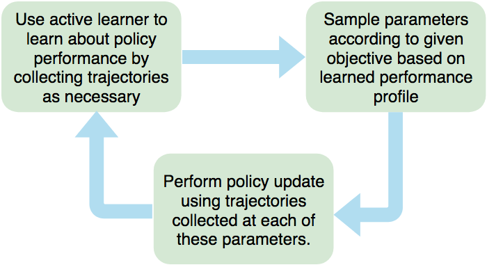
Figure 1. Main loop of the EffAcTS framework.

Active Learning is a paradigm where the agent chooses data to learn from based on its previous experience (see (Settles, 2009) for a comprehensive survey). It has been used to speedup learning tasks, especially in situations with limited data. An active learner not only needs to work with as few samples as possible, it also needs to account for the uncertainty in whatever data it has collected. These are exactly the desiderata of the required strategy, as it must be able to fit the performance function across $\mathbb{P}$ by collecting as few trajectories as possible, which come with noisy evaluations of the performance. Thus, quite clearly, the problem of efficiently performing such sampling is connected to active learning. The case of active learning that is of interest to us is when the agent is allowed to sample output for arbitrary points in the input space (instead of having to choose points from a finite dataset). The input here is some parameter $p$ from $\mathbb{P}$, and the output is the return from one trajectory collected at $p$.

We now outline our active learning framework for learning robust policies. Each policy update involves selectively generating trajectories to be sent to the batch policy optimization algorithm. This is done in two phases as follows:

Performance Assessment:

In the first phase, active learning is used to assess the performance of the current policy. To do this, an active learner sequentially picks some parameters and trajectories are sampled for each of them by setting the environment to these parameters and running the current policy. After a particular number of trials, it is in theory expected to have a reasonably good approximation of the performance as a function of the parameters, say $\hat{\eta}_{\theta_{i}}(p)$. Note that we have used $\theta_{i}$ as a subscript since this function is specific to the current policy with parameters $\theta_{i}$.

The active learner and this process are encapsulated in a subroutine LearnPerf that takes as input some policy parameters, $\theta$ and returns the function $\hat{\eta}_{\theta}$ as described above. LearnPerf could be equipped with persistent memory (e.g. to store data from previous iterations), and no assumptions are made about the form of the output $\hat{\eta}_{\theta}$ other than that it can be evaluated at any given $p\in\mathbb{P}$.

Parameter Selection:

The second phase uses this assessment to decide which parameters from $\mathbb{P}$ trajectories need to be collected for. This selection is guided by some given objective that enforces robustness. Another subroutine, SelectParams carries out this selection, taking as input a performance profile $\hat{\eta}_{\theta}$. Based on this performance profile, it returns a set $\mathbf{P}$ of parameters at which the policy needs to be trained.

The policy update is then performed using trajectories collected for each parameter in $\mathbf{P}$, and this is done for a given number ($N_{iters}$) of iterations. We call the resulting framework EffAcTS (Efficient Active Trajectory Sampling), and summarize it in Algorithm 1 and Figure 1. Any particular instantiation of EffAcTS is defined by the choice of active learning algorithm and also the scheme used to select which parts of $\mathbb{P}$ to sample from, i.e by specifying the LearnPerf and SelectParams subroutines.

1:for $i=0\ldots N_{iters}-1$ do

2:     $\hat{\eta}_{\theta_{i}}\leftarrow$ LearnPerf($\theta_{i}$)

3:     $\mathbf{P}\leftarrow$ SelectParams($\hat{\eta}_{\theta_{i}}$)

4:     $\boldsymbol{\tau}\leftarrow\left\{\right\}$

5:     for each $p\in\mathbf{P}$ do

6:         $\tau_{p}\leftarrow$ Trajectory collected at $p$ using $\pi_{\theta_{i}}$

7:         $\boldsymbol{\tau}\leftarrow\boldsymbol{\tau}\cup\tau_{p}$

8:     end for

9:     $\theta_{i+1}\leftarrow$BatchPolOpt($\boldsymbol{\tau}$, $\theta_{i}$)

10:end for

11:return $\theta_{N_{iters}}$

Algorithm 1 The EffAcTS framework

4.2. Applying EffAcTS

We analyze one such instantiation based on the CVaR objective for parameter selection. To generate samples of the bottom $\epsilon$ percentile of trajectories, a batch of parameters is sampled from $\mathcal{P}$, and trajectories are collected only for those that are in the worst $\epsilon$ percentile of performance according to $\hat{\eta}_{\theta}$. The use of Bandit algorithms for active learning is well studied in both Multi-Armed Bandit (Antos et al., 2008; Carpentier et al., 2011) as well as Linear Stochastic Bandit (Soare et al., 2013) settings. The parameter spaces involved in Robust RL are invariably continuous. LSBs and Gaussian Process Regression are two well-known approaches that can perform active regression on continuous spaces. LSBs, however, are specialized in the sense that they quickly seek out areas that lead to high reward, a property that we make use of as described shortly. Considering that Gaussian Processes are more computationally expensive, and also that LSBs are simpler to implement and can be very efficient, especially when data is scarce, we turn to LSBs as the active learner in our experiments.

Its arms are simply a large enough collection of parameters spread across $\mathbb{P}$. Pulling an arm $p\in\mathbb{P}$ results in a trajectory being sampled at $p$. Feedback is given to the bandit in an adversarial manner, being proportional to the negative of the return obtained on that sampled trajectory. This causes it to seek out regions with low performance, and in the process learn about the performance across $\mathcal{P}$. This behaviour is especially useful for identifying the worst-case parameters that are used in optimizing the CVaR objective.

We note that although the bandit’s learning phase is inherently serial, it is still possible to collect the trajectories for the estimated worst $\epsilon$ percentile of parameters in parallel.

We call this algorithm EffAcTS-C-B and its LearnPerf and SelectParams subroutines described in Algorithm 2. The following hyperparameters are introduced: $N_{B}$, the number of trajectories sampled by the bandit in the course of its learning, $N_{C}$, the total number of parameters chosen (this means that $\left\lceil\frac{N_{C}}{\epsilon}\right\rceil$ parameter values are drawn from the source distribution and their performance is estimated using the bandit, but only the bottom $N_{C}$ of those are used to collect trajectories). The most critical component is the LSB learner $B$ which incorporates internally a feature transformer $f$ that takes in a parameter from the source distribution’s support and applies some transformation on it (including possibly standardization), and also scales the negative returns given to it appropriately.

1:function LearnPerf($\theta$)

2:     for $i=1\ldots N_{B}$ do

3:         $p_{i}\leftarrow$ Optimal arm estimate by $B$.

4:         $\tau_{i}\leftarrow$ Trajectory collected at $p$ using $\pi_{\theta}$

5:         $R_{i}\leftarrow$ Return from $\tau_{i}$

6:         Update $B$ with $\left(p_{i},-R_{i}\right)$

7:     end for

8:     $\hat{\eta}_{\theta}\leftarrow$ Function parameterized by $B$’s current weights

9:     return $\hat{\eta}_{\theta}$

10:end function

1:function SelectParams($\hat{\eta}_{\theta}$)

2:     $\mathbf{P}\leftarrow\left\{\right\}$, $\hat{\mathbf{R}}\leftarrow\left\{\right\}$

3:     for  $j=1\ldots\left\lceil\frac{N_{C}}{\epsilon}\right\rceil$ do

4:         $p_{j}\leftarrow$ Parameter sampled from $\mathcal{P}$

5:         $\hat{R}_{j}\leftarrow$ $\hat{\eta}_{\theta}(p_{j})$

6:         Add $\hat{R}_{j}$ to $\hat{\mathbf{R}}$ and $p_{j}$ to $\mathbf{P}$

7:     end for

8:     $\mathbf{P}_{C}\leftarrow$ Subset of $\mathbf{P}$ giving rise to the bottom $\epsilon$ percentile of returns in $\hat{\mathbf{R}}$

9:     return $\mathbf{P}_{C}$

10:end function

Algorithm 2 Definitions of LearnPerf and SelectParams subroutines for EffAcTS-C-B

4.3. Sample Efficiency

Due to the fact that EffAcTS-C-B strategically chooses parameters at which to collect trajectories, we expect it to be able to maintain robustness and performance while collecting fewer samples than existing approaches. Consider for instance EPOpt(Rajeswaran et al., 2017), which discards a $1-\epsilon$ fraction of the trajectories it collects. If EPOpt collects $N$ trajectories, and EffAcTS-C-B’s bandit learner is allowed $N_{B}$ “arm pulls”, with the same number of trajectories being used for learning as EPOpt (i.e $N_{C}=\epsilon N$), the ratio of the total amount of data collected by the two algorithms is $\left(\frac{N_{B}+\epsilon N}{N}\right)$. For a nominal setting of $N=240$, $\epsilon=0.1$ and $N_{B}=24$, this results in a dramatic 80% reduction in the amount of data collected. We later show that efficiency gains of this order are indeed attainable in practice.

Parameter	$\mu$	$\sigma$	Low	High
Mass	6.0	1.5	3.0	9.0
Friction	2.0	0.25	1.5	2.5
Damping	2.5	2.0	1.0	4.0
Inertias	1.0	0.25	0.5	1.5

Parameter	$\mu$	$\sigma$	Low	High
Mass	6.0	1.5	3.0	9.0
Friction	0.5	0.1	0.3	0.7
Damping	1.5	0.5	0.5	2.5
Inertias	0.125	0.04	0.05	0.2

Table 1. Description of the source domain distribution for the Hopper (Left) and Half-Cheetah (Right) tasks. The values given here specify the means ($\mu$) and standard deviations ($\sigma$) for normal distributions truncated at the low and high points mentioned here. This is equivalent to the probability density of a normal distribution with parameters ($\mu,\sigma$) being zeroed outside the interval [Low, High], and being normalized so that it integrates to 1.

5. Connections to Multi-Task Learning

The problem of robust policy search on an ensemble of models can also be viewed as a form of transfer learning from simulated domains to an unseen real domain (possibly without any training on the real domain, which is referred to as direct-transfer or jumpstart (Taylor and Stone, 2009)). Further, the process of learning from an ensemble of models can be viewed as a Multi-Task Learning (MTL) problem with the set of tasks corresponding to the set of parameters that constitute the source domain distribution. Learning a robust policy corresponds to maintaining performance across this entire set of tasks, as is usually the goal in MTL settings. MTL, which is closely related to transfer learning, has been studied in the DRL context in a number of recent works (Rusu et al., 2016a; Rusu et al., 2016b; Parisotto et al., 2016; Sharma et al., 2018). However, these works consider only discrete and finite task sets, whereas model parameters form a (usually multi-dimensional) continuum. More generally, we can think of MTL with the task set being generated by a set of parameters, and refer to such problems as parameterized MTL problems, with Robust Policy Search being an instance of this setting.

(Sharma et al., 2018) has employed a bandit based active sampling approach similar to what we have described here to intelligently sample tasks (from a discrete and finite task set) to train on for each iteration. The feedback to the bandit is also given in an adversarial manner. However, we note several differences when it comes to a parameterized MTL setting. The first is the functional dependence of the task performance to an underlying parameter as discussed earlier. In the discrete MTL settings usually studied (such as Atari Game playing tasks), there is no such visible dependency that can be modeled. This means that any algorithm that is adapted to the parameterized setting need to be reworked to utilize such dependencies as EffAcTS does. The task selection procedure in EffAcTS differs from the one in (Sharma et al., 2018) in that the performance is sampled for several tasks in between iterations of policy training. Additionally, one single task is not chosen in the end, rather the active learner is used to inform the selection of a group of tasks as necessary for the given objective.

6. Experiments

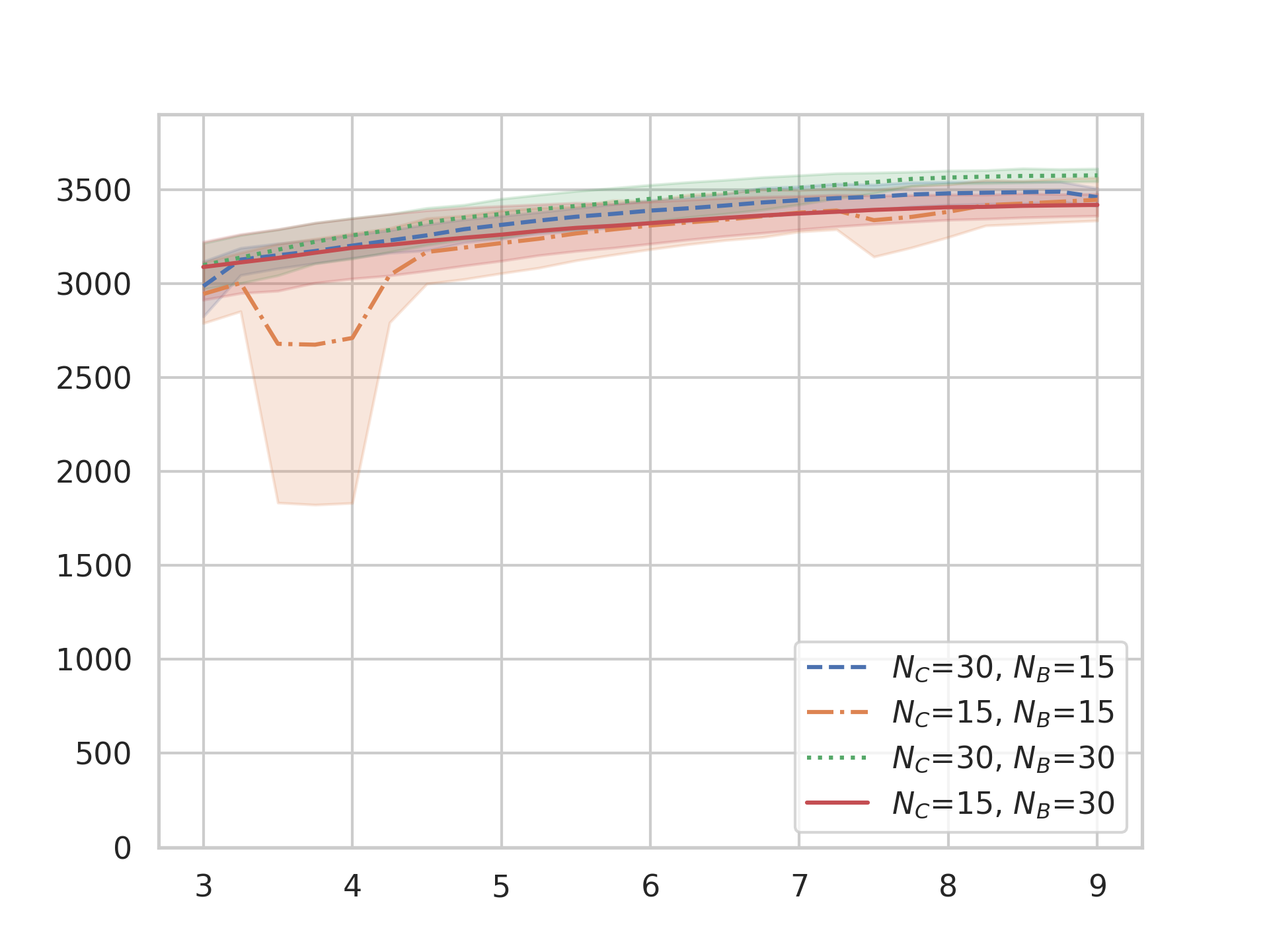
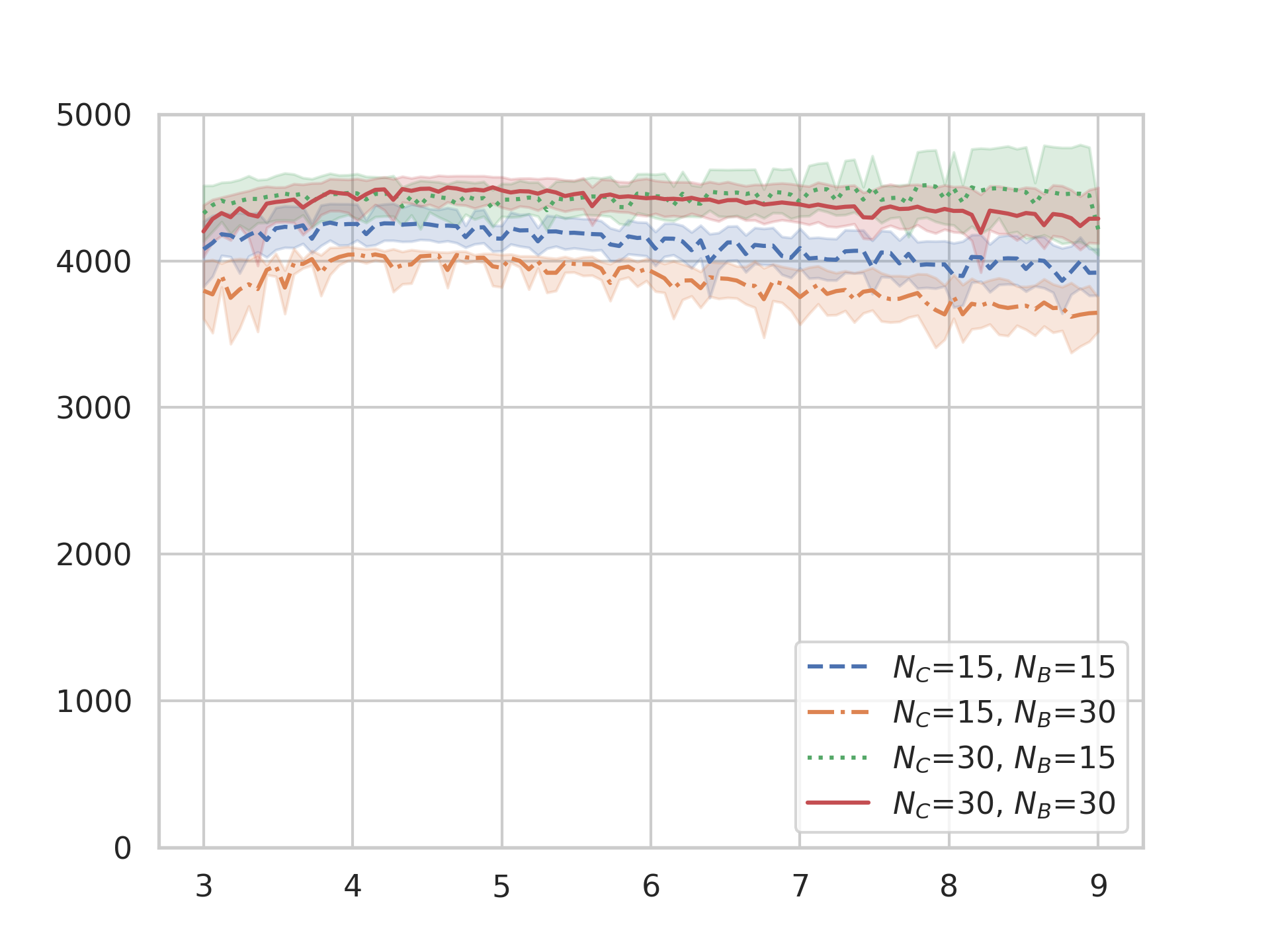
Figure 2. Performance (y-axis) as a function of torso mass (x-axis) for $\epsilon=0.1$ for the Hopper (Left) and Half-Cheetah (Right) tasks. The bands indicate the confidence intervals of the performance measured across 5 runs of the entire training procedure. All of the configurations tested use at least 75% fewer trajectories than EPOpt, and with the exception of $N_{C}=15$ and $N_{B}=15$ in the Hopper task alone, perform to the same extent and are as robust as EPOpt (acccording to results reported in (Rajeswaran et al., 2017)).

As EPOpt(Rajeswaran et al., 2017) uses the CVaR objective, it is a very suitable baseline against which to compare EffAcTS-C-B for demonstrating the benefits of introducing the active learner. We conduct experiments to answer the following questions, which we will reference as RQ1, RQ2 etc. in later discussions:

1. Do the policies learned using EffAcTS-C-B suffer any degradation in performance from that of EPOpt? Is robustness preserved across the same range of model parameters as in EPOpt?

2. Does the bandit active sampler identify with reasonable accuracy the region corresponding to the worst $\epsilon$ percentile of performance, and does it achieve a reasonable fit to the performance across the range of parameters (i.e has it explored enough to avoid errors due to the noisy evaluations it receives)?

3. How much can the sample efficiency be improved upon? This mainly boils down to asking how few trajectories are sufficient for the bandit to learn well enough.

6.1. Implementation Details and Hyperparameters

The experiments are performed on the standard Hopper and Half-Cheetah continuous control tasks available in OpenAI Gym (Brockman et al., 2016), simulated with the MuJoCo Physics simulator (Todorov et al., 2012). As in (Rajeswaran et al., 2017), some subset of the following parameters of the robot can be varied: Torso Mass, Friction with the ground, Foot Joint Damping and Joint Inertias. We also use the same statistics for the source distributions of the parameters which are described in Table 1.

We emphasize that because we are using the same environments in (Rajeswaran et al., 2017) and also the same policy parameterization, results reported there can be used directly to compare against EffAcTS-C-B.

Hyperparameters	Median %tile	Avg %tile	Std. Dev.	Max %tile
$N_{C}$=15, $N_{B}$=15	14.6	15.9	7.7	32.2
$N_{C}$=15, $N_{B}$=30	14.9	23.4	24.0	98.0
$N_{C}$=30, $N_{B}$=15	13.7	23.0	19.4	74.7
$N_{C}$=30, $N_{B}$=30	11.6	14.9	10.6	47.8

Table 2. Statistics for the percentiles described in section 6.6 for the Hopper task’s 1-D model ensemble with $\epsilon=0.1$, which are measured every fifth iteration from the 100th to the 150th iterations.

We use the hyperparameter settings for TRPO suggested in OpenAI Baselines (Dhariwal et al., 2017) on which our implementation is also based. These are shown in Table 3.

Hyperparameter	Value
Timesteps per batch	1024
Max KL	0.01
CG Iters	10
CG Damping	0.1
$\gamma$	0.99
$\lambda$	0.98
VF Iterations	5
VF Stepsize	1e-3

Table 3. Hyperparameters for TRPO

One difference from EPOpt’s implementation is that we use Generalized Advantage Estimation (Schulman et al., 2016) instead of subtracting a baseline from the value function. For value function estimation using a critic, we use the same NN architecture as the policy, 2 hidden layers of 64 units each. Policies are parameterized with NNs and have two hidden layers with 64 units each, and use $\tanh$ as the activation function.

6.2. Bandit Algorithm

For all our experiments, we implement the bandit learner using Thompson Sampling due to its simplicity, following the version described in (Abeille and Lazaric, 2017). The hyperparameters introduced by this are as in Table 4 (they have the same names as in the paper).

Hyperparameter	Value
$R$	5.0
$\delta$	0.1
$\lambda$	0.5

Table 4. Thompson Sampling Hyperparameters

The first two parameters control the amount of exploration performed during Thompson Sampling, while $\lambda$ is a regularization parameter for the parameter estimates.

The arms of the bandit are model parameters taken uniformly across the domain and converted to feature values. In order to allow for some degree of expressiveness for the fit, we apply polynomial transformations of some particular degree to the model parameters. The features input to the bandit are 4th degree polynomial terms generated from the model parameters. This amounts to 5 terms in the 1-D case and 15 in the 2-D case. These arm “representations” are then standardized before being used by the bandit. The negative returns given as feedback to the bandit are scaled by a factor of $10^{-3}$.

6.3. (RQ1) Performance and Robustness

In this section, we perform the following experiment to evaluate EffAcTS-C-B for the objectives of RQ1. In this experiment, only one environment parameter (torso mass) is varied, creating a 1-D model ensemble on which to evaluate the algorithm.

The torso mass is varied in both the Hopper and the Half-Cheetah domains keeping the rest of the parameters fixed at their mean values. The performance of the EffAcTS-C-B learned policy is then tested across this range, and the results are shown in Figure 2. We use Trust Region Policy Optimization (TRPO) (Schulman et al., 2015) for batch policy optimization and run it for 150 iterations. For this part, we use 4th degree polynomial transformations.

We see that the policy is indeed robust as it maintains its performance across the range of values of the torso mass, and it achieves near or better than the best performance for both tasks as reported in (Rajeswaran et al., 2017) in all but one case, with $N_{C}=15$ and $N_{B}=15$ for Hopper. This setting samples the least number of trajectories per iteration, 30, which is just one eighth of the 240 drawn in EPOpt. Although there is one region where it is unstable, it is still able to maintain its performance everywhere else, thus attaining the same level of robustnes as EPOpt. Further, the performance achieved is almost as good as, and possibly better than EPOpt(Rajeswaran et al., 2017).

For the other settings which use more trajectories, this does not happen, and even at $N_{C}=30$ and $N_{B}=30$ which samples the most trajectories, a 75% reduction in samples collected is achieved over EPOpt (the total number of iterations is the same). The other two settings which perform almost as well in both tasks collect 45 each, which amounts to an even larger reduction of 81.2%. In the case of $N_{C}=15$ and $N_{B}=15$ with the Half-Cheetah Task, this number is pushed even further to 87.5% while still retaining performance and robustness.

6.4. (RQ1) Performance on a 2-D Model Ensemble

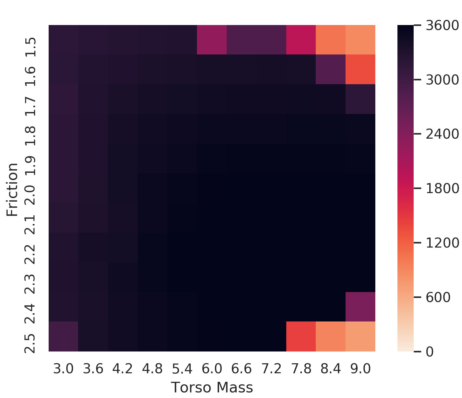
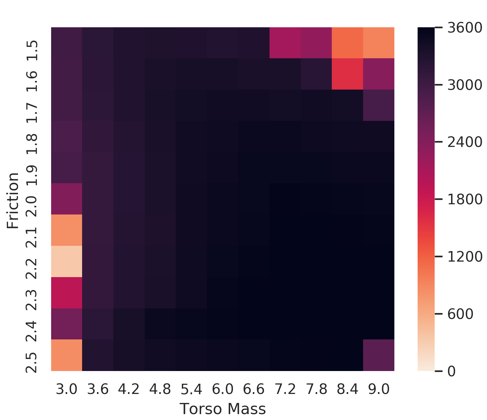
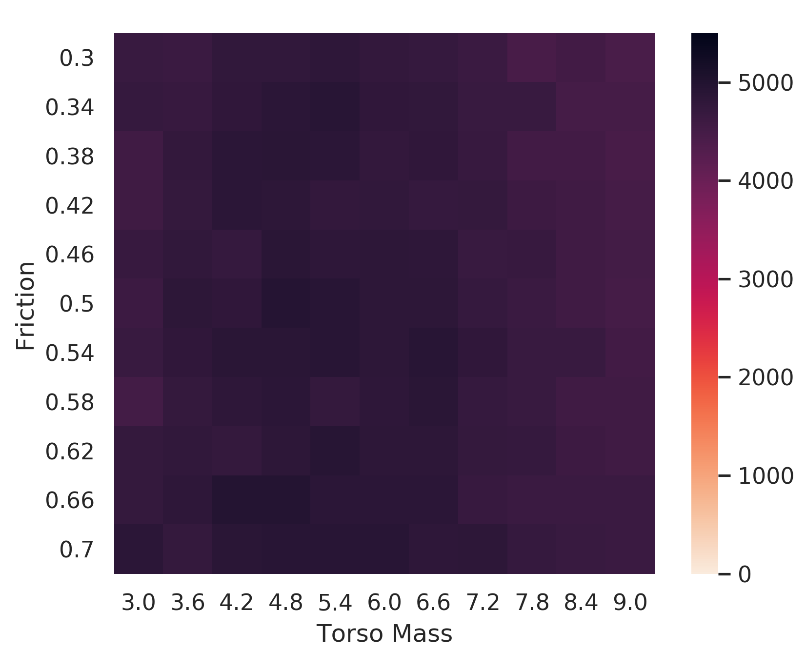
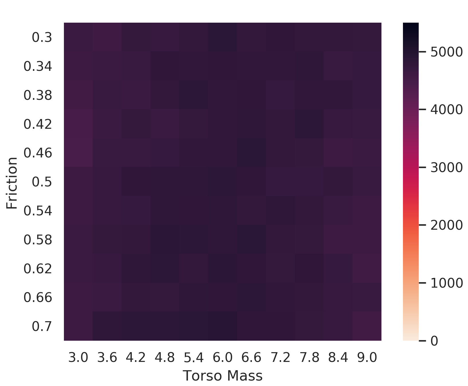
Figure 3. Performance as a function of torso mass and ground friction on the Hopper (left half) and Half-Cheetah (right half) tasks for $\epsilon=0.1$ for one run or EffAcTS-C-B. In each row, Left: $N_{C}$=30, $N_{B}$=30. Right: $N_{C}$=30, $N_{B}$=50.

In this question, we further investigate the scalability of the algorithm to larger model ensembles, again in the context of RQ1. In this experiment, we vary the friction with the ground in addition to the torso mass, thus creating a two dimensional ensemble of parameters. Here, we run TRPO for 200 iterations, and again use 4th degree polynomial transformations. Figure 3 shows the results obtained.

Full performance is maintained over almost all of the parameter space in both domains, again being comparable to or better than in (Rajeswaran et al., 2017). Notably, with $N_{C}$=30, $N_{B}$=30, the same 75% reduction in collected trajectories is obtained even in a higher dimensional model ensemble. This is also despite the added challenge of an increased number of parameters for the bandit to fit (15 as opposed to 5 in the previous experiment).

6.5. Visualizing the Bandit Active Learner

In Figure 4, we present the outcome from one particular iteration of training. The true performance profile is estimated by collecting 100 trajectories to calculate the mean return at each parameter (again, these trajectories are not used for learning). Along with this is shown the bandit’s fit, the trajectories it collects while learning and the trajectories that are sampled based on its estimate of the bottom $\epsilon=0.1$ percentile (output used for training the policy).

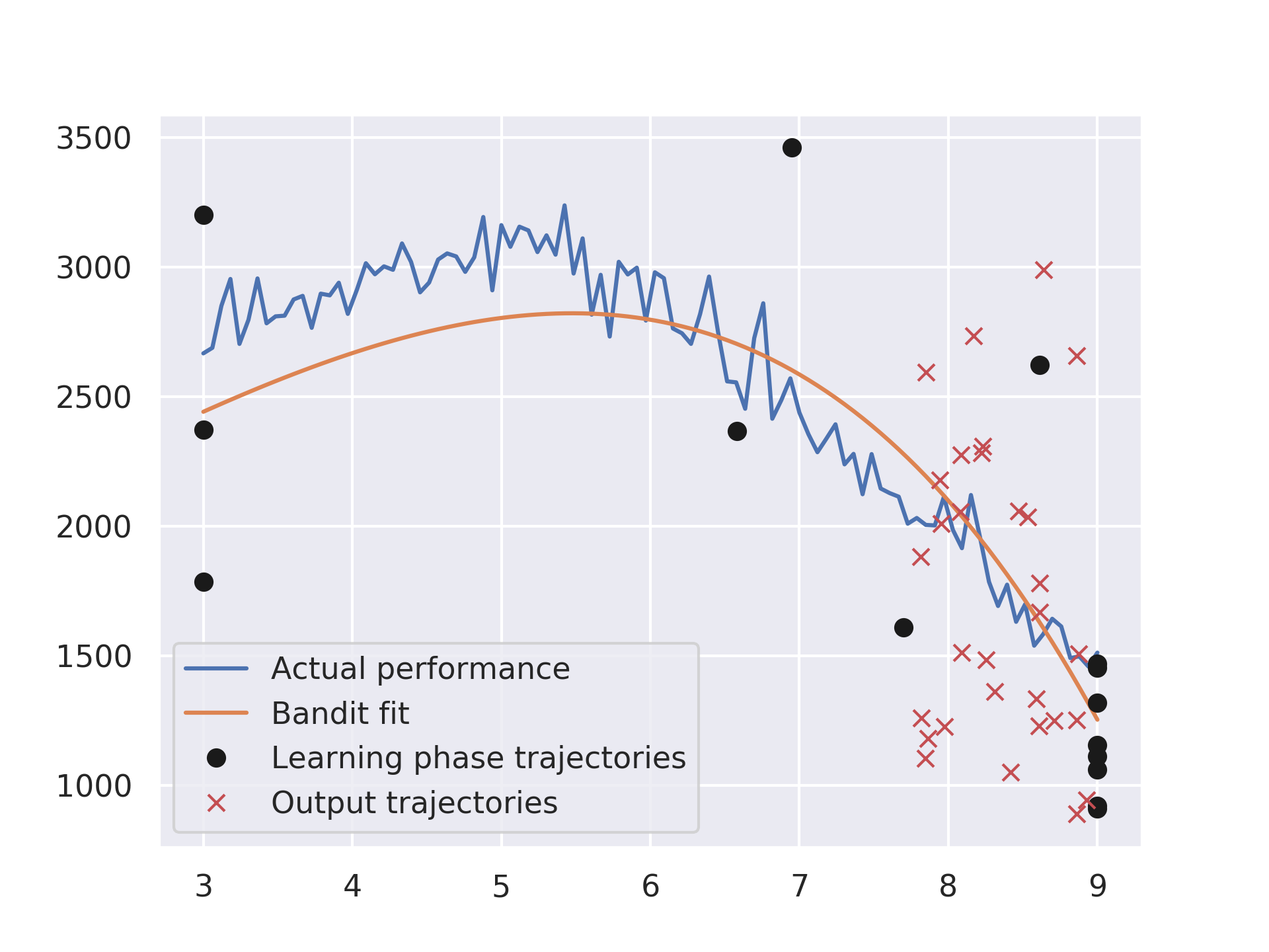
Figure 4. The bandit’s operation in the 115th iteration of training in the Hopper task. Individual trajectories are shown as dots or crosses, with the position indicating the parameter value and the return obtained.

We see that the bandit takes exploratory actions (points to the left and in the middle) that don’t lead to the worst returns. However, it quickly moves towards the region with low returns, and the final fit is close to the true mean performance. From comparison with the output trajectories, the trajectories in the learning phase are quite clearly not representative of the bottom $\epsilon=0.1$ percentile according to the source distribution. Thus, we cannot reuse these to perform learning with the CVaR objective.

We also note that a perfectly learned performance profile is not necessary to sample from the worst trajectories. As long as the fit is reasonably accurate in that region, the output trajectories will be of good quality. In practice, we expect LSB algorithms to be capable of doing this as they tend to focus on these regions.

6.6. (RQ2) Analysis of the Bandit Active Learner

Here we validate one of our key assumptions, that the active learner learns well enough about the performance that it can produce a decent approximation of a sample batch of the bottom $\epsilon$ percentile of trajectories. For this, we first evaluate the average return for a batch of samples from $\mathcal{P}$ by collecting a large number of trajectories at each parameter. We note that these trajectories are solely for the purpose of analysis and are not used to perform any learning. Then, the percentile of the trajectory deemed to have the greatest return among those chosen based on the bandit learner is computed using the returns in this batch by using a nearest-neighbor approximation. This is done across several iterations during the training, and the median percentiles along with other statistics are reported in Table 2 for the Hopper task.

Ideally, we would like this value to come out to around $100\epsilon$ (when written as proper percentiles), i.e the parameter with the greatest performance among the worst $\epsilon$ percentile should be at the $\epsilon^{th}$ percentile. In our estimates, there are some outliers that cause the average to become large, but as the median value shows, it is indeed reasonably close to the desired value of 10 for $\epsilon=0.1$.

6.7. (RQ3) Non-stationary Bandits for Data Reuse

In this section, we attempt to answer RQ3 by considering modifications that can be made to EffAcTS-C-B, so that it uses lesser data, while also achieving a level of performance and robustness that is close to the results above.

Particularly, we investigate the use of a modified version of the Thompson Sampling algorithm above that is suited for non-stationary scenarios. This is done in order to reuse performance history from previous iterations to estimate the bandit’s parameters with the aim of achieving a further reduction in sample complexity. To implement this, past data is weighted down in the Linear Regression step of Thompson Sampling, and the weight decays after each iteration by a factor $\alpha$. That is, at the $i^{th}$ iteration, the data from the $i^{th}$, $\left(i-1\right)^{th}$$\ldots$$\left(i-k\right)^{th}$ iterations would have weights 1, $\alpha$$\ldots$$\alpha^{k}$ respectively.

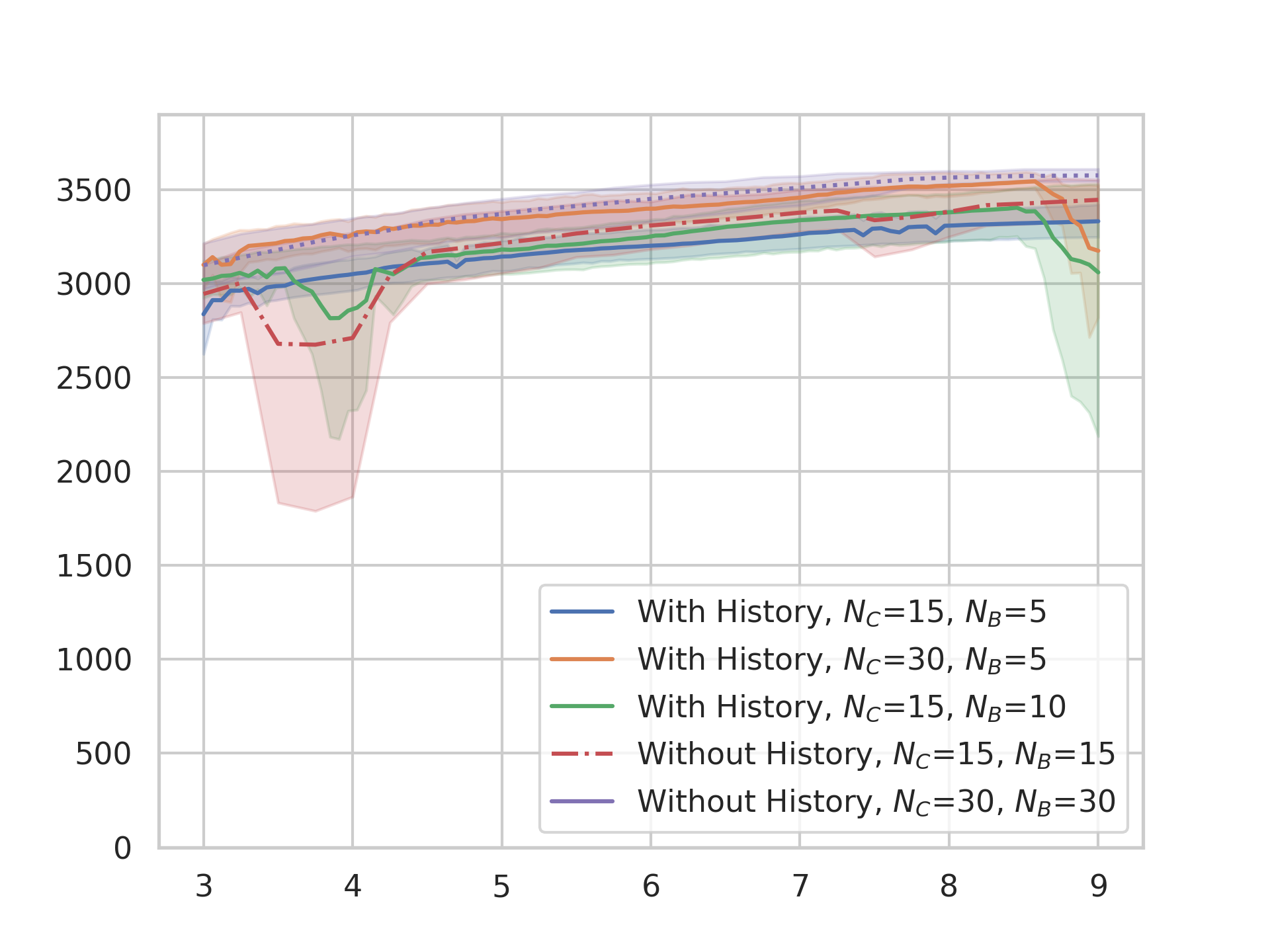
Figure 5. Results (performance vs. torso mass) for the non-stationary-bandit version (labeled “With history”) of EffAcTS-C-B, along with the original EffAcTS-C-B results (labeled “Without history”) on the Hopper 1-D ensemble. A value of $\alpha=0.25$ was used, with the other hyperparameters remaining unchanged. As before, the plot shows the performance as a function of torso mass for $\epsilon=0.1$, and the bands indicate the confidence intervals of the performance measured across 5 runs of the entire training procedure. This time, with 92% fewer trajectories than EPOpt, the configuration $N_{C}=15$, $N_{B}=5$ with history is able to perform comparably to EPOpt, as well as EffAcTS without history and using more trajectories.

We compare this version with the original setup in Figure 5. We see that the setting with the smallest number of trajectories collected with history ($N_{C}=15$, $N_{B}=5$) is more robust than the vanilla case with $N_{C}=15$, $N_{B}=15$ and performs nearly as well (despite cutting down on 10 more trajectories). With more data, some loss of robustness is encountered, but the performance improves, and becomes comparable to the best original case ($N_{C}=30$, $N_{B}=30$).

6.8. Other Remarks

We note that we do not perform “pre-training” as in EPOpt where the entire batch of trajectories is used for policy learning for some iterations at the beginning (corresponding to optimizing for the average return over the ensemble). This has been reported to be necessary, possibly due to problems with initial exploration if using the CVaR objective from the beginning. EffAcTS-C-B on the other hand works without any such step. However, at the very beginning, we collect trajectories for parameters sampled directly from $\mathcal{P}$ until 2048 time steps have elapsed in that iteration. This is because algorithms like TRPO have been known to require at least that much data per iteration.

7. Conclusions and Further Possibilities

We developed the EffAcTS framework for using active learning to make an informed selection of model parameters based on agent performance, which can subsequently be used to judiciously generate trajectories for robust RL. With an illustration of this framework based on Linear Bandits and the CVaR objective, we have both demonstrated its applicability for robust policy search as well as established its effectiveness in reducing sample complexity by way of empirical evaluations on standard continuous control domains. We also discussed our work in the context of Multi-Task Learning along with the similarities and differences between these settings.

Our work opens up requirements for active learning algorithms that can work well with even lesser data than we need here. Methods like Gaussian Process Regression are known to be efficient, but not in high dimensional spaces. For robust policy search methods to be effective for transfer from simulation to reality, they need to be able to handle the complexities of the real world, which necessitates methods that work with high dimensional model ensembles, which in turn entail frameworks such as EffAcTS to help reduce the sample complexity. Another possibility for robust policy search itself is to develop objectives that can speedup learning as well as make use of the features of EffAcTS to maintain sample efficiency.

With our interpretation of robust policy search as a parameterized version of Multi-Task Learning, a natural next step would be to adapt developments in the usual discrete MTL setting to robust policy search. It would also be worthwhile to similarly investigate the applicability of Meta Learning, as it would prove useful for both dealing with large disparities between the source domains and the real world, as well as coping with unmodeled dynamics (which are unavoidable since it is not feasible to model the real world with complete accuracy).

8. Acknowledgments

The authors thank the Robert Bosch Center for Data Science and AI, IIT Madras for funding this work and providing the requisite computing resources. We also thank Aravind Rajeswaran for valuable pointers and suggestions, and OpenAI for their excellent codebase of Deep RL algorithms.

References

- (1)
- Abbasi-Yadkori et al. (2011) Yasin Abbasi-Yadkori, Dávid Pál, and Csaba Szepesvári. 2011. Improved Algorithms for Linear Stochastic Bandits. In Proceedings of the 24th International Conference on Neural Information Processing Systems.
- Abeille and Lazaric (2017) Marc Abeille and Alessandro Lazaric. 2017. Linear Thompson Sampling Revisited. In Proceedings of the 20th International Conference on Artificial Intelligence and Statistics.
- Agrawal and Goyal (2013) Shipra Agrawal and Navin Goyal. 2013. Thompson Sampling for Contextual Bandits with Linear Payoffs. In Proceedings of the 30th International Conference on International Conference on Machine Learning - Volume 28.
- Antos et al. (2008) András Antos, Varun Grover, and Csaba Szepesvári. 2008. Active Learning in Multi-armed Bandits. In Proceedings of the 19th International Conference on Algorithmic Learning Theory.
- Brockman et al. (2016) Greg Brockman, Vicki Cheung, Ludwig Pettersson, Jonas Schneider, John Schulman, Jie Tang, and Wojciech Zaremba. 2016. OpenAI Gym. arXiv:arXiv:1606.01540
- Carpentier et al. (2011) Alexandra Carpentier, Alessandro Lazaric, Mohammad Ghavamzadeh, Rémi Munos, and Peter Auer. 2011. Upper-Confidence-Bound Algorithms for Active Learning in Multi-armed Bandits. In Algorithmic Learning Theory. Springer Berlin Heidelberg.
- Dhariwal et al. (2017) Prafulla Dhariwal, Christopher Hesse, Oleg Klimov, Alex Nichol, Matthias Plappert, Alec Radford, John Schulman, Szymon Sidor, Yuhuai Wu, and Peter Zhokhov. 2017. OpenAI Baselines. https://github.com/openai/baselines.
- Hiraoka et al. (2019) Takuya Hiraoka, Takahisa Imagawa, Tatsuya Mori, Takashi Onishi, and Yoshimasa Tsuruoka. 2019. Learning Robust Options by Conditional Value at Risk Optimization. In NeurIPS. 2615–2625. http://papers.nips.cc/paper/8530-learning-robust-options-by-conditional-value-at-risk-optimization
- Kurutach et al. (2018) Thanard Kurutach, Ignasi Clavera, Yan Duan, Aviv Tamar, and Pieter Abbeel. 2018. Model-Ensemble Trust-Region Policy Optimization. In ICLR.
- Lee et al. (2019) Gilwoo Lee, Brian Hou, Aditya Mandalika, Jeongseok Lee, and Siddhartha S. Srinivasa. 2019. Bayesian Policy Optimization for Model Uncertainty. In ICLR. https://openreview.net/forum?id=SJGvns0qK7
- Li et al. (2010) Lihong Li, Wei Chu, John Langford, and Robert E. Schapire. 2010. A Contextual-bandit Approach to Personalized News Article Recommendation. In Proceedings of the 19th International Conference on World Wide Web.
- Lillicrap et al. (2016) Timothy P. Lillicrap, Jonathan J. Hunt, Alexander Pritzel, Nicolas Heess, Tom Erez, Yuval Tassa, David Silver, and Daan Wierstra. 2016. Continuous control with deep reinforcement learning. In ICLR.
- Mordatch et al. (2015) I. Mordatch, K. Lowrey, and E. Todorov. 2015. Ensemble-CIO: Full-body dynamic motion planning that transfers to physical humanoids. In 2015 IEEE/RSJ International Conference on Intelligent Robots and Systems (IROS).
- Morimoto and Doya (2001) Jun Morimoto and Kenji Doya. 2001. Robust Reinforcement Learning. In Advances in Neural Information Processing Systems 13.
- Parisotto et al. (2016) Emilio Parisotto, Jimmy Ba, and Ruslan Salakhutdinov. 2016. Actor-Mimic: Deep Multitask and Transfer Reinforcement Learning. In ICLR.
- Peng et al. (2018) X. B. Peng, M. Andrychowicz, W. Zaremba, and P. Abbeel. 2018. Sim-to-Real Transfer of Robotic Control with Dynamics Randomization. In 2018 IEEE International Conference on Robotics and Automation (ICRA).
- Pinto et al. ([n.d.]) Lerrel Pinto, James Davidson, Rahul Sukthankar, and Abhinav Gupta. [n.d.]. Robust Adversarial Reinforcement Learning. In Proceedings of the 34th International Conference on Machine Learning. PMLR.
- Rajeswaran et al. (2017) Aravind Rajeswaran, Sarvjeet Ghotra, Balaraman Ravindran, and Sergey Levine. 2017. EPOpt: Learning Robust Neural Network Policies Using Model Ensembles. In International Conference on Learning Representations.
- Ramos et al. (2019) Fabio Ramos, Rafael Possas, and Dieter Fox. 2019. BayesSim: adaptive domain randomization via probabilistic inference for robotics simulators. In Robotics: Science and Systems (RSS). https://arxiv.org/abs/1906.01728
- Rusu et al. (2016a) Andrei A. Rusu, Sergio Gomez Colmenarejo, Caglar Gulcehre, Guillaume Desjardins, James Kirkpatrick, Razvan Pascanu, Volodymyr Mnih, Koray Kavukcuoglu, and Raia Hadsell. 2016a. Policy distillation. In ICLR.
- Rusu et al. (2016b) Andrei A. Rusu, Neil C. Rabinowitz, Guillaume Desjardins, Hubert Soyer, James Kirkpatrick, Koray Kavukcuoglu, Razvan Pascanu, and Raia Hadsell. 2016b. Progressive Neural Networks. CoRR abs/1606.04671 (2016).
- Schulman et al. (2015) John Schulman, Sergey Levine, Philipp Moritz, Michael Jordan, and Pieter Abbeel. 2015. Trust Region Policy Optimization. In Proceedings of the 32Nd International Conference on International Conference on Machine Learning - Volume 37.
- Schulman et al. (2016) John Schulman, Philipp Moritz, Sergey Levine, Michael Jordan, and Pieter Abbeel. 2016. High-Dimensional Continuous Control Using Generalized Advantage Estimation. In Proceedings of the International Conference on Learning Representations (ICLR).
- Schulman et al. (2017) John Schulman, Filip Wolski, Prafulla Dhariwal, Alec Radford, and Oleg Klimov. 2017. Proximal Policy Optimization Algorithms. CoRR abs/1707.06347 (2017).
- Settles (2009) B. Settles. 2009. Active Learning Literature Survey. Computer Sciences Technical Report 1648. University of Wisconsin–Madison.
- Sharma et al. (2018) Sahil Sharma, Ashutosh Kumar Jha, Parikshit S Hegde, and Balaraman Ravindran. 2018. Learning to Multi-Task by Active Sampling. In International Conference on Learning Representations.
- Soare et al. (2013) Marta Soare, Alessandro Lazaric, and Remi Munos. 2013. Active Learning in Linear Stochastic Bandits. In NIPS 2013 Workshop on Bayesian Optimization in Theory and Practice.
- Tamar et al. (2015) Aviv Tamar, Yonatan Glassner, and Shie Mannor. 2015. Optimizing the CVaR via Sampling. In AAAI.
- Taylor and Stone (2009) Matthew E. Taylor and Peter Stone. 2009. Transfer Learning for Reinforcement Learning Domains: A Survey. J. Mach. Learn. Res. (2009).
- Tobin et al. (2017) Josh Tobin, Rachel Fong, Alex Ray, Jonas Schneider, Wojciech Zaremba, and Pieter Abbeel. 2017. Domain randomization for transferring deep neural networks from simulation to the real world. In IROS. IEEE, 23–30.
- Todorov et al. (2012) E. Todorov, T. Erez, and Y. Tassa. 2012. MuJoCo: A physics engine for model-based control. In 2012 IEEE/RSJ International Conference on Intelligent Robots and Systems.
- Wang et al. (2010) Jack M. Wang, David J. Fleet, and Aaron Hertzmann. 2010. Optimizing Walking Controllers for Uncertain Inputs and Environments. In ACM SIGGRAPH 2010 Papers.
- Wang et al. (2017) Ziyu Wang, Victor Bapst, Nicolas Heess, Volodymyr Mnih, Remi Munos, Koray Kavukcuoglu, and Nando de Freitas. 2017. Sample Efficient Actor-Critic with Experience Replay. In ICLR.
- Yu et al. (2017) Wenhao Yu, Jie Tan, Karen Liu, and Greg Turk. 2017. Preparing for the Unknown: Learning a Universal Policy with Online System Identification. In Robotics: Science and Systems (RSS).