Symmetric integrators based on continuous-stage Runge-Kutta-Nyström methods for reversible systems

Abstract

In this paper, we study symmetric integrators for solving second-order ordinary differential equations on the basis of the notion of continuous-stage Runge-Kutta-Nyström methods. The construction of such methods heavily relies on the Legendre expansion technique in conjunction with the symmetric conditions and simplifying assumptions for order conditions. New families of symmetric integrators as illustrative examples are presented. For comparing the numerical behaviors of the presented methods, some numerical experiments are also reported.

1 Introduction

Numerical integration that preserves at least one of geometric properties of a given dynamical system has attracted much attention in these years [13, 15, 24]. As suggested by Kang Feng [11, 13], it is natural to look forward to those discrete systems which preserve as much as possible the intrinsic properties of the continuous system — this is a truly ingenious idea for devising “good” integrators to properly simulate the evolution of various dynamical systems with geometric features. It is evidenced that numerical methods with such a special purpose can not only perform a more accurate long-time integration than those traditional methods without any geometric-feature preservation, but also produce an improved qualitative behavior [15]. Such type of methods, generally associated with the terminology “geometric integration”, are distinguished by the geometric properties they inherit, including symplectic methods for Hamiltonian systems, symmetric methods for reversible systems, volume-preserving methods for divergence-free systems, invariant-preserving methods for conservative systems, multi-symplectic methods for Hamiltonian partial differential equations etc. For more details, we refer the interested readers to [11, 13, 15, 24, 17] and references therein.

Reversible systems and reversible maps are of interest in both aspects of theoretical study and numerical simulation for many differential equations [15]. Let $\rho$ be an invertible linear transformation in the phase space of a first-order system given by $z^{\prime}=f(z)$, then the system is called $\rho$-reversible if [15]

$$\rho f(z)=-f(\rho z),\,\text{for}\;\forall\,z,$$

and a map $\phi(z)$ is called $\rho$-reversible if

$$\rho\circ\phi=\phi^{-1}\circ\rho.$$

Particularly, it is shown in [15] that all second-order systems with the form $z^{\prime\prime}=f(z)$ are reversible as they can be transformed into reversible first-order systems. In addition, notice that the exact flow of a reversible system is a reversible map, it is therefore natural to find a numerical method $\Phi_{h}$, which is better referred to as a reversibility-preserving integrator, such that it is also a reversible map (i.e., $\rho\circ\Phi_{h}=\Phi_{h}^{-1}\circ\rho$). It is known that a number of symmetric integrators automatically possess this property, e.g., all symmetric Runge-Kutta (RK) methods, some partitioned Runge-Kutta (PRK) methods for special partitioned systems, some composition and splitting methods, and standard projection methods for differential equations on special manifolds (see [15], page 145). To be specific, we quote the following result from [25].

Theorem 1.1.

[25] A Runge-Kutta method or a Runge-Kutta-Nyström (RKN) method is reversible iff it is symmetric.

Thanks to the property of reversibility preservation, symmetric integrators often have an excellent long-time numerical behavior than those non-symmetric integrators for reversible systems [15]. So far, a wide variety of effective symmetric integrators have been proposed (see [6, 7, 9, 13, 15, 19, 25] and references therein).

In the context of geometric integration, the greatest interest has been given to the development of symplectic integrators for solving Hamiltonian systems over the last decades [13, 15, 24]. However, if the Hamiltonian $H(p,q)$ satisfies $H(-p,q)=H(p,q)$, then the system is reversible with respect to the linear transformation $\rho:(p,q)\mapsto(-p,q)$. Particularly, a well-known class of separable Hamiltonian systems determined by the Hamiltonian $H(p,q)=\frac{1}{2}p^{T}Mp+U(q)$ happens to be such type of reversible systems. Therefore, it makes sense for devising a numerical method that preserves symplecticity and reversibility at the same time, and fortunately, this has been shown to be an attainable goal (see [6, 13, 14, 15, 22, 26, 28] and references therein). Besides, a numerical method which is energy-preserving and reversibility-preserving can also be of interest [1, 2, 3, 4, 5, 16, 23, 26, 28].

In recent years, numerical methods with infinitely many stages including continuous-stage Runge-Kutta (csRK) methods, continuous-stage partitioned Runge-Kutta (csPRK) methods and continuous-stage Runge-Kutta-Nyström (csRKN) methods are presented and discussed by several authors, see [1, 16, 18, 20, 21, 26, 27, 28, 29, 31, 32, 33, 34, 35]. They can be viewed as the natural generalizations of numerical methods with finite stages (e.g., classical RK methods). It is shown in [28, 29, 31, 32, 33, 34, 35] that by using continuous-stage methods many classical RK, PRK and RKN methods of arbitrary order can be derived, without resort to solving the tedious nonlinear algebraic equations (associated with order conditions) in terms of many unknown coefficients. The construction of continuous-stage methods seems much easier than that of those traditional methods with finite stages, as the associated Butcher coefficients are “continuous” or “smooth” functions and hence they can be treated by using some analytical tools [28, 29, 31, 32, 33, 34, 35]. Moreover, as presented in [4, 16, 18, 20, 21, 28, 29, 31, 32, 33, 34, 35], numerical methods serving some special purpose including symplecticity-preserving methods for Hamiltonian systems, symmetric methods for reversible systems, energy-preserving methods for conservative systems can also be established within this new framework. Besides, a well known negative result we have to mention here is that no RK methods is energy-preserving for general non-polynomial Hamiltonian systems [8], in contrast to this, energy-preserving csRK methods can be easily constructed [1, 2, 16, 18, 23, 26, 27, 28, 20]. In addition, as presented in [27, 30], some Galerkin variational methods can be interpreted as continuous-stage (P)RK methods, but they can not be completely understood in the classical (P)RK framework. Therefore, continuous-stage methods have granted us a new insight for numerical integration of differential equations and some subjects in this new area need to be investigated.

Since symmetric integrators possess important theoretical and real values in numerical ordinary differential equations [7, 15, 19, 25], we are concerned with the development of new symmetric integrators for solving second-order ordinary differential equations (ODEs). The construction of such methods in this paper is on the basis of the notion of csRKN methods and heavily relies on the Legendre polynomial expansion technique. Furthermore, by using Gaussian and Lobatto quadrature formulas we show that new families of symmetric RKN-type schemes can be easily devised. Moreover, by Theorem 1.1, these methods are also reversibility-preserving and therefore very suitable for solving reversible systems.

This paper will be organized as follows. In Section 2, we introduce the exact definition of csRKN methods for solving second-order ODEs and the corresponding order theory previously developed in [32] will be briefly revisited. In Section 3, by using Legendre expansion technique, we present some useful results for devising symmetric integrators which is then followed by giving some illustrative examples for deriving new symmetric integrators in Section 4. Some numerical experiments are reported in section 5. At last, we give some concluding remarks in Section 6 to end this paper.

2 Continuous-stage RKN method and its order theory

In this section, we will recall the notion of the so-called continuous-stage Runge-Kutta-Nyström (csRKN) methods and review some known results which are useful for constructing such methods of arbitrarily high order. For more details, see [31, 32].

2.1 Continuous-stage RKN method

Consider the following initial value problem governed by a second-order system

$$q^{\prime\prime}=f(t,q),\;q(t_{0})=q_{0},\,q^{\prime}(t_{0})=q^{\prime}_{0},$$ (2.1)

where $f:\mathbb{R}\times\mathbb{R}^{d}\rightarrow\mathbb{R}^{d}$ is a smooth vector-valued function.

A well-known numerical method for solving (2.1) is the so-called RKN method with $s$ stages, which can be depicted as

$$Q_{i} =q_{0}+hc_{i}q^{\prime}_{0}+h^{2}\sum\limits_{j=1}^{s}\bar{a}_{ij}f(t_{0}+c_{j}h,Q_{j}),\;i=1,\cdots,s,$$ (2.2a)

$$q_{1} =q_{0}+hq^{\prime}_{0}+h^{2}\sum\limits_{i=1}^{s}\bar{b}_{i}f(t_{0}+c_{i}h,Q_{i}),$$ (2.2b)

$$q^{\prime}_{1} =q^{\prime}_{0}+h\sum\limits_{i=1}^{s}b_{i}f(t_{0}+c_{i}h,Q_{i}),$$ (2.2c)

and it can be characterized by the following Butcher tableau

$$\begin{array}[]{c|c}c&\bar{A}\\[4.0pt] \hline\cr&\bar{b}\\ \hline\cr\\[-15.0pt] &b\end{array}$$

where $\bar{A}=(\bar{a}_{ij})_{s\times s},\;\bar{b}=(\bar{b}_{1},\cdots,\bar{b}_{s})^{T},\;b=(b_{1},\cdots,b_{s})^{T},\;c=(c_{1},\cdots,c_{s})^{T}$. Compared with an $s$-stage RK method applied to the corresponding first-order system deduced from (2.1), the RKN method is preferable since about half of the storage can be saved and the computational work can be reduced a lot [14].

As a counterpart of the classical RKN method, the csRKN method can be formally defined.

Definition 2.2.

[31] Let $\bar{A}_{\tau,\sigma}$ be a function of variables $\tau,\sigma\in[0,1]$ and $\bar{B}_{\tau},\;B_{\tau},\;C_{\tau}$ be functions of $\tau\in[0,1]$. For solving (2.1), the continuous-stage Runge-Kutta-Nyström (csRKN) method as a one-step method mapping $(q_{0},q^{\prime}_{0})$ to $(q_{1},q^{\prime}_{1})$ is given by

$$Q_{\tau}=q_{0}+hC_{\tau}q^{\prime}_{0}+h^{2}\int_{0}^{1}\bar{A}_{\tau,\sigma}f(t_{0}+C_{\sigma}h,Q_{\sigma})\mathrm{d}\sigma,\;\;\tau\in[0,1],$$ (2.3a)

$$q_{1}=q_{0}+hq^{\prime}_{0}+h^{2}\int_{0}^{1}\bar{B}_{\tau}f(t_{0}+C_{\tau}h,Q_{\tau})\mathrm{d}\tau,$$ (2.3b)

$$q^{\prime}_{1}=q^{\prime}_{0}+h\int_{0}^{1}B_{\tau}f(t_{0}+C_{\tau}h,Q_{\tau})\mathrm{d}\tau,$$ (2.3c)

which can be characterized by the following Butcher tableau

$$\begin{array}[]{c|c}C_{\tau}&\bar{A}_{\tau,\sigma}\\[4.0pt] \hline\cr&\bar{B}_{\tau}\\ \hline\cr\\[-15.0pt] &B_{\tau}\end{array}$$

2.2 Order theory for RKN-type method

Definition 2.3.

[14] A RKN-type method is of order $p$, if for all regular problem (2.1), the following two formulas hold, as $h\rightarrow 0$,

$$q(t_{0}+h)-q_{1}=\mathcal{O}(h^{p+1}),\quad q^{\prime}(t_{0}+h)-q^{\prime}_{1}=\mathcal{O}(h^{p+1}).$$

We introduce the following classical simplifying assumptions for RKN methods [14, 15]

$$\begin{split}&B(\xi):\;\sum_{i=1}^{s}b_{i}c_{i}^{\kappa-1}=\frac{1}{\kappa},\;1\leq\kappa\leq\xi,\\ &CN(\eta):\;\sum_{j=1}^{s}\bar{a}_{ij}c_{j}^{\kappa-1}=\frac{c_{i}^{\kappa+1}}{\kappa(\kappa+1)},\;1\leq i\leq s,\,1\leq\kappa\leq\eta-1,\\ &DN(\zeta):\;\sum_{i=1}^{s}b_{i}c_{i}^{\kappa-1}\bar{a}_{ij}=\frac{b_{j}c_{j}^{\kappa+1}}{\kappa(\kappa+1)}-\frac{b_{j}c_{j}}{\kappa}+\frac{b_{j}}{\kappa+1},\;1\leq j\leq s,\,1\leq\kappa\leq\zeta-1.\end{split}$$ (2.4)

Theorem 2.4.

[14] If the coefficients of the RKN method (2.2a)-(2.2c) satisfy the simplifying assumptions $B(p),\,CN(\eta),\,DN(\zeta)$, and if $\bar{b}_{i}=b_{i}(1-c_{i})$ holds for all $i=1,\ldots,s$, then the method is of order at least $\min\{p,\,2\eta+2,\eta+\zeta\}$.

Analogously to the classical case, we have the following simplifying assumptions for csRKN methods [32]

$$\begin{split}&\mathcal{B}(\xi):\quad\int_{0}^{1}B_{\tau}C_{\tau}^{\kappa-1}\,\mathrm{d}\tau=\frac{1}{\kappa},\quad 1\leq\kappa\leq\xi,\\ &\mathcal{CN}(\eta):\quad\int_{0}^{1}\bar{A}_{\tau,\,\sigma}C_{\sigma}^{\kappa-1}\,\mathrm{d}\sigma=\frac{C_{\tau}^{\kappa+1}}{\kappa(\kappa+1)},\quad\forall\;\tau\in[0,1],\;1\leq\kappa\leq\eta-1,\\ &\mathcal{DN}(\zeta):\quad\int_{0}^{1}B_{\tau}C_{\tau}^{\kappa-1}\bar{A}_{\tau,\,\sigma}\,\mathrm{d}\tau=\frac{B_{\sigma}C_{\sigma}^{\kappa+1}}{\kappa(\kappa+1)}-\frac{B_{\sigma}C_{\sigma}}{\kappa}+\frac{B_{\sigma}}{\kappa+1},\quad\forall\;\sigma\in[0,1],\;1\leq\kappa\leq\zeta-1.\end{split}$$

Theorem 2.5.

[32] If the coefficients of the csRKN method (2.3a)-(2.3c) satisfy the simplifying assumptions $\mathcal{B}(p),\,\mathcal{CN}(\eta),\,\mathcal{DN}(\zeta)$, and if $\bar{B}_{\tau}=B_{\tau}(1-C_{\tau})$ holds for $\tau\in[0,1]$, then the method is of order at least $\min\{p,\,2\eta+2,\eta+\zeta\}$.

Let us introduce the normalized shifted Legendre polynomial $P_{k}(x)$ of degree $k$ by the following Rodrigues’ formula

$$P_{0}(x)=1,\;P_{k}(x)=\frac{\sqrt{2k+1}}{k!}\frac{{\mathrm{d}}^{k}}{\mathrm{d}x^{k}}[(x^{2}-x)^{k}],\;\;k=1,2,3,\cdots.$$

A well-known property of Legendre polynomials is that they are orthogonal to each other with respect to the $L^{2}$ inner product in $[0,\,1]$

$$\int_{0}^{1}P_{j}(x)P_{k}(x)\,\mathrm{d}x=\delta_{jk},\quad j,\,k=0,1,2,\cdots,$$

where $\delta_{jk}$ is the Kronecker delta. For convenience, we list some of them as follows

$$P_{0}(x)=1,\;P_{1}(x)=\sqrt{3}(2x-1),\;P_{2}(x)=\sqrt{5}(6x^{2}-6x+1),\,\cdots.$$

Theorem 2.6.

[32] For the csRKN method (2.3a)-(2.3c) denoted by $(\bar{A}_{\tau,\sigma},\bar{B}_{\tau},B_{\tau},C_{\tau})$ with the assumption $B_{\tau}=1,C_{\tau}=\tau$, the following two statements are equivalent to each other:

• both $\mathcal{CN}(\eta)$ and $\mathcal{DN}(\zeta)$ hold true;

• $\bar{A}_{\tau,\,\sigma}$ possesses the following form in terms of Legendre polynomials

  $$\begin{split}\bar{A}_{\tau,\,\sigma}&=\frac{1}{6}-\frac{1}{2}\xi_{1}P_{1}(\sigma)+\frac{1}{2}\xi_{1}P_{1}(\tau)+\sum_{\iota=1}^{N_{1}}\xi_{\iota}\xi_{\iota+1}P_{\iota-1}(\tau)P_{\iota+1}(\sigma)\\ &-\sum_{\iota=1}^{N_{2}}\big{(}\xi_{\iota}^{2}+\xi_{\iota+1}^{2}\big{)}P_{\iota}(\tau)P_{\iota}(\sigma)+\sum_{\iota=1}^{N_{3}}\xi_{\iota}\xi_{\iota+1}P_{\iota+1}(\tau)P_{\iota-1}(\sigma)\\ &+\sum_{i\geq\zeta-1\atop j\geq\eta-1}\omega_{(i,\,j)}P_{i}(\tau)P_{j}(\sigma).\end{split}$$ (2.5)

  where $\xi_{\iota}=\frac{1}{2\sqrt{4\iota^{2}-1}},\,N_{1}=\max\{\eta-3,\,\zeta-1\},\,N_{2}=\max\{\eta-2,\,\zeta-2\},\,N_{3}=\max\{\eta-1,\,\zeta-3\}$ and $\omega_{(i,\,j)}$ are arbitrary real numbers.

Recall that we have $\mathcal{B}(\infty)$ by using $B_{\tau}=1,C_{\tau}=\tau$, thus Theorem 2.6 implies that we can easily construct a csRKN method with order $\min\{\infty,\,2\eta+2,\eta+\zeta\}=\min\{2\eta+2,\eta+\zeta\}$ (by Theorem 2.5). However, for the sake of deriving a practical csRKN method, we need to define a finite form for the coefficient $\bar{A}_{\tau,\,\sigma}$, which can be easily realized by truncating the series (2.5). In such a case, we get $\bar{A}_{\tau,\,\sigma}$ which is a bivariate polynomial. Consequently, by applying a quadrature formula denoted by $(b_{i},c_{i})_{i=1}^{s}$ to (2.3a)-(2.3c), it leads to an $s$-stage RKN method

$$Q_{i}=q_{0}+hC_{c_{i}}q^{\prime}_{0}+h^{2}\sum\limits_{j=1}^{s}b_{j}\bar{A}_{c_{i},c_{j}}f(t_{0}+C_{c_{j}}h,\,Q_{j}),\quad i=1,\cdots,s,$$ (2.6a)

$$q_{1}=q_{0}+hq^{\prime}_{0}+h^{2}\sum\limits_{i=1}^{s}b_{i}\bar{B}_{c_{i}}f(t_{0}+C_{c_{i}}h,\,Q_{i}),$$ (2.6b)

$$q^{\prime}_{1}=q^{\prime}_{0}+h\sum\limits_{i=1}^{s}b_{i}B_{c_{i}}f(t_{0}+C_{c_{i}}h,\,Q_{i}),$$ (2.6c)

whose Butcher tableau is

$$\begin{array}[]{c|ccc}C_{c_{1}}&b_{1}\bar{A}_{c_{1},c_{1}}&\cdots&b_{s}\bar{A}_{c_{1},c_{s}}\\[2.0pt] \vdots&\vdots&\vdots\\[2.0pt] C_{c_{s}}&b_{1}\bar{A}_{c_{s},c_{1}}&\cdots&b_{s}\bar{A}_{c_{s},c_{s}}\\[2.0pt] \hline\cr&b_{1}\bar{B}_{c_{1}}&\cdots&b_{s}\bar{B}_{c_{s}}\\[2.0pt] \hline\cr&b_{1}B_{c_{1}}&\cdots&b_{s}B_{c_{s}}\end{array}$$ (2.7)

If we additionally assume $\bar{B}_{\tau}=B_{\tau}(1-C_{\tau}),\,B_{\tau}=1,\,C_{\tau}=\tau$, then it gives an $s$-stage RKN method with tableau

$$\begin{array}[]{c|ccc}c_{1}&b_{1}\bar{A}_{c_{1},c_{1}}&\cdots&b_{s}\bar{A}_{c_{1},c_{s}}\\[2.0pt] \vdots&\vdots&\vdots\\[2.0pt] c_{s}&b_{1}\bar{A}_{c_{s},c_{1}}&\cdots&b_{s}\bar{A}_{c_{s},c_{s}}\\[2.0pt] \hline\cr&\bar{b}_{1}&\cdots&\bar{b}_{s}\\[2.0pt] \hline\cr&b_{1}&\cdots&b_{s}\end{array}$$ (2.8)

where $\bar{b}_{i}=b_{i}(1-c_{i}),\;i=1,\cdots,s$.

In view of Theorem 2.4, we have the following result for analyzing the order of the RKN method with tableau (2.8).

Theorem 2.7.

[32] Assume $\bar{A}_{\tau,\,\sigma}$ is a bivariate polynomial of degree $\pi_{A}^{\tau}$ in $\tau$ and degree $\pi_{A}^{\sigma}$ in $\sigma$, and the quadrature formula $(b_{i},c_{i})_{i=1}^{s}$ is of order $p$. If the coefficients of the underlying csRKN method (2.3a)-(2.3c) satisfy $\bar{B}_{\tau}=B_{\tau}(1-C_{\tau}),\,B_{\tau}=1,\,C_{\tau}=\tau$, and both $\mathcal{CN}(\eta)$, $\mathcal{DN}(\zeta)$ hold true, then the RKN method with tableau (2.8) is of order at least

$$\min(p,\,2\alpha+2,\,\alpha+\beta),$$

where $\alpha=\min(\eta,\,p-\pi_{A}^{\sigma}+1)$ and $\beta=\min(\zeta,\,p-\pi_{A}^{\tau}+1)$.

3 Conditions for the symmetry of csRKN methods

Now let us introduce the definition of symmetric methods and then show the conditions for a csRKN method to be symmetric.

Definition 3.8.

[15] A numerical one-step method $\Phi_{h}$ is called symmetric if it satisfies

$$\Phi^{*}_{h}=\Phi_{h},$$

where $\Phi^{*}_{h}=\Phi^{-1}_{-h}$ is referred to as the adjoint method of $\Phi_{h}$.

Symmetry implies that the original method and the adjoint method give identical numerical results. An attractive property of symmetric integrators is that they possess an even order [15]. By definition, a one-step method $z_{1}=\Phi_{h}(z_{0};t_{0},t_{1})$ is symmetric if exchanging $h\leftrightarrow-h$, $z_{0}\leftrightarrow z_{1}$ and $t_{0}\leftrightarrow t_{1}$ leaves the original method unaltered.

Theorem 3.9.

If the coefficients of the csRKN method (2.3a)-(2.3c) satisfy

$$\begin{split}C_{\tau}&=1-C_{1-\tau},\\ \bar{A}_{\tau,\sigma}&=B_{1-\sigma}(1-C_{1-\tau})-\bar{B}_{1-\sigma}+\bar{A}_{1-\tau,1-\sigma},\\ \bar{B}_{\tau}&=B_{1-\tau}-\bar{B}_{1-\tau},\\ B_{\tau}&=B_{1-\tau},\end{split}$$ (3.1)

for $\forall\,\tau,\,\sigma\in[0,1]$, then the method is symmetric.

Proof.

Firstly, let us establish the adjoint method. From (2.3a)-(2.3c), by interchanging $t_{0},q_{0},q^{\prime}_{0},h$ with $t_{1},q_{1},q^{\prime}_{1},-h$ respectively, we have

$$Q_{\tau}=q_{1}-hC_{\tau}q^{\prime}_{1}+h^{2}\int_{0}^{1}\bar{A}_{\tau,\sigma}f(t_{1}-C_{\sigma}h,Q_{\sigma})\mathrm{d}\sigma,\;\;\tau\in[0,1],$$ (3.2a)

$$q_{0}=q_{1}-hq^{\prime}_{1}+h^{2}\int_{0}^{1}\bar{B}_{\tau}f(t_{1}-C_{\tau}h,Q_{\tau})\mathrm{d}\tau,$$ (3.2b)

$$q^{\prime}_{0}=q^{\prime}_{1}-h\int_{0}^{1}B_{\tau}f(t_{1}-C_{\tau}h,Q_{\tau})\mathrm{d}\tau.$$ (3.2c)

Notice that $t_{1}-C_{\tau}h=t_{0}+(1-C_{\tau})h$, thus (3.2c) becomes

$$q^{\prime}_{1}=q^{\prime}_{0}+h\int_{0}^{1}B_{\tau}f(t_{0}+(1-C_{\tau})h,Q_{\tau})d\tau.$$ (3.3)

Substituting it into (3.2b) yields

$$q_{1}=q_{0}+hq^{\prime}_{0}+h^{2}\int_{0}^{1}(B_{\tau}-\bar{B}_{\tau})f(t_{0}+(1-C_{\tau})h,Q_{\tau})\mathrm{d}\tau.$$ (3.4)

Next, by inserting (3.3) and (3.4) into (3.2a), it follows that

$$Q_{\tau}=q_{0}+h(1-C_{\tau})q^{\prime}_{0}+h^{2}\int_{0}^{1}(B_{\sigma}(1-C_{\tau})-\bar{B}_{\sigma}+\bar{A}_{\tau,\sigma})f(t_{0}+(1-C_{\sigma})h,Q_{\sigma})\mathrm{d}\sigma.$$ (3.5)

By replacing $\tau$ and $\sigma$ with $1-\tau$ and $1-\sigma$ respectively, we can recast (3.5), (3.4) and (3.3) as

$$\begin{split}&Q^{*}_{\tau}=q_{0}+hC^{*}_{\tau}q^{\prime}_{0}+h^{2}\int_{0}^{1}\bar{A}^{*}_{\tau,\sigma}f(t_{0}+C^{*}_{\sigma}h,Q^{*}_{\sigma})\mathrm{d}\sigma,\;\;\tau\in[0,1],\\ &q_{1}=q_{0}+hq^{\prime}_{0}+h^{2}\int_{0}^{1}\bar{B}^{*}_{\tau}f(t_{0}+C^{*}_{\tau}h,Q^{*}_{\tau})\mathrm{d}\tau,\\ &q^{\prime}_{1}=q^{\prime}_{0}+h\int_{0}^{1}B^{*}_{\tau}f(t_{0}+C^{*}_{\tau}h,Q^{*}_{\tau})\mathrm{d}\tau,\end{split}$$ (3.6)

where $Q^{*}_{\tau}=Q_{1-\tau},\,\tau\in[0,1]$ and

$$\begin{split}C^{*}_{\tau}&=1-C_{1-\tau},\\ \bar{A}^{*}_{\tau,\sigma}&=B_{1-\sigma}(1-C_{1-\tau})-\bar{B}_{1-\sigma}+\bar{A}_{1-\tau,1-\sigma},\\ \bar{B}^{*}_{\tau}&=B_{1-\tau}-\bar{B}_{1-\tau},\\ B^{*}_{\tau}&=B_{1-\tau},\end{split}$$ (3.7)

for $\forall\,\tau,\,\sigma\in[0,1]$. Therefore, we have get the adjoint method defined by (3.6) and (3.7). Given that a csRKN method can be uniquely determined by its coefficients, hence if we require the following condition

$$C_{\tau}=C^{*}_{\tau},\,\bar{A}_{\tau,\sigma}=\bar{A}^{*}_{\tau,\sigma},\,\bar{B}_{\tau}=\bar{B}^{*}_{\tau},\,B_{\tau}=B^{*}_{\tau},$$

namely the condition (3.1), then the original method is symmetric. ∎

In the following we present a preferable result for ease of devising symmetric csRKN methods.

Theorem 3.10.

Suppose that $\bar{B}_{\tau}=B_{\tau}(1-C_{\tau}),\,B_{\tau}=1,\,C_{\tau}=\tau$, then the csRKN method denoted by $(\bar{A}_{\tau,\sigma},\bar{B}_{\tau},B_{\tau},C_{\tau})$ is symmetric, if $\bar{A}_{\tau,\sigma}$ possesses the following form in terms of Legendre polynomials

$$\begin{split}&\bar{A}_{\tau,\sigma}=\alpha_{(0,0)}-\frac{1}{2}\xi_{1}P_{1}(\sigma)+\frac{1}{2}\xi_{1}P_{1}(\tau)+\sum\limits_{i+j\,\text{is}\,\text{even}\atop i+j>1}\alpha_{(i,j)}P_{i}(\tau)P_{j}(\sigma),\quad\tau,\sigma\in[0,1],\end{split}$$ (3.8)

where $\xi_{\iota}=\frac{1}{2\sqrt{4\iota^{2}-1}}$ and $\alpha_{(i,j)}$ are arbitrary real numbers.

Proof.

By noticing $\bar{B}_{\tau}=B_{\tau}(1-C_{\tau}),\,B_{\tau}=1,\,C_{\tau}=\tau$, it suffices for us to consider the second condition given in (3.1). By using a simple identity $\tau=\frac{1}{2}P_{0}(\tau)+\xi_{1}P_{1}(\tau)$, it implies

$$\bar{A}_{\tau,\,\sigma}-\bar{A}_{1-\tau,\,1-\sigma}=\tau-\sigma=\xi_{1}(P_{1}(\tau)-P_{1}(\sigma)).$$ (3.9)

Next, let us consider the following expansion of $\bar{A}_{\tau,\,\sigma}$ in terms of the Legendre orthogonal basis $\{P_{i}(\tau)P_{j}(\sigma):\,i,\,j\geq 0\}$,

$$\bar{A}_{\tau,\,\sigma}=\sum\limits_{i,j\geq 0}\alpha_{(i,j)}P_{i}(\tau)P_{j}(\sigma),\quad\alpha_{(i,j)}\in\mathbb{R},$$

and then by replacing $\tau$ and $\sigma$ with $1-\tau$ and $1-\sigma$ respectively, with the help of $P_{\iota}(1-t)=(-1)^{\iota}P_{\iota}(t)\,(\iota\geq 0)$, we have

$$\bar{A}_{1-\tau,\,1-\sigma}=\sum\limits_{i,j\geq 0}(-1)^{i+j}\alpha_{(i,j)}P_{i}(\tau)P_{j}(\sigma).$$

Substituting the above two expressions into (3.9) and collecting the like basis, follows

$$\alpha_{(0,1)}=-\frac{1}{2}\xi_{1},\,\alpha_{(1,0)}=\frac{1}{2}\xi_{1},\;\,\alpha_{(i,j)}=0,\;\text{when}\;i+j\;\text{is}\;\text{odd}\;\text{and}\;i+j>1,$$

which completes the proof. ∎

By putting Theorem 2.6 and Theorem 3.10 together, we can devise symmetric integrators of arbitrarily high order. Besides, as an alternative way, we can use the same technique as presented in [31] to construct symmetric integrators for arbitrary order, that is, substituting (3.8) into the order conditions (see [31], Page 12) one by one and determining the corresponding parameters $\alpha_{(i,j)}$. As symmetric methods possess an even order, it is sufficient to consider those order conditions for odd orders, so we can increase two orders per step. We present the the following result without a proof (please see [31] for a similar proof).

Theorem 3.11.

Suppose that $\bar{A}_{\tau,\sigma}$ is in the form (3.8) and $\bar{B}_{\tau}=B_{\tau}(1-C_{\tau}),\,B_{\tau}=1,\,C_{\tau}=\tau$. Then the corresponding csRKN method is symmetric and of order $2$ at least. If we additionally require $\alpha_{(0,0)}=\frac{1}{6}$, then the method is of order $4$ at least. Moreover, if we further require that

$$\begin{split}&\alpha_{(0,0)}=\frac{1}{6},\,\alpha_{(1,1)}=-\frac{1}{10},\,\alpha_{(2,0)}=\alpha_{(0,2)}=\frac{\sqrt{5}}{60},\\ &\alpha_{(i,0)}=0,\quad\text{for}\;\text{even}\;i>2,\end{split}$$ (3.10)

then the method is of order $6$ at least.

4 Symmetric RKN method

In this section, we show that symmetric RKN methods can be easily derived from symmetric csRKN methods by using quadrature formulas.

Theorem 4.12.

If the coefficients of the underlying symmetric csRKN method satisfy (3.1), then the associated RKN method (2.7) is symmetric, provided that the weights and abscissae of the quadrature formula satisfy $b_{s+1-i}=b_{i}$ and $c_{s+1-i}=1-c_{i}$ for all $i$.

Proof.

The symmetric condition for an $s$-stage classical RKN method denoted by $(\bar{a}_{ij},\,\bar{b}_{i},\,b_{i},\,c_{i})$ is known as (see, e.g., [22])

$$\begin{split}c_{i}&=1-c_{s+1-i},\\ \bar{a}_{ij}&=b_{s+1-j}(1-c_{s+1-i})-\bar{b}_{s+1-j}+\bar{a}_{s+1-i,s+1-j},\\ \bar{b}_{i}&=b_{s+1-i}-\bar{b}_{s+1-i},\\ b_{i}&=b_{s+1-i},\end{split}$$

for all $i,j=1,\cdots,s$. By using (3.1), we have

$$\begin{split}C_{c_{i}}&=1-C_{1-c_{i}},\\ \bar{A}_{c_{i},c_{j}}&=B_{1-c_{j}}(1-C_{1-c_{i}})-\bar{B}_{1-c_{j}}+\bar{A}_{1-c_{i},1-c_{j}},\\ \bar{B}_{c_{i}}&=B_{1-c_{i}}-\bar{B}_{1-c_{i}},\\ B_{c_{i}}&=B_{1-c_{i}},\end{split}$$

for all $i,j=1,\cdots,s$. In view of $b_{s+1-i}=b_{i}$ and $c_{s+1-i}=1-c_{i}$ for all $i$, the coefficients $(b_{j}\bar{A}_{c_{i},c_{j}},\,b_{i}\bar{B}_{c_{i}},\,b_{i}B_{c_{i}},\,C_{i})$ of the associated RKN method satisfy

$$\begin{split}C_{c_{i}}&=1-C_{c_{s+1-i}},\\ b_{j}\bar{A}_{c_{i},c_{j}}&=b_{s+1-j}B_{c_{s+1-j}}(1-C_{c_{s+1-i}})\\ &\quad-b_{s+1-j}\bar{B}_{c_{s+1-j}}+b_{s+1-j}\bar{A}_{c_{s+1-i},c_{s+1-j}},\\ b_{i}\bar{B}_{c_{i}}&=b_{s+1-i}B_{c_{s+1-i}}-b_{s+1-i}\bar{B}_{c_{s+1-i}},\\ b_{i}B_{c_{i}}&=b_{s+1-i}B_{c_{s+1-i}},\end{split}$$

for all $i,j=1,\cdots,s$, which completes the proof by the classical result. ∎

Corollary 4.13.

If $\bar{A}_{\tau,\sigma}$ takes the form (3.8) and $\bar{B}_{\tau}=B_{\tau}(1-C_{\tau}),\,B_{\tau}=1,\,C_{\tau}=\tau$, then by using a quadrature formula $(b_{i},c_{i})_{i=1}^{s}$ with $b_{s+1-i}=b_{i}$ and $c_{s+1-i}=1-c_{i}$ for all $i$, the resulting RKN method (2.8) is symmetric.

Since the weights and abscissae of Gaussian-type and Lobatto-type quadrature formulas satisfy $b_{s+1-i}=b_{i}$ and $c_{s+1-i}=1-c_{i}$ for all $i$, they can be used for devising symmetric RKN methods.

$$\begin{array}[]{c|c}\frac{1}{2}&\alpha\\[2.0pt] \hline\cr&\frac{1}{2}\\[2.0pt] \hline\cr&1\end{array}\qquad\begin{array}[]{c|cc}0&\frac{1}{2}\alpha&\frac{1}{2}\alpha-\frac{1}{4}\\[2.0pt] 1&\frac{1}{2}\alpha+\frac{1}{4}&\frac{1}{2}\alpha\\[2.0pt] \hline\cr&\frac{1}{2}&0\\[2.0pt] \hline\cr&\frac{1}{2}&\frac{1}{2}\end{array}$$

Table 4.1: Two families of symmetric and symplectic RKN methods of order 2, by using Gaussian (on the left) and Lobatto (on the right) quadrature formulas respectively.

Example 4.1.

If we take the coefficients $(\bar{A}_{\tau,\sigma},\,\bar{B}_{\tau},\,B_{\tau},\,C_{\tau})$ as

$$\begin{split}&\bar{A}_{\tau,\sigma}=\alpha-\frac{\sqrt{3}}{12}P_{1}(\sigma)+\frac{\sqrt{3}}{12}P_{1}(\tau),\\ &\bar{B}_{\tau}=1-\tau,\;B_{\tau}=1,\;C_{\tau}=\tau,\end{split}$$ (4.1)

with one parameter $\alpha$ being introduced, then we get a family of symmetric csRKN methods with order $2$. By Theorem $3.3$ presented in [31] (see also Theorem $4.4$ in [32]), such methods are also symplectic and thus suitable for solving general second-order Hamiltonian systems.

By using suitable quadrature formulas with order $p\geq 2$ we can get symmetric RKN methods of order $2$. The resulting symmetric RKN methods are shown in Table 4.1.

$$\begin{array}[]{c|cc}\frac{3-\sqrt{3}}{6}&\frac{1+6\alpha}{12}&\frac{1-\sqrt{3}-6\alpha}{12}\\[2.0pt] \frac{3+\sqrt{3}}{6}&\frac{1+\sqrt{3}-6\alpha}{12}&\frac{1+6\alpha}{12}\\[2.0pt] \hline\cr&\frac{3+\sqrt{3}}{12}&\frac{3-\sqrt{3}}{12}\\[2.0pt] \hline\cr&\frac{1}{2}&\frac{1}{2}\end{array}\qquad\begin{array}[]{c|ccc}0&\frac{1+18\alpha+6\sqrt{5}(\beta+\gamma)}{36}&\frac{-1-6\sqrt{5}(\beta-2\gamma)}{18}&\frac{-1-9\alpha+3\sqrt{5}(\beta+\gamma)}{18}\\[2.0pt] \frac{1}{2}&\frac{5+6\sqrt{5}(2\beta-\gamma)}{72}&\frac{1-3\sqrt{5}(\beta+\gamma)}{9}&\frac{-1+6\sqrt{5}(2\beta-\gamma)}{72}\\[2.0pt] 1&\frac{2-9\alpha+3\sqrt{5}(\beta+\gamma)}{18}&\frac{5-6\sqrt{5}(\beta-2\gamma)}{18}&\frac{1+18\alpha+6\sqrt{5}(\beta+\gamma)}{36}\\[2.0pt] \hline\cr&\frac{1}{6}&\frac{1}{3}&0\\[2.0pt] \hline\cr&\frac{1}{6}&\frac{2}{3}&\frac{1}{6}\end{array}$$

Table 4.2: Two families of symmetric RKN methods of order 4, by using Gaussian (2 nodes) and Lobatto (3 nodes) quadrature formulae.

Example 4.2.

If we take the coefficients $(\bar{A}_{\tau,\sigma},\,\bar{B}_{\tau},\,B_{\tau},\,C_{\tau})$ as

$$\begin{split}&\bar{A}_{\tau,\sigma}=\frac{1}{6}-\frac{\sqrt{3}}{12}P_{1}(\sigma)+\frac{\sqrt{3}}{12}P_{1}(\tau)+\alpha P_{1}(\tau)P_{1}(\sigma)+\beta P_{0}(\tau)P_{2}(\sigma)+\gamma P_{0}(\sigma)P_{2}(\tau),\\ &\bar{B}_{\tau}=1-\tau,\;B_{\tau}=1,\;C_{\tau}=\tau,\end{split}$$ (4.2)

then we get a family of symmetric csRKN methods with order $4$. By using suitable quadrature formulas with order $p\geq 4$ we get symmetric RKN methods of order $4$, which are shown in Table 4.2.

Remark 4.14.

We point out that:

• The left family of RKN methods in Table 4.2 are always symmetric and symplectic, while the right family of RKN methods of Table 4.2 are symmetric and symplectic when $\beta=\gamma$.

• The classical 3-stage Lobatto IIIA method [15] induces the following RKN method,

  $$\begin{array}[]{c|ccc}0&0&0&0\\[2.0pt] \frac{1}{2}&\frac{1}{16}&\frac{1}{12}&-\frac{1}{48}\\[2.0pt] 1&\frac{1}{6}&\frac{1}{3}&0\\[2.0pt] \hline\cr&\frac{1}{6}&\frac{1}{3}&0\\[2.0pt] \hline\cr&\frac{1}{6}&\frac{2}{3}&\frac{1}{6}\end{array}$$ (4.3)

  which can be retrieved by taking $\alpha=-\frac{1}{12},\beta=0,\gamma=\frac{\sqrt{5}}{60}$ in Table 4.2.

• The classical 3-stage Lobatto IIIB method [15] induces the following RKN method,

  $$\begin{array}[]{c|ccc}0&0&-\frac{1}{12}&0\\[2.0pt] \frac{1}{2}&\frac{1}{12}&\frac{1}{12}&0\\[2.0pt] 1&\frac{1}{6}&\frac{1}{4}&0\\[2.0pt] \hline\cr&\frac{1}{6}&\frac{1}{3}&0\\[2.0pt] \hline\cr&\frac{1}{6}&\frac{2}{3}&\frac{1}{6}\end{array}$$ (4.4)

  which can be retrieved by taking $\alpha=-\frac{1}{12},\beta=\frac{\sqrt{5}}{60},\gamma=0$ in Table 4.2.

$$\begin{array}[]{c|ccc}\frac{5-\sqrt{15}}{10}&\frac{2+60\alpha}{135}&\frac{19-6\sqrt{15}-120\alpha}{270}&\frac{62-15\sqrt{15}+120\alpha}{540}\\[2.0pt] \frac{1}{2}&\frac{19+6\sqrt{15}-120\alpha}{432}&\frac{1+15\alpha}{27}&\frac{19-6\sqrt{15}-120\alpha}{432}\\[2.0pt] \frac{5+\sqrt{15}}{10}&\frac{62+15\sqrt{15}+120\alpha}{540}&\frac{19+6\sqrt{15}-120\alpha}{270}&\frac{2+60\alpha}{135}\\[2.0pt] \hline\cr&\frac{5+\sqrt{15}}{36}&\frac{2}{9}&\frac{5-\sqrt{15}}{36}\\[2.0pt] \hline\cr&\frac{5}{18}&\frac{4}{9}&\frac{5}{18}\end{array}$$

$$\begin{array}[]{c|cccc}0&\frac{1+150\alpha}{360}&\frac{-5-3\sqrt{5}-300\alpha}{720}&\frac{-5+3\sqrt{5}-300\alpha}{720}&\frac{2+75\alpha}{180}\\[2.0pt] \frac{5-\sqrt{5}}{10}&\frac{29}{720}-\frac{11\sqrt{5}+100\alpha}{1200}&\frac{11+30\alpha}{360}&\frac{29-15\sqrt{5}+30\alpha}{360}&-\frac{1}{720}+\frac{\sqrt{5}-100\alpha}{1200}\\[2.0pt] \frac{5+\sqrt{5}}{10}&\frac{29}{720}+\frac{11\sqrt{5}-100\alpha}{1200}&\frac{29+15\sqrt{5}+30\alpha}{360}&\frac{11+30\alpha}{360}&-\frac{1}{720}-\frac{\sqrt{5}+100\alpha}{1200}\\[2.0pt] 1&\frac{17+75\alpha}{180}&\frac{145+33\sqrt{5}-300\alpha}{720}&\frac{145-33\sqrt{5}-300\alpha}{720}&\frac{1+150\alpha}{360}\\[2.0pt] \hline\cr&\frac{1}{12}&\frac{5+\sqrt{5}}{24}&\frac{5-\sqrt{5}}{24}&0\\[2.0pt] \hline\cr&\frac{1}{12}&\frac{5}{12}&\frac{5}{12}&\frac{1}{12}\end{array}$$

Table 4.3: Two families of symmetric and symplectic RKN methods of order 6, by using Gaussian (on the top) and Lobatto (on the bottom) quadrature formulas respectively.

Example 4.3.

If we take the coefficients $(\bar{A}_{\tau,\sigma},\,\bar{B}_{\tau},\,B_{\tau},\,C_{\tau})$ as

$$\begin{split}&\bar{A}_{\tau,\sigma}=\sum\limits_{i+j\leq 2}\alpha_{(i,j)}P_{i}(\tau)P_{j}(\sigma)+\alpha P_{2}(\tau)P_{2}(\sigma),\\ &\bar{B}_{\tau}=1-\tau,\;B_{\tau}=1,\;C_{\tau}=\tau,\end{split}$$ (4.5)

where $\alpha_{(0,1)}=-\frac{\sqrt{3}}{12},\,\alpha_{(1,0)}=\frac{\sqrt{3}}{12},$ and the remaining $\alpha_{(i,j)}$ satisfy (3.10), then we get a family of $6$-order symmetric and symplectic csRKN methods. By using suitable quadrature formulas with order $p\geq 6$ we get symmetric and symplectic RKN methods of order $6$, which are shown in Table 4.3.

5 Numerical experiments

In this section, we perform some numerical results for comparing the numerical behaviors of the presented methods. For this aim, we consider the $4$-order method (4.4) and the following three $4$-order methods:

• By taking $\alpha=0,\beta=\gamma=\frac{\sqrt{5}}{30}$ in Table 4.2 it leads to a diagonally implicit symplectic and symmetric RKN method

  $$\begin{array}[]{c|ccc}0&\frac{1}{12}&0&0\\[2.0pt] \frac{1}{2}&\frac{1}{12}&0&0\\[2.0pt] 1&\frac{1}{6}&\frac{1}{3}&\frac{1}{12}\\[2.0pt] \hline\cr&\frac{1}{6}&\frac{1}{3}&0\\[2.0pt] \hline\cr&\frac{1}{6}&\frac{2}{3}&\frac{1}{6}\end{array}$$ (5.1)

• By taking $\alpha=-\frac{1}{10},\beta=\frac{\sqrt{5}}{150},\gamma=\frac{\sqrt{5}}{60}$ in Table 4.2 it gives the following symmetric RKN method

  $$\begin{array}[]{c|ccc}0&-\frac{1}{360}&-\frac{1}{90}&\frac{1}{72}\\[2.0pt] \frac{1}{2}&\frac{49}{720}&\frac{13}{180}&-\frac{11}{720}\\[2.0pt] 1&\frac{13}{72}&\frac{29}{90}&-\frac{1}{360}\\[2.0pt] \hline\cr&\frac{1}{6}&\frac{1}{3}&0\\[2.0pt] \hline\cr&\frac{1}{6}&\frac{2}{3}&\frac{1}{6}\end{array}$$ (5.2)

• By taking $\alpha=-\frac{1}{10},\beta=\frac{\sqrt{5}}{60},\gamma=\frac{\sqrt{5}}{150}$ in Table 4.2 it gives the following symmetric RKN method

  $$\begin{array}[]{c|ccc}0&-\frac{1}{360}&-\frac{11}{180}&\frac{1}{72}\\[2.0pt] \frac{1}{2}&\frac{29}{360}&\frac{13}{180}&-\frac{1}{360}\\[2.0pt] 1&\frac{13}{72}&\frac{49}{180}&-\frac{1}{360}\\[2.0pt] \hline\cr&\frac{1}{6}&\frac{1}{3}&0\\[2.0pt] \hline\cr&\frac{1}{6}&\frac{2}{3}&\frac{1}{6}\end{array}$$ (5.3)

For convenience, we denote four symmetric RKN methods (4.4), (5.1), (5.2) and (5.3) by RKN-IIIB, RKN-Diagsymp, RKN-A and RKN-B methods respectively. These methods are applied to the following perturbed pendulum equation

$$q^{\prime\prime}=-\sin q-\frac{2}{5}\cos(2q),\;q(t_{0})=0,\,q^{\prime}(t_{0})=2.5,$$ (5.4)

where the initial values are taken the same as that given in [10]. The system (5.4) is reversible with respect to the reflection $p\leftrightarrow-p$ (here $p=q^{\prime}$) and the corresponding Hamiltonian function (energy) is given by $H(p,q)=\frac{1}{2}p^{2}-\cos q+\frac{1}{5}\sin(2q)$.

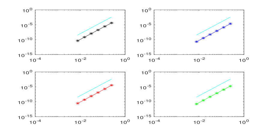
Figure 5.1: Global errors of the numerical solutions by RKN-IIIB method(black line), RKN-Diagsymp method (blue line), RKN-A method (red line) and RKN-B method (green line) for the perturbed pendululm equation (5.4). The reference line has slope 4 in every subplots.

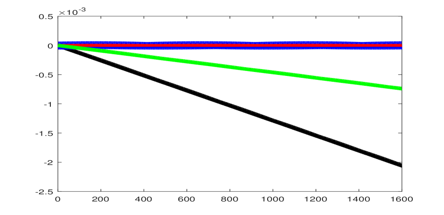
Figure 5.2: Energy errors of the numerical solutions by RKN-IIIB method(black line), RKN-Diagsymp method (blue line), RKN-A method (red line) and RKN-B method (green line) for the perturbed pendululm equation (5.4): step size $h=0.16,$ integration interval $[0,1600].$

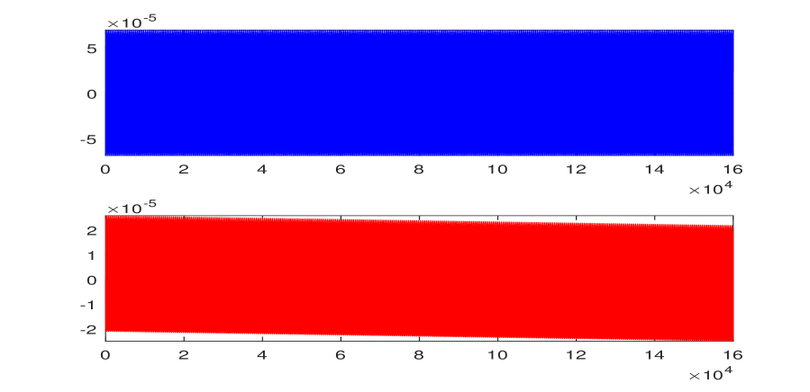
Figure 5.3: Energy errors of the numerical solutions by RKN-Diagsymp method (blue line), and RKN-A method (red line) for the perturbed pendululm equation (5.4): step size $h=0.16,$ integration interval $[0,1.6\times 10^{5}].$

Global errors of the numerical solutions by the above four methods with six small step sizes are shown in Fig. 5.1 with log-log scales, which verifies the order of all the methods. From Fig. 5.2, it is seen that RKN-IIIB method and RKN-B method produce obvious energy drifts, though these methods are symmetric. This shows that not all symmetric RKN methods nearly preserve the energy over long times even if the system is reversible — this observation has been shown for symmetric Runge-Kutta methods in [10]. It is observed that the energy error keeps bounded for the RKN-Diagsymp method. Besides, it seems that the non-symplectic RKN-A method gives a “better” behavior. However, when we integrate the system on a much longer time interval $[0,1.6\times 10^{5}]$, it gives a worse result (energy drift) compared with the RKN-Diagsymp method (see Fig. 5.3). From these numerical tests we may conclude that symplectic-structure preservation is more essential than the reversibility preservation of the reversible Hamiltonian systems in long-term numerical simulation. Nevertheless, for general reversible non-Hamiltonian systems, symmetric methods are also preferable.

6 Concluding remarks

We develop symmetric integrators by means of continuous-stage Runge-Kutta-Nyström (csRKN) methods in this paper. The crucial technique based on Legendre polynomial expansion combining with the symmetric conditions and order conditions is fully utilized. As illustrative examples, new families of symmetric integrators (most of them are also symplectic) are derived in use of Gaussian-type and Lobatto-type quadrature formulas. It is worth observing that other quadrature formulas can also be considered for devising symmetric integrators and more free parameters can be led into the formalism of the Butcher coefficients.

References

• [1] L. Brugnano, F. Iavernaro, D. Trigiante, Hamiltonian boundary value methods: energy preserving discrete line integral methods, J. Numer. Anal., Indust. Appl. Math., 5 (1–2) (2010), 17–37.
• [2] L. Brugnano, F. Iavernaro, D. Trigiante, Analysis of Hamiltonian Boundary Value Methods (HBVMs): A class of energy-preserving Runge CKutta methods for the numerical solution of polynomial Hamiltonian systems, Commun. Nonlinear. Sci. Numer. Simulat., 20 (3) (2015), 650–667.
• [3] L. Brugnano, F. Iavernaro, Line Integral Methods for Conservative Problems, Monographs and Research Notes in Mathematics, CRC Press, Boca Raton, FL, 2016.
• [4] L. Brugnano, F. Iavernaro, D. Trigiante, A simple framework for the derivation and analysis of effective one-step methods for ODEs, Appl. Math. Comput., 218 (2012), 8475–8485.
• [5] L. Brugnano, F. Iavernaro, Line Integral Solution of Differential Problems, Axioms, 7(2) (2018) 36, https://doi.org/10.3390/axioms7020036.
• [6] C. Burnton, R. Scherer, Gauss-Runge-Kutta-Nyström methods, BIT, 38 (1998), 12–21.
• [7] J. R. Cash, A variable step Runge-Kutta-Nyström integrator for reversible systems of second order initial value problems, SIAM J. Sci. Comput., 26 (2005), 963–978.
• [8] E. Celledoni, R. I. McLachlan, D. McLaren, B. Owren, G. R. W. Quispel, W. M. Wright., Energy preserving Runge-Kutta methods, M2AN 43 (2009), 645–649.
• [9] R. P. K. Chan, On symmetric Runge–Kutta methods of high order, Computing, 45 (1990), 301–309.
• [10] E. Faou, E. Hairer, T. L. Pham, Energy Conservation with Non-Symplectic Methods: Examples and Counter-Examples, Bit Numerical Mathematics, 44 (2004), 699–709.
• [11] K. Feng, On difference schemes and symplectic geometry, Proceedings of the 5-th Inter., Symposium of Differential Geometry and Differential Equations, Beijing, 1984, 42–58.
• [12] K. Feng, K. Feng’s Collection of Works, Vol. 2, Beijing: National Defence Industry Press, 1995.
• [13] K. Feng, M. Qin, Symplectic Geometric Algorithms for Hamiltonian Systems, Spriger and Zhejiang Science and Technology Publishing House, Heidelberg, Hangzhou, First edition, 2010.
• [14] E. Hairer, S. P. Nørsett, G. Wanner, Solving Ordiary Differential Equations I: Nonstiff Problems, Springer Series in Computational Mathematics, 8, Springer-Verlag, Berlin, 1993.
• [15] E. Hairer, C. Lubich, G. Wanner, Geometric Numerical Integration: Structure-Preserving Algorithms For Ordinary Differential Equations, Second edition. Springer Series in Computational Mathematics, 31, Springer-Verlag, Berlin, 2006.
• [16] E. Hairer, Energy-preserving variant of collocation methods, JNAIAM J. Numer. Anal. Indust. Appl. Math., 5 (2010), 73–84.
• [17] J. Hong, A survey of multi-symplectic Runge-Kutta type methods for Hamiltonian partial differential equations, Frontiers and prospects of contemporary applied mathematics, 2005, 71–113.
• [18] Y. Li, X. Wu, Functionally fitted energy-preserving methods for solving oscillatory nonlinear Hamiltonian systems, SIAM J. Numer. Anal., 54 (4)(2016), 2036–2059.
• [19] R. I. Mclachlan, G. R. W. Quispel, G. S. Turner, Numerical integrators that preserve symmetries and reversing symmetries, SIAM J. Numer. Anal., 35 (1998), 586–599.
• [20] Y. Miyatake, An energy-preserving exponentially-fitted continuous stage Runge-Kutta methods for Hamiltonian systems, BIT Numer. Math., 54(2014), 777–799.
• [21] Y. Miyatake, J. C. Butcher, A characterization of energy-preserving methods and the construction of parallel integrators for Hamiltonian systems, SIAM J. Numer. Anal., 54(3)(2016), 1993–2013.
• [22] D. Okunbor, RD. Skeel, Explicit canonical methods for Hamiltonian systems, Math. Comput., 59 (1992), 439–455.
• [23] G. R. W. Quispel, D. I. McLaren, A new class of energy-preserving numerical integration methods, J. Phys. A: Math. Theor., 41 (2008) 045206.
• [24] J. M. Sanz-Serna, M. P. Calvo, Numerical Hamiltonian problems, Chapman & Hall, 1994.
• [25] D. Stoffer, Variable steps for reversible integration methods, Computing, 55 (1) (1995), 1–22.
• [26] W. Tang, Y. Sun, A new approach to construct Runge-Kutta type methods and geometric numerical integrators, AIP. Conf. Proc., 1479 (2012), 1291-1294.
• [27] W. Tang, Y. Sun, Time finite element methods: A unified framework for numerical discretizations of ODEs, Appl. Math. Comput. 219 (2012), 2158–2179.
• [28] W. Tang, Y. Sun, Construction of Runge-Kutta type methods for solving ordinary differential equations, Appl. Math. Comput., 234 (2014), 179–191.
• [29] W. Tang, G. Lang, X. Luo, Construction of symplectic (partitioned) Runge-Kutta methods with continuous stage, Appl. Math. Comput. 286 (2016), 279–287.
• [30] W. Tang, Y. Sun, W. Cai, Discontinuous Galerkin methods for Hamiltonian ODEs and PDEs, J. Comput. Phys., 330 (2017), 340–364.
• [31] W. Tang, J. Zhang, Symplecticity-preserving continuous-stage Runge-Kutta-Nyström methods, Appl. Math. Comput., 323 (2018), 204–219.
• [32] W. Tang, Y. Sun, J. Zhang, High order symplectic integrators based on continuous-stage Runge-Kutta-Nyström methods, arXiv:1510.04395 [math.NA], 2018.
• [33] W. Tang, A note on continuous-stage Runge-Kutta methods, Appl. Math. Comput., 339 (2018), 231–241.
• [34] W. Tang, Continuous-stage Runge-Kutta methods based on weighted orthogonal polynomials, arXiv:1805.09955 [math.NA], 2018.
• [35] W. Tang, An extended framework of continuous-stage Runge-Kutta methods, arXiv:1806.05074 [math.NA], 2018.