Controllable spin-Hall and related effects of light in an atomic medium via coupling fields

Abstract

We show the existence of spin-Hall effect of light (SHEL) in an atomic medium which is made anisotropic via electromagnetically induced transparency. The medium is made birefringent by applying an additional linearly polarized coupling light beam. The refractive index and the orientation of the optics axis are controlled by the coupling beam. We show that after transmitting the atomic medium, a linearly polarized probe light beam splits into its two spin components by opposite transverse shifts. With proper choice of parameters and atomic density of about $2.5\times 10^{17}\,\mathrm{m}^{-3}$, the shifts are about the order of wavelength and can be larger than the wavelength by increasing the atomic density. We propose a novel measurement scheme based on a balanced homodyne detection (BHD). By properly choosing the polarization, phase, and transverse mode of the local oscillator of the BHD, one can independently measure (i) the SHEL shifts of the two spin components; (ii) the spatial and angular shifts; (iii) the transverse and longitudinal shifts. The measurement can reach the quantum limit of precision by detecting signals at the modulation frequency of the electro-optic modulator used to modulate the input probe beam. The precision is estimated to be at the nanometer level limited by the quantum noise.

I Introduction

Spin-orbit interaction of light Bliokh et al. (2015a) originates from the fundamental spin properties of Maxwell’s equations, and thus is inherent in all basic optical processes. It yields many fascinating spin-dependent phenomena, in which the spin of light controls the propagation direction Bliokh et al. (2008a); Bliokh (2009); Bliokh et al. (2015b); Gorodetski et al. (2012); Petersen et al. (2014); Junge et al. (2013); Mitsch et al. (2014), the phase and intensity distribution Zhao et al. (2007); Marrucci et al. (2006, 2011); Bliokh et al. (2011); Sukhov et al. (2015), etc. Spin-Hall effect of light (SHEL) Hosten and Kwiat (2008); Onoda et al. (2004); Ling et al. (2017); Haefner et al. (2009); Aiello et al. (2009); Korger et al. (2014), as a typical instance of the spin-orbit interaction of light, has been extensively investigated both theoretically and experimentally in a variety of systems, due to its potential applications in precision metrology Zhou et al. (2012a, b), ultra-fast image processing Zhu et al. (2018), etc. The SHEL manifests as the spin accumulation at the opposite sides of a light beam, or equivalently, the spin-dependent shifts of its centroid. Such shifts occur, for example, when a light beam is reflected or refracted at a planar dielectric interface. Specifically, after reflection or refraction, light beams with right- and left-circular polarizations experience opposite shifts perpendicular to the incident plane, while a linearly polarized light beam splits into its two spin components. The former is the so-called Imbert-Fedorov (IF) shift Bliokh (2013) and the latter is conventionally referred to as SHEL. Similar shifts also appear when a light beam propagates spirally in a smooth gradient-index medium Bliokh et al. (2008a); Bliokh (2009). It has been proven that the total angular momentum, the spin angular momentum plus the orbit angular momentum, is conserved in the SHEL Bliokh and Bliokh (2006). The underlying physics of aforementioned SHEL is the spin-redirection Rytov-Vladimirskii-Berry (PVB) phase Bliokh et al. (2008b) related to the change of the wave vector direction. Besides, another kind of geometric phase, i.e., the Pancharatnam-Berry (PB) phase Bliokh et al. (2008b) associated with the manipulation of the polarization state, also leads to SHEL, where the light beam undergoes spin-dependent momentum shifts (deflection of the propagation direction) Bomzon et al. (2002); Shitrit et al. (2011).

The SHEL at an interface essentially arises from the interplay between the spin-redirection PVB phase and the sharply inhomogeneous refractive index. Actually, the anisotropic refractive index of, e.g. a uniaxial crystal, also induces the SHEL Bliokh et al. (2016). This can be understood from the viewpoint of symmetry because both of them have cylindrically symmetric refractive indexes around the normal of the interface and the optics axis of the uniaxial crystal, respectively. However, in contrast to the interface whose symmetry is geometric, the symmetry of the uniaxial crystal is associated with the intrinsic anisotropy. Therefore, the incident angle is defined with respect to the optics axis. Note that this kind of anisotropy induced SHEL, which is also associated with the spin-redirection PVB phase, is different from the SHEL in a structured anisotropic medium, such as a space-variant subwavelength grating Bomzon et al. (2002), which originates from the space-variant PB phase. Although the SHEL at an interface has been extensively studied, this anisotropy induced SHEL has received little attention.

In this article, we examine how an atomic medium can produce SHEL. This requires making the atomic medium anisotropic, which can be done by applying coupling laser fields and by using the electromagnetically induced transparency (EIT) Fleischhauer et al. (2005); Patnaik and Agarwal (2000). Specifically, the atomic medium exhibits a linear birefringence when a linearly polarized coherent coupling beam is applied. When another linearly polarized probe beam passes through the atomic medium it experiences the SHEL shifts, which can be significantly enhanced by strong absorptive anisotropy. This is in close analogy to the giant transverse shifts near the Brewster angle at an interface Götte et al. (2014); Luo et al. (2011); Xu et al. (2016). We present detailed results not only for SHEL but other kind of shifts like Goos-Hänchen (GH) shifts and the angular shifts Bliokh (2013). Since the shifts are at the subwavelength scale, the experimental detection requires a high measurement precision. In previous investigations, the weak measurement Hosten and Kwiat (2008); Aharonov et al. (1988); Duck et al. (1989); Ritchie et al. (1991); Dressel et al. (2014); Dennis and Götte (2012); Zhou et al. (2012c); Töppel et al. (2013); Goswami et al. (2014) is most widely used, which enlarges the shifts by a factor of several hundreds. Here, we provide a more efficient method to study the SHEL and related shifts based on a balanced homodyne detection (BHD) Hsu et al. (2004); Delaubert et al. (2006); Sun et al. (2014) with a properly chosen local oscillator (LO). We analyze the precision of this method and show that the minimum measurable shift is at the nanometer level under typical experimental conditions and is only limited by the quantum noise.

Our scheme shows three main advantages. First, differently from a natural crystal, e.g. calcite, the optical properties of the atomic medium can be flexibly controlled by the coupling beam. Especially, the orientation of the optics axis can be adjusted without moving the medium. In fact, in order to observe the SHEL solely induced by the anisotropy, the probe beam has to pass through the medium perpendicularly to the surface to avoid the influences of the interface induced SHEL, the GH shift, and the IF shift, and moreover, the optics axis has to be tilted. When the incident angle is varying, it is challenging to realize this in a natural crystal of which the optics axis is fixed, as the situation in Ref. Bliokh et al. (2016). Instead, this is straightforward to be implemented in our scheme. Second, the two spin components undergo a longitudinal shift and opposite transverse SHEL shifts, and all the shifts can be spatial and angular. That is to say, the shifts have three degrees of freedom: (i) the opposite shifts of the two spin components; (ii) the spatial and angular shifts; (iii) the longitudinal and transverse shifts. The traditional quadrant-detector-based measurement combined with the weak-value enhancement only detects the centroid shifts at the position of the detector, which is actually an overall effect of the shifts occurring in these three degrees of freedom. It is difficult for this scheme to fully decompose the overall shift in specific degrees of freedom. Especially, to decompose the spatial and angular shifts, one has to move the detector to perform the measurement at least in two positions. Since the shifts are very small, this probably decreases the precision. However, in our scheme, the shifts in the three degrees of freedom can be independently measured by appropriately choosing the polarization, phase, and transverse mode of the LO. Third, it has been proven that the quadrant detection is about 80% efficiency compared to the BHD to measure the tiny shifts Delaubert et al. (2006); Sun et al. (2014). In our scheme, the BHD-based measurement can reach the quantum limit by suppressing the classical noises using frequency modulation technique.

II Anisotropic EIT medium

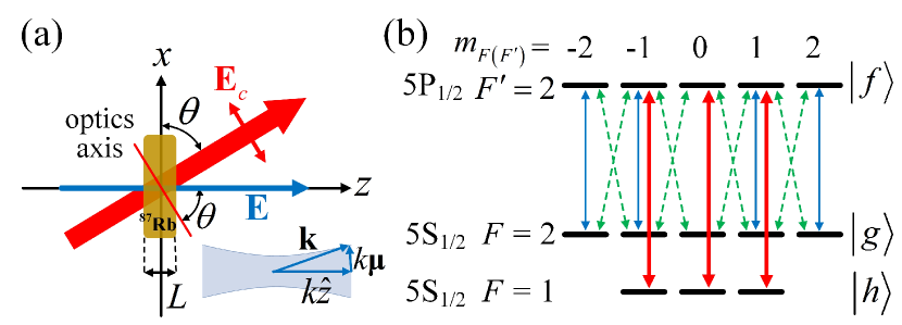
Figure 1: (a) Schematic diagram of the system (see the text for the description). The lower right inset shows the distribution of the wave vector $\mathbf{k}=k(\bm{\mu}+\sqrt{1-|\bm{\mu}|^{2}}\hat{\bm{z}})$ narrowly around the central wave vector $k\hat{\bm{z}}$. (b) Relevant energy levels in the ⁸⁷Rb D1 line. The thin solid blue and dashed green lines represent the $\pi$ and $\sigma^{\pm}$ transitions for the probe beam, respectively. The thick solid red lines represent the $\pi$ transitions for the linearly polarized coupling beam.

We consider an atom-light interaction scheme, as shown in Fig. 1 (a), where the atomic medium with a length of $L$ is composed of ⁸⁷Rb atoms whose D1 line consists of an excited state $\ket{f}=\ket{5\mathrm{P}_{1/2},F^{\prime}=2}$, and two ground states $\ket{g}=\ket{5\mathrm{S}_{1/2},F=2}$ and $\ket{h}=\ket{5\mathrm{S}_{1/2},F=1}$, as illustrated in Fig. 1 (b). A monochromatic probe Gaussian beam propagating along the $z$-axis passes through the medium and acts on the transition $\ket{f}\leftrightarrow\ket{g}$. Its electric field $\mathbf{E}_{p}\propto\hat{\bm{\epsilon}}u(x,y)e^{-i\nu t+ikz}$, with $\hat{\bm{\epsilon}}$ the polarization vector, $\nu$ the frequency, $k=\nu/c$ the wave number, $c$ the speed of light in vacuum, $u(x,y)=w_{0}^{-1}e^{-(x^{2}+y^{2})/w_{0}^{2}}$ the amplitude distribution in the position space, and $w_{0}$ the beam waist. Such a spatially confined light can be taken as a superposition of plane waves: $\mathbf{E}_{p}\propto\int\tilde{\mathbf{E}}_{p}\mathrm{d}k_{x}\mathrm{d}k_{y}=\hat{\bm{\epsilon}}\int\tilde{u}(k_{x},k_{y})e^{-i\nu t+i\mathbf{k}\cdot\mathbf{r}}\mathrm{d}k_{x}\mathrm{d}k_{y}$ with the position vector $\mathbf{r}=x\hat{\bm{x}}+y\hat{\bm{y}}+z\hat{\bm{z}}$ and the wave vector $\mathbf{k}=k\hat{\mathbf{k}}=k(\bm{\mu}+\sqrt{1-|\bm{\mu}|^{2}}\hat{\bm{z}})$ narrowly distributed around the central wave vector $k\hat{\bm{z}}$, where $\bm{\mu}=(k_{x}\hat{\bm{x}}+k_{y}\hat{\bm{y}})/k=\mu_{x}\hat{\bm{x}}+\mu_{y}\hat{\bm{y}}$, and $|\bm{\mu}|\ll 1$, as shown in the inset of Fig. 1 (a). Here $\hat{\bm{x}}$, $\hat{\bm{y}}$, and $\hat{\bm{z}}$ are the unit vectors along the $x$-, $y$-, and $z$-axis, respectively. $\tilde{u}(k_{x},k_{y})=w_{0}/2e^{-w_{0}^{2}(k_{x}^{2}+k_{y}^{2})/4}$ is the Fourier transform of $u(x,y)$, representing the amplitude distribution in the momentum space.

An additional linearly polarized strong coupling beam, resonant with the transition $\ket{f}\leftrightarrow\ket{h}$, is applied to prepare the atomic medium to be anisotropic. The coupling beam propagates along the direction at an angle $\theta$ to the $x$-axis, as illustrated in Fig. 1 (a). The beam width is large enough that in the medium the region where the atoms interact with the probe beam is fully covered by the coupling beam. We treat this coupling beam as a plane wave: $\mathbf{E}_{c}=\mathcal{E}_{c}\hat{\bm{\epsilon}}_{c}e^{-i\nu_{c}t+i\rm{k}_{c}\cdot\rm{r}}$ with $\mathcal{E}_{c}$ the amplitude, $\nu_{c}$ the frequency, $\hat{\bm{\epsilon}}_{c}=\hat{\bm{x}}\sin{\theta}-\hat{\bm{z}}\cos{\theta}$ the polarization vector, and $\bm{k}_{c}=k_{c}(\hat{\bm{x}}\cos{\theta}+\hat{\bm{z}}\sin{\theta})$ the wave vector.

Firstly, we consider the action of the atomic medium on the central plane-wave component of the probe beam and then show the SHEL in the next section. The quantization axis is taken to be parallel to $\hat{\bm{\epsilon}}_{c}$, and thus the coupling beam is $\pi$-polarized and couples the $\pi$ transitions between $\ket{f}$ and $\ket{h}$ as indicated by the red lines in Fig. 1 (b). For the special case of $\theta=\pi/2$, when the plane wave is linearly polarized along the $x$-axis (denoted by $\ket{x}$), i.e., parallel to the quantization axis, it couples the $\pi$ transitions between $\ket{f}$ and $\ket{g}$ as indicated by the blue lines. In this case, the system can be considered as a superposition of two three-level $\Lambda$-type EIT ($\ket{g,m_{F}=\pm 1}\leftrightarrow\ket{f,m_{F^{\prime}}=\pm 1}\leftrightarrow\ket{h,m_{F}=\pm 1}$) and two two-level ($\ket{g,m_{F}=\pm 2}\leftrightarrow\ket{f,m_{F^{\prime}}=\pm 2}$) subsystems. The plane wave experiences a refractive index of $n_{x}=\sqrt{1+\chi_{\pi}}$ with the susceptibility

$$\chi_{\pi}=\sum_{i=\pm 1}\kappa_{f_{i}g_{i}}\frac{\xi_{hg}\rho_{g_{i}g_{i}}}{\xi_{fg}\xi_{hg}-|\Omega_{f_{i}h_{i}}|^{2}}+\sum_{i=\pm 2}\kappa_{f_{i}g_{i}}\frac{\rho_{g_{i}g_{i}}}{\xi_{fg}},$$ (1)

where the first (second) term denotes the susceptibilities of the three- (two-) level subsystems, and $\xi_{fg}=\delta-i\Gamma_{fg}$, $\xi_{hg}=\delta-i\Gamma_{hg}$, $\kappa_{f_{i}g_{i}}=N_{a}|\mathbf{d}_{f_{i}g_{i}}|^{2}/(\varepsilon_{0}\hbar)$, $\Omega_{f_{i}h_{i}}=\mathcal{E}_{c}\mathbf{d}_{f_{i}h_{i}}\cdot\hat{\bm{\epsilon}}_{c}/\hbar$ is the Rabi frequency of the coupling field, and $\rho_{g_{i}g_{i}}$ is the population of $\ket{g,m_{F}=i}$. Here $\delta=\omega_{fg}-\nu$ is the detuning of the probe beam with $\omega_{fg}$ the resonant frequency of transition $\ket{f}\leftrightarrow\ket{g}$, $\Gamma_{fg}=\gamma_{fg}$ and $\Gamma_{hg}\approx 0$ are the decay rates of the off-diagonal density matrix elements $\rho_{fg}$ and $\rho_{hg}$, respectively, $2\gamma_{fg}$ is the spontaneous decay rate from $\ket{f}$ to $\ket{g}$, $\mathbf{d}_{f_{i}g_{i}}$ and $\mathbf{d}_{f_{i}h_{i}}$ are the dipole matrix elements of the transitions $\ket{f,m_{F^{\prime}}=i}\leftrightarrow\ket{g,m_{F}=i}$ and $\ket{f,m_{F^{\prime}}=i}\leftrightarrow\ket{h,m_{F}=i}$, respectively, $N_{a}$ is the atomic number density, $\varepsilon_{0}$ is the vacuum permittivity, and $\hbar$ is reduced Planck constant.

When the plane wave is linearly polarized along the $y$-axis (denoted by $\ket{y}$), i.e., perpendicular to the quantization axis, it is a superposition of $\sigma^{+}$- and $\sigma^{-}$-polarized lights and thus couples the $\sigma^{+}$ and $\sigma^{-}$ transitions between $\ket{f}$ and $\ket{g}$ as indicated by the green lines in Fig. 1 (b). In this case, the system can be considered as a superposition of six three-level $\Lambda$-type EIT [$\ket{g,m_{F}=-2,-1,0}$ ($\ket{g,m_{F}=0,1,2}$)$\leftrightarrow\ket{f,m_{F^{\prime}}=-1,0,1}\leftrightarrow\ket{h,m_{F}=-1,0,1}$] and two two-level ($\ket{g,m_{F}=\pm 1}\leftrightarrow\ket{f,m_{F^{\prime}}=\pm 2}$) subsystems. The plane wave experiences a refractive index of $n_{y}=\sqrt{1+\chi_{\sigma}}$ with the susceptibility

$$\chi_{\sigma}=\frac{1}{2}\Bigg{[}\sum_{i=-2}^{0}\kappa_{f_{i+1}g_{i}}\frac{\xi_{hg}\rho_{g_{i}g_{i}}}{\xi_{fg}\xi_{hg}-|\Omega_{f_{i+1}h_{i+1}}|^{2}}+\kappa_{f_{2}g_{1}}\frac{\rho_{g_{1}g_{1}}}{\xi_{fg}}$$

$$+\sum_{i=0}^{2}\kappa_{f_{i-1}g_{i}}\frac{\xi_{hg}\rho_{g_{i}g_{i}}}{\xi_{fg}\xi_{hg}-|\Omega_{f_{i-1}h_{i-1}}|^{2}}+\kappa_{f_{-2}g_{-1}}\frac{\rho_{g_{-1}g_{-1}}}{\xi_{fg}}\Bigg{]},$$ (2)

where the first and third (second and forth) terms denote the susceptibilities of the three- (two-) level subsystems.

In the general case when $\theta$ is arbitrary, for the plane wave with polarization $\ket{x}$, its projections parallel and perpendicular to the quantization axis, which depend on $\theta$, couple the $\pi$ and $\sigma$ transitions between $\ket{f}$ and $\ket{g}$, respectively. However, for the plane wave with polarization $\ket{y}$, it is always perpendicular to the quantization axis regardless of $\theta$ and thus it still couples the $\sigma$ transitions. As a result, the refractive index for the $\ket{x}$ polarization is a function of $\theta$, while that for the $\ket{y}$ polarization is independent of $\theta$ (see Appendix A):

$$n_{x}(\theta)=\sqrt{\frac{\varepsilon_{\sigma}\varepsilon_{\pi}}{\varepsilon_{\sigma}\sin^{2}{\theta}+\varepsilon_{\pi}\cos^{2}{\theta}}},\quad n_{y}=\sqrt{\varepsilon_{\sigma}},$$ (3)

where $\varepsilon_{\pi(\sigma)}=1+\chi_{\pi(\sigma)}$ is the relative permittivity. After passing through the atomic medium, the central plane waves with polarization $\ket{x}$ and $\ket{y}$ evolve as:

$$\ket{x}\rightarrow e^{i\phi_{x}(\theta)}\ket{x},\quad\ket{y}\rightarrow e^{i\phi_{y}}\ket{y},$$ (4)

where $\phi_{x}(\theta)=n_{x}(\theta)kL$ and $\phi_{y}=n_{y}kL$, of which the real and imaginary parts represent the phase shifts and the absorptions.

Without the coupling beam ($\Omega_{f_{i}h_{i}}=0$), $n_{x}=n_{y}$ and $n_{x}$ is independent of $\theta$, i.e., the atomic medium becomes isotropic. The presence of the coupling beam together with the difference of the transition strengths, which are determined by the dipole matrix elements, leads to $n_{x}(\theta)\neq n_{y}$ and the $\theta$-dependence, denoting that the refractive index depends on the polarization and the propagation direction of the probe beam. In other words, the atomic medium is linearly birefringent with an optics axis along the direction of the polarization of the coupling beam. It thus can be regarded as a controllable wave plate whose optics axis and refractive index are controlled by the coupling beam.

For the following results to be discussed, we have adopted experimentally feasible parameters: wavelength $\lambda=2\pi/k=794.98\,\mathrm{nm}$, reduced dipole matrix element $d=2.54\times 10^{-29}\,\mathrm{C\cdot m}$, spontaneous decay rates $2\gamma_{fg}=2\gamma=2\pi\times 5.75\,\mathrm{MHz}$, atomic number density $N_{a}=1.0\times 10^{17}\,\mathrm{m}^{-3}$, atomic medium length $L=1\,\mathrm{mm}$, and reduced Rabi frequency of the coupling field $\Omega=\mathcal{E}_{c}d/\hbar=5\gamma$. The Rabi frequencies $\Omega_{f_{i}h_{i}}$ and the factors $\kappa_{f_{i}g_{i}}$ in Eqs. (1) and (2) can then be calculated using the Clebsch-Gordan coefficients (see Appendix B). The population $\rho_{g_{i}g_{i}}$ is obtained by numerically solving the density-matrix equations using the AtomicDensityMatrix package provided in Ref. ADM .

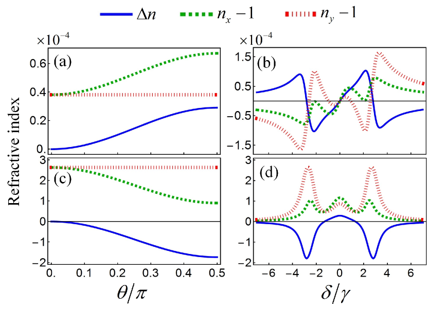
Figure 2: (a), (b) Real and (c), (d) imaginary parts of $\Delta n$, $n_{x}-1$, and $n_{y}-1$ versus $\theta$ and $\delta$ with (a), (c) $\delta=2.7\gamma$ and (b), (d) $\theta=\pi/2$, respectively. See text for the details of the other parameters.

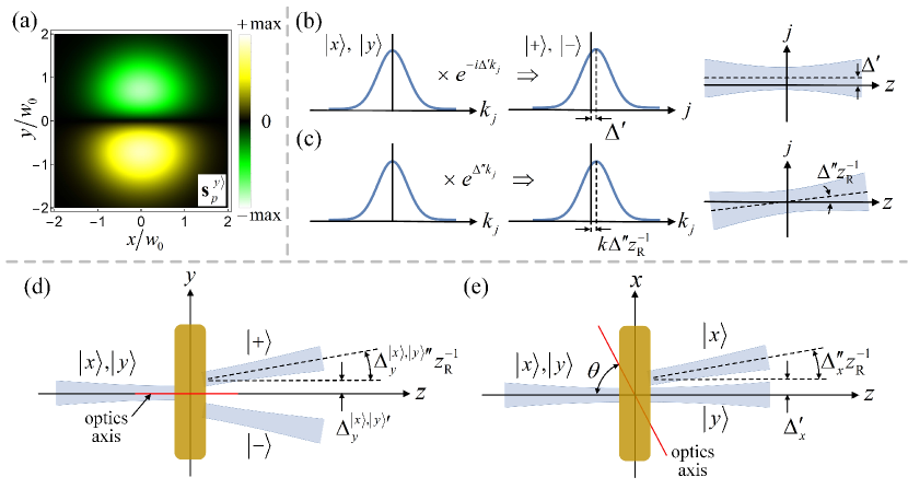
Figure 3: Atomic SHEL and GH shifts. (a) Spin density distribution of $\mathbf{E}_{p}^{\ket{y}}$ showing the spin accumulation. (b) A phase modulation of $e^{-i\Delta^{\prime}k_{j}}$ ($\Delta^{\prime}\equiv\mathrm{Re}\Delta,j=x,y$) in the momentum space leads to a spatial shift of $\Delta^{\prime}$ along the $j$-axis in the position space. (c) A amplitude modulation of $e^{\Delta^{\prime\prime}k_{j}}$ ($\Delta^{\prime\prime}\equiv\mathrm{Im}\Delta$) leads to a shift of $k\Delta^{\prime\prime}/z_{\mathrm{R}}$ along the $k_{j}$-axis in the momentum space which results in a angular shift of $\Delta^{\prime\prime}/z_{\mathrm{R}}$ in the $jz$-plane of the position space. (d) The transmitted probe beam splits into its two spin components $\ket{+}$ and $\ket{-}$ by opposite spatial shifts of $\pm\Delta_{y}^{\ket{x},\ket{y}^{\prime}}$ and angular shifts of $\pm\Delta_{y}^{\ket{x},\ket{y}^{\prime\prime}}/z_{\mathrm{R}}$ along the $y$-axis. (e) The transmitted probe beam with $\ket{x}$ polarization experiences an overall spatial shift of $\Delta_{x}^{\prime}$ and a angular shift of $\Delta_{x}^{\prime\prime}/z_{\mathrm{R}}$ along the $x$-axis, while the one with $\ket{y}$ polarization does not experience such shift. All the shifts are exaggerated.

The anisotropy of the atomic medium is characterized by the difference of $n_{x}(\theta)$ and $n_{y}$: $\Delta n(\theta)=n_{x}(\theta)-n_{y}$, of which the real and imaginary parts are responsible for the dispersive and absorptive anisotropies, respectively. When $\theta=0$, both the $\ket{x}$- and $\ket{y}$-polarization plane waves couple the $\sigma$ transitions between $\ket{f}$ and $\ket{g}$, and they experience the same refractive index, i.e., $n_{x}(0)=n_{y}=\sqrt{\varepsilon_{\sigma}}$ [see Eq. (3)] and $\Delta n(0)=0$. When $\theta=\pi/2$, they couple the $\pi$ and $\sigma$ transitions, respectively, and one has $n_{x}(\pi/2)=\sqrt{\varepsilon_{\pi}}$, $n_{y}=\sqrt{\varepsilon_{\sigma}}$, and a maximum $\Delta n(\pi/2)$. $\Delta n(\theta)$ grows with $\theta$ ranging from 0 to $\pi/2$, as shown in Fig. 2 (a) and (c). From Fig. 2 (b) and (d), it is seen that the atomic medium exhibits weak anisotropy around $\delta=0$ and relative strong anisotropy near $\delta=\pm 2.8\gamma$. The former (the latter) is due to the difference between the two- (three-) level-subsystem susceptibilities of $\chi_{\pi}$ and $\chi_{\sigma}$ [see Eqs. (1) and (2)]. The shifts of $\pm 2.8\gamma$ from the resonant frequency are a joint result of the Autler-Townes splitting Cohen-Tannoudji et al. (1998) of $\pm\Omega_{f_{\pm 1}h_{\pm 1}}=\pm 0.5\Omega=\pm 2.5\gamma$ and $\pm\Omega_{f_{0}h_{0}}=\pm\Omega/\sqrt{3}\approx\pm 2.9\gamma$ (see Appendix A).

III Atomic SHEL and GH shifts

We now consider the action of the atomic medium on an arbitrary plane-wave component of the probe beam and show the SHEL. Equation (4) needs slight modifications for $\bm{\mu}\neq 0$. The plane-wave component with $\mu_{x}\neq 0$ and $\mu_{y}=0$ propagates at a different angle $\theta+\mu_{x}$ to the optics axis, which slightly modifies the Eq. (4): $\ket{x}\rightarrow e^{i\phi_{x}(\theta)}e^{-i\Delta_{x}k_{x}}\ket{x}$ and $\ket{y}\rightarrow e^{i\phi_{y}}\ket{y}$ with $\Delta_{x}=-k^{-1}\partial\phi_{x}(\theta)/\partial\theta$. If further $\mu_{y}\neq 0$, the plane-wave component propagates in a slightly different plane, which can be obtained by rotating the $xz$-plane an angle $\mu_{y}/\sin{\theta}$ around the optics axis. Such a rotation induces spin-redirection PVB geometric phases of $\phi_{\mathrm{G}}=\mp\mu_{y}\cot{\theta}$ for the right- and left-circularly polarized plane-wave components, respectively, which is associated with the spin-orbit interaction Bliokh et al. (2015a); Bliokh (2013). As a result, after the action of the atomic medium, $\ket{y}$ ($\ket{x}$) polarization is mixed into the plane-wave component with $\ket{x}$ ($\ket{y}$) polarization (see Appendix C): $\ket{x}\rightarrow e^{i\phi_{x}(\theta)}e^{-i\Delta_{x}k_{x}}(\ket{x}+\Delta_{y}^{\ket{x}}k_{y}\ket{y})$ and $\ket{y}\rightarrow e^{i\phi_{y}}(\ket{y}-\Delta_{y}^{\ket{y}}k_{y}\ket{x})$ with $\Delta_{y}^{\ket{x}}=k^{-1}(1-e^{-i\phi(\theta)})\cot{\theta}$, $\Delta_{y}^{\ket{y}}=k^{-1}(1-e^{i\phi(\theta)})\cot{\theta}$, and $\phi(\theta)=\phi_{x}(\theta)-\phi_{y}$. Similar results for the interface can be found in Ref. Hosten and Kwiat (2008).

III.1 Spin Accumulation

In the momentum space, the probe beams with polarizations $\ket{x}$ and $\ket{y}$ evolve to

$$\tilde{\mathbf{E}}_{p}^{\ket{x}} \propto e^{-i\Delta_{x}k_{x}}\tilde{u}\big{(}k_{x},k_{y}\big{)}\big{(}\ket{x}+\Delta_{y}^{\ket{x}}k_{y}\ket{y}\big{)},$$

$$\tilde{\mathbf{E}}_{p}^{\ket{y}} \propto\tilde{u}\big{(}k_{x},k_{y}\big{)}\big{(}\ket{y}-\Delta_{y}^{\ket{y}}k_{y}\ket{x}\big{)},$$ (5)

respectively. The factors $e^{i\phi_{x}(\theta)}$ for $\tilde{\mathbf{E}}_{p}^{\ket{x}}$ and $e^{i\phi_{y}}$ for $\tilde{\mathbf{E}}_{p}^{\ket{y}}$ have been omitted for clarity. Transforming them back to the position space, we obtain (up to first order in $\Delta_{x}$, $\Delta_{y}^{\ket{x}}$ , and $\Delta_{y}^{\ket{y}}$)

$$\mathbf{E}_{p}^{\ket{x}} \propto u\big{(}x-\Delta_{x},y\big{)}\big{(}\ket{x}+2i\Delta_{y}^{\ket{x}}w_{0}^{-2}y\ket{y}\big{)},$$

$$\mathbf{E}_{p}^{\ket{y}} \propto u\big{(}x,y\big{)}\big{(}\ket{y}-2i\Delta_{y}^{\ket{y}}w_{0}^{-2}y\ket{x}\big{)}.$$ (6)

Due to the $y$-dependent terms, the transmitted probe beams are no longer linearly polarized. Instead, they exhibit a distribution of elliptical polarization. For example, when $\Delta_{y}^{\ket{y}}$ has a positive real part, the polarization of $\mathbf{E}_{p}^{\ket{y}}$ is left- (right-) handed elliptical polarization at $y>0$ ($y<0$). This effect can be well described by the spin density Bliokh and Nori (2015); Aiello et al. (2015); Neugebauer et al. (2018)

$$\mathbf{s}_{p}^{\ket{x},\ket{y}} =\frac{1}{4\nu}\mathrm{Im}\bigg{[}\varepsilon_{0}(\mathbf{E}_{p}^{\ket{x},\ket{y}})^{*}\times\mathbf{E}_{p}^{\ket{x},\ket{y}}$$

$$+\mu_{0}(\mathbf{H}_{p}^{\ket{x},\ket{y}})^{*}\times\mathbf{H}_{p}^{\ket{x},\ket{y}}\bigg{]},$$ (7)

where $\mathbf{H}_{p}^{\ket{x},\ket{y}}=\sqrt{\varepsilon_{0}/\mu_{0}}\hat{\mathbf{k}}\times\mathbf{E}_{p}^{\ket{x},\ket{y}}$ is the magnetizing field and $\mu_{0}$ is the vacuum permeability. The spin densities of the linearly and circularly polarized fields are zero and maximum, respectively, while that of the elliptically polarized field is intermediate between them. Right- and left-circular (elliptical) polarizations have opposite spin densities. From Eqs. (6) and (7), we see that $\mathbf{s}_{p}^{\ket{x},\ket{y}}$ only has $z$-component:

$$\mathbf{s}_{p}^{\ket{x}}\propto\Delta_{y}^{\ket{x}^{\prime}}yu^{2}(x-\Delta_{x},y)\hat{\mathbf{z}},\,\,\,\mathbf{s}_{p}^{\ket{y}}\propto\Delta_{y}^{\ket{y}^{\prime}}yu^{2}(x,y)\hat{\mathbf{z}},$$ (8)

with $\Delta_{y}^{\ket{x},\ket{y}^{\prime}}\equiv\mathrm{Re}(\Delta_{y}^{\ket{x},\ket{y}})$, which implies a longitudinal spin. Fig. 3 (a) gives the spin density distribution $\mathbf{s}_{p}^{\ket{y}}$ of $\mathbf{E}_{p}^{\ket{y}}$ (the behavior of $\mathbf{s}_{p}^{\ket{x}}$ is almost the same as that of $\mathbf{s}_{p}^{\ket{y}}$). Obviously, the accumulation of the opposite spins occurs at the two sides of the transmitted probe beam along the $y$-axis, i.e., the SHEL is observed.

III.2 SHEL and GH Shifts

The spin accumulation signifies opposite shifts along the $y$-axis of each spin components. Actually, in the spin basis $\ket{\pm}=(\ket{x}+i\ket{y})/\sqrt{2}$, Eq. (5) can be rewritten as

$$\tilde{\mathbf{E}}_{p}^{\ket{x}} \propto e^{-i\Delta_{x}k_{x}-i\Delta_{y}^{\ket{x}}k_{y}}\tilde{u}\big{(}k_{x},k_{y}\big{)}\ket{+}$$

$$+e^{-i\Delta_{x}k_{x}+i\Delta_{y}^{\ket{x}}k_{y}}\tilde{u}\big{(}k_{x},k_{y}\big{)}\ket{-},$$

$$\tilde{\mathbf{E}}_{p}^{\ket{y}} \propto e^{-i\Delta_{y}^{\ket{y}}k_{y}}\tilde{u}\big{(}k_{x},k_{y}\big{)}\ket{+}$$

$$-e^{i\Delta_{y}^{\ket{y}}k_{y}}\tilde{u}\big{(}k_{x},k_{y}\big{)}\ket{-},$$ (9)

provided that $\big{|}\Delta_{y}^{\ket{x},\ket{y}}\big{|}\ll w_{0}$. In general, $\Delta_{x}$, $\Delta_{y}^{\ket{x}}$, and $\Delta_{y}^{\ket{y}}$ are complex. The real part $\Delta^{\prime}\equiv\mathrm{Re}\Delta$ ($\Delta$ denotes $\Delta_{x}$, $\Delta_{y}^{\ket{x}}$, or $\Delta_{y}^{\ket{y}}$) corresponds to a phase modulation of $e^{-i\Delta^{\prime}k_{j}}$ ($j=x,y$) in the momentum space, which leads to a spatial shift of $\Delta^{\prime}$ along the $j$-axis in the position space: $\int e^{-i\Delta^{\prime}k_{j}}\tilde{u}(k_{j})\mathrm{d}k_{j}=u(j-\Delta^{\prime})$, as illustrated in Fig. 3 (b). The imaginary part $\Delta^{\prime\prime}\equiv\mathrm{Im}\Delta$ corresponds to an amplitude modulation of $e^{\Delta^{\prime\prime}k_{j}}$, which results in a shift of $k\Delta^{\prime\prime}/z_{\mathrm{R}}$ along the $k_{j}$-axis in the momentum space: $e^{\Delta^{\prime\prime}k_{j}}\tilde{u}(k_{j})\approx\tilde{u}(k_{j}-k\Delta^{\prime\prime}/z_{\mathrm{R}})$ with $z_{\mathrm{R}}=kw_{0}^{2}/2$ the Rayleigh range, or equivalently, an angular shift of $\Delta^{\prime\prime}/z_{\mathrm{R}}$ in the $jz$-plane of the position space: $\int e^{\Delta^{\prime\prime}k_{j}}\tilde{u}(k_{j})\mathrm{d}k_{j}=u(j)e^{ikj\Delta^{\prime\prime}/z_{\mathrm{R}}}$, as shown in Fig. 3 (c). In the position space, we have

$$\mathbf{E}_{p}^{\ket{x}} \propto u\big{(}x-\Delta_{x},y-\Delta_{y}^{\ket{x}}\big{)}\ket{+}$$

$$+u\big{(}x-\Delta_{x},y+\Delta_{y}^{\ket{x}}\big{)}\ket{-},$$

$$\mathbf{E}_{p}^{\ket{y}} \propto u\big{(}x,y-\Delta_{y}^{\ket{y}}\big{)}\ket{+}-u\big{(}x,y+\Delta_{y}^{\ket{y}}\big{)}\ket{-},$$ (10)

with the complex shifts of $\Delta_{x}$, $\Delta_{y}^{\ket{x}}$, and $\Delta_{y}^{\ket{y}}$. Equation (10) indicates that the transmitted probe beam with $\ket{x}$ ($\ket{y}$) polarization indeed splits by opposite shifts of $\pm\Delta_{y}^{\ket{x}}$ ($\pm\Delta_{y}^{\ket{y}}$) along the $y$-axis into its two spin components $\ket{+}$ and $\ket{-}$, as shown in Fig. 3 (d). These shifts arise from the factors $e^{\pm i\Delta_{y}^{\ket{x}}k_{y}}$($e^{\pm i\Delta_{y}^{\ket{y}}k_{y}}$) which represent a coupling between the spin and the transverse momentum $k_{y}$. This spin-orbit interaction is a result of the geometric phase as mentioned above. $\Delta_{x}$ represents an overall longitudinal shift along the $x$-axis only for $\ket{x}$ polarization, as shown in Fig. 3 (e). It arises from the factor $e^{-i\Delta_{x}k_{x}}$ in Eq. (9) which originates from the angular gradient of $n_{x}(\theta)$. This indicates that this shift is the atomic counterpart of the GH shift of the reflected beam at an interface.

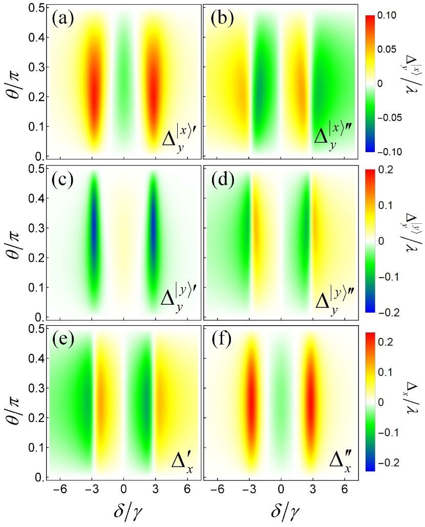
Figure 4: (a)-(d) $\Delta_{y}^{\ket{x},\ket{y}}$ and (e)-(f) $\Delta_{x}$ versus $\delta$ and $\theta$. The other parameters are as in Fig. 2. These are the quantities measured directly by the scheme shown in Fig. 6

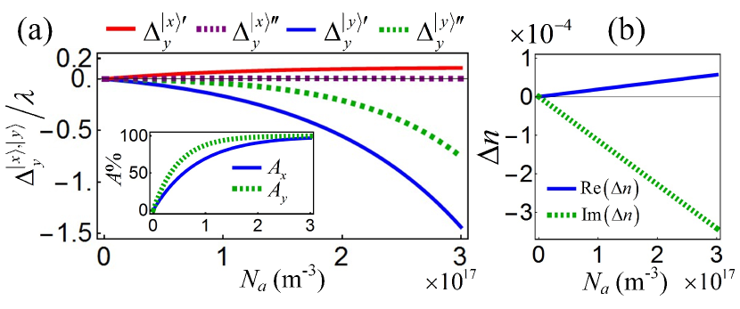
Figure 5: (a) $\Delta_{y}^{\ket{x},\ket{y}}$, (inset) $A_{x,y}$, and (b) $\Delta n$ versus $N_{a}$ with $\delta=2.7\gamma$ and $\theta=0.3\pi$. The other parameters are as in Fig. 2.

Nonzero SHEL ($\Delta_{y}^{\ket{x},\ket{y}}\neq 0$) requires two conditions: (i) the difference between the refractive indexes for the $\ket{x}$- and $\ket{y}$-polarization plane waves, i.e., $\Delta n(\theta)\neq 0$; (ii) nonzero geometric phases for the spin components, i.e., $\phi_{\mathrm{G}}=\mp\mu_{y}\cot{\theta}\neq 0$. For $\theta=0$ and $\pi/2$, one has $\Delta n=0$ and $\phi_{\mathrm{G}}=0$, respectively, and thus $\Delta_{y}^{\ket{x},\ket{y}}=0$, as shown in Fig. 4 (a)-(d). Nonzero $\Delta_{x}$ requires nonzero angular gradient of $n_{x}(\theta)$, i.e., $\partial n_{x}(\theta)/\partial\theta\neq 0$. Similar to the SHEL, for $\theta=0$ and $\pi/2$, one has $\partial n_{x}(\theta)/\partial\theta=0$ [see Fig. 2 (a) and (c)] and thus $\Delta_{x}=0$, as shown in Fig. 4 (e)-(f).

Since these shifts are induced by the anisotropy, large shifts are expected around $\delta=0$ and $\pm 2.8\gamma$, as shown in Fig. 4. We note that the SHEL shifts increase remarkably with the absorptive anisotropy. In order to show this feature, here we give the explicit expressions of the SHEL shifts:

$$\Delta_{y}^{\ket{x}^{\prime}} =k^{-1}(1-e^{\phi^{\prime\prime}}\cos{\phi^{\prime}})\cot{\theta},$$

$$\Delta_{y}^{\ket{x}^{\prime\prime}} =k^{-1}e^{\phi^{\prime\prime}}\sin{\phi^{\prime}}\cot{\theta},$$

$$\Delta_{y}^{\ket{y}^{\prime}} =k^{-1}(1-e^{-\phi^{\prime\prime}}\cos{\phi^{\prime}})\cot{\theta},$$

$$\Delta_{y}^{\ket{y}^{\prime\prime}} =-k^{-1}e^{-\phi^{\prime\prime}}\sin{\phi^{\prime}}\cot{\theta},$$ (11)

with $\phi^{\prime}\equiv\mathrm{Re}\phi$ and $\phi^{\prime\prime}\equiv\mathrm{Im}\phi$, which represent the dispersive and absorptive anisotropies, respectively. The factor $e^{\phi^{\prime\prime}}$ ($e^{-\phi^{\prime\prime}}$) yields a significant enhancement of $\Delta_{y}^{\ket{x}}$ ($\Delta_{y}^{\ket{y}}$ ) for a large positive (negative) value of $\phi^{\prime\prime}$. The parameters used in the calculation yield a large negative value of $\phi^{\prime\prime}=\mathrm{Im}(\Delta n)kL$ near $\delta=\pm 2.8\gamma$ [see Fig. 2 (d)], and thus a large $\Delta_{y}^{\ket{y}}$ [see Fig. 4 (c)-(d)]. A straightforward way to enhance $\phi^{\prime\prime}$ is to increase $N_{a}$, as shown in Fig. 5, but the price to pay is a higher loss of the probe beam [see the inset of Fig. 5 (a) where the absorption is defined as $A_{x,y}=1-e^{-\mathrm{Im}\phi_{x,y}}$ for the $\ket{x}$- and $\ket{y}$-polarization, respectively]. As discussed in the next section, a lower transmitted power reduces the measurement precision. Therefore, there is a trade-off between the large SHEL shifts and the high precision.

IV Measurement scheme of SHEL based on a BHD

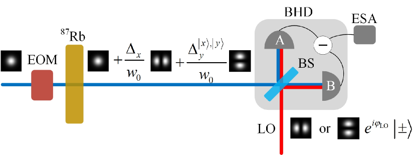
Figure 6: Schematic diagram of the measurement scheme. The shifts of the transmitted probe beam are measured by the BHD with a TEM₁₀ (TEM₀₁) LO. The measurement is performed at RF frequency by using an EOM to modulate the probe beam. EOM: electro-optic modulator; ESA: electronic spectrum analyzer; BS: 50/50 beam splitter.

Obviously, the measurement of the tiny SHEL and GH shifts, at the subwavelength scale (see Fig. 4), requires the sensitivity at the nanometer level. In addition, there are six shifts in all [Fig. 3 (d) and (e)], and thus a full characterization means independent measurement of each one. The traditional quadrant-detector-based measurement combined with the weak-value enhancement fails to meet the second requirement. Therefore, here we present a BHD-based measurement scheme, as schematically illustrated in Fig. 6, which allows to independently measure each shift with a high precision.

Any spatial or angular shift of a fundamental Gaussian beam (TEM₀₀ mode) leads to excitations of higher Hermit-Gaussian modes (TEM_mn modes). Up to first order, the electric field of the transmitted probe beam can be expanded as:

$$\mathbf{E}_{p}^{\ket{x}} \propto\sqrt{\frac{N_{p}}{2}}\left[u_{00}(x,y)+\frac{\Delta_{x}}{w_{0}}u_{10}(x,y)+\frac{\Delta_{y}^{\ket{x}}}{w_{0}}u_{01}(x,y)\right]\ket{+}\sqrt{\frac{N_{p}}{2}}\left[u_{00}(x,y)+\frac{\Delta_{x}}{w_{0}}u_{10}(x,y)-\frac{\Delta_{y}^{\ket{x}}}{w_{0}}u_{01}(x,y)\right]\ket{-},$$

$$\mathbf{E}_{p}^{\ket{y}} \propto\sqrt{\frac{N_{p}}{2}}\left[u_{00}(x,y)+\frac{\Delta_{y}^{\ket{y}}}{w_{0}}u_{01}(x,y)\right]\ket{+}+\sqrt{\frac{N_{p}}{2}}\left[u_{00}(x,y)-\frac{\Delta_{y}^{\ket{y}}}{w_{0}}u_{01}(x,y)\right]\ket{-},$$ (12)

where $u_{10}(x,y)$ and $u_{01}(x,y)$ denote, respectively, the TEM₁₀ and TEM₀₁ Hermit-Gaussian modes, and $N_{p}$ is the mean number of the photons detected in the time interval of one measurement, which is determined by the resolution bandwidth of the measurement device. Equation (12) shows that the excited TEM₁₀ and TEM₀₁ modes carry the information of the shifts along the $x$- and $y$-axis, respectively. This can be extracted by using a TEM₁₀ or TEM₀₁ LO: $\mathbf{E}_{\mathrm{LO}}\propto\sqrt{N_{\mathrm{LO}}}u_{10,01}(x,y)e^{i\varphi_{\mathrm{LO}}}\ket{\pm}$ with $\varphi_{\mathrm{LO}}$ the phase, and $N_{\mathrm{LO}}$ the mean photon number. Since TEM₁₀ and TEM₀₁ modes are orthogonal to each other, a BHD with a TEM₁₀ (TEM₀₁) LO measures the shift along the $x$- ($y$-) axis. In addition, the polarization of the LO determines which spin component of the transmitted probe beam is detected. The transmitted probe beam and the LO are combined through a 50/50 beam splitter (BS). The two output beams of the BS are $\mathbf{E}_{\mathrm{A}}=(\mathbf{E}_{p}^{\ket{x},\ket{y}}+\mathbf{E}_{\mathrm{LO}})/\sqrt{2}$ and $\mathbf{E}_{\mathrm{B}}=(\mathbf{E}_{p}^{\ket{x},\ket{y}}-\mathbf{E}_{\mathrm{LO}})/\sqrt{2}$, respectively Bachor and Ralph (2004). The mean number of the photons received by the detector A (B) is $N_{\mathrm{A(B)}}\propto\int\mathbf{E}_{\mathrm{A(B)}}^{\dagger}\cdot\mathbf{E}_{\mathrm{A(B)}}\mathrm{d}x\mathrm{d}y$. The output of the BHD is given by the difference of the photocurrents of the two detectors: $I^{\mathrm{BHD}}\propto N_{\mathrm{A}}-N_{\mathrm{B}}$. For the TEM₀₁ and TEM₁₀ LO, we have

$$I_{y}^{\mathrm{BHD}}\propto \pm\sqrt{2N_{p}N_{\mathrm{LO}}}\frac{1}{w_{0}}\big{(}\Delta_{y}^{\ket{x},\ket{y}^{\prime}}\cos{\varphi_{\mathrm{LO}}}$$

$$+\Delta_{y}^{\ket{x},\ket{y}^{\prime\prime}}\sin{\varphi_{\mathrm{LO}}}\big{)},$$

$$I_{x}^{\mathrm{BHD}}\propto \sqrt{2N_{p}N_{\mathrm{LO}}}\frac{1}{w_{0}}\big{(}\Delta_{x}^{\prime}\cos{\varphi_{\mathrm{LO}}}+\Delta_{x}^{\prime\prime}\sin{\varphi_{\mathrm{LO}}}\big{)}.$$ (13)

It is clear that the spatial shifts $\Delta_{y}^{\ket{x},\ket{y}^{\prime}}$ and $\Delta_{x}^{\prime}$ (the angular shifts $\Delta_{y}^{\ket{x},\ket{y}^{\prime\prime}}$ and $\Delta_{x}^{\prime\prime}$) are measured when $\varphi_{\mathrm{LO}}=0$ ($\varphi_{\mathrm{LO}}=\pi/2$).

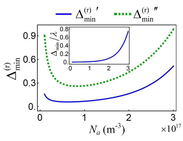
Figure 7: $\Delta_{\mathrm{min}}^{(\mathrm{r})}$ and (inset) $\Delta_{\mathrm{min}}$ versus $N_{a}$ with $\delta=2.7\gamma$ and $\theta=0.3\pi$. See text for the parameters and the others are as in Fig. 2.

The tiny shifts to be measured are easily covered by various noises, such as technical noises in the laser source, mechanical and thermal noises in the optical setups, and vacuum noises. The classical noises can be effectively suppressed by performing the experiment at RF frequency (several MHz). Thanks to the strong dependences of the shifts on the frequency of the probe beam (see Fig. 4), an RF-frequency modulation of the shifts can be easily achieved by modulating the frequency of the probe beam using, e.g. an electro-optic modulator (EOM). The output of the BHD should be measured at this modulation frequency using, e.g. an electronic spectrum analyzer (ESA). If the transmitted probe beam is assumed to be a coherent state, the signal-to-noise ratio (SNR) is given by $\mathrm{SNR}=2N_{p}\Delta^{2}/w_{0}^{2}$ Delaubert et al. (2006). The minimum measurable spatial (angular) shift is estimated as the spatial (angular) shift with $\mathrm{SNR}=1$, yielding $\Delta_{\mathrm{min}}=w_{0}/\sqrt{2N_{p}}$ Delaubert et al. (2006). Figure 7 shows, for example, the relative minimum measurable spatial (angular) shift $\Delta_{\mathrm{min}}^{(\mathrm{r})^{\prime}}=\Delta_{\mathrm{min}}/|\Delta_{y}^{\ket{y}^{\prime}}|$ ($\Delta_{\mathrm{min}}^{(\mathrm{r})^{\prime\prime}}=\Delta_{\mathrm{min}}/|\Delta_{y}^{\ket{y}^{\prime\prime}}|$) and $\Delta_{\mathrm{min}}$ (inset) as a function of $N_{a}$ with typical experimental parameters: the power of the incident probe beam $P_{p}=100\,\mu\mathrm{W}$; the beam waist of the probe beam $w_{0}=100\,\mu\mathrm{m}$; and the resolution bandwidth of the ESA $B_{\mathrm{res}}=100\,\mathrm{kHz}$. The number of the photons detected in the time interval $1/B_{\mathrm{res}}$ is $N_{p}=P_{p}e^{-2\mathrm{Im}\phi_{y}}/(B_{\mathrm{res}}\hbar\nu)$. It is clear that $\Delta_{\mathrm{min}}$ increases with $N_{a}$. However, as discussed in Sec. III, $\Delta_{y}^{\ket{y}}$ is enhanced with a large $N_{a}$ [see Fig. 5 (a)]. The optimal $N_{a}$ is obtained when $\Delta_{\mathrm{min}}^{(\mathrm{r})^{\prime}}$ and $\Delta_{\mathrm{min}}^{(\mathrm{r})^{\prime\prime}}$ are minimum. For the present parameters, the optimal $N_{a}$ is about $1\times 10^{17}\,\mathrm{m}^{-3}$, and the minimum measurable spatial and angualr shifts angle are then estimated to be $\Delta_{\mathrm{min}}\approx 9.0\,\mathrm{nm}$ and $\Delta_{\mathrm{min}}/z_{\mathrm{R}}\approx 0.23\,\mu\mathrm{rad}$, respectively.

V Conclusions

We have investigated the anisotropy induced SHEL with an anisotropic EIT atomic medium. We have shown that the medium exhibits a linear birefringence in the presence of a linearly polarized coherent coupling light beam, with the optics axis along the polarization direction of the coupling beam. After passing through the medium, a linearly polarized probe light beam experiences the spin accumulation and splits into its two spin components by opposite transverse shifts. Since the SHEL shifts are tiny (at the subwavelength scale), we have further presented a flexible measurement scheme based on a BHD. The scheme allows one to measure the shifts along any direction for each spin component by appropriately choosing the polarization and transverse mode of the LO. Besides, one can measure the spatial and angular shifts independently, when the phase of the LO is chosen to be 0 and $\pi/2$, respectively. The sensitive dependence of the SHEL shifts on the frequency of the probe beam makes it possible to perform the measurement at RF frequency such that the classical noises are efficiently suppressed and the precision can reach the quantum limit. Finally, we have shown that the minimum measurable shift is estimated to be at the nanometer level under typical experimental conditions.

Appendix A Derivation of the refractive indexes

Here we derive the refractive indexes [Eq. (3) in the main text] of the atomic medium for the probe beam. We start with Maxwell’s equations for a monochromatic wave Landau et al. (2013):

$$\mathbf{B}=\frac{1}{c}\mathbf{n}\times\mathbf{E},\qquad\mathbf{D}=-\frac{1}{c\mu_{0}}\mathbf{n}\times\mathbf{B},$$ (14)

with $\mathbf{E}$ the electric field, $\mathbf{D}$ the displacement field, $\mathbf{B}$ the magnetic field, and $\mathbf{n}=c\mathbf{k}/\nu$, where the magnitude of $\mathbf{n}$, denoted by $n$, represents the refractive index. Substituting the first equation into the second equation and using $\mathbf{D}=\varepsilon_{0}\bm{\varepsilon}\cdot\mathbf{E}$ and $c=1/\sqrt{\varepsilon_{0}\mu_{0}}$, we obtain

$$n^{2}\mathbf{E}-(\mathbf{n}\cdot\mathbf{E})\mathbf{n}-\bm{\varepsilon}\cdot\mathbf{E}=0.$$ (15)

The relative permittivity $\bm{\varepsilon}$ in the coordinate frame shown in Fig. 1 (a) in the main text is

$$\bm{\varepsilon}=\left(\begin{array}[]{ccc}\varepsilon_{\sigma}\cos^{2}{\theta}+\varepsilon_{\pi}\sin^{2}{\theta}&0&(\varepsilon_{\sigma}-\varepsilon_{\pi})\sin{\theta}\cos{\theta}\\ 0&\varepsilon_{\sigma}&0\\ (\varepsilon_{\sigma}-\varepsilon_{\pi})\sin{\theta}\cos{\theta}&0&\varepsilon_{\sigma}\sin^{2}{\theta}+\varepsilon_{\pi}\cos^{2}{\theta}\end{array}\right).$$ (19)

Equation (15) is a system of homogeneous linear equations. The compatibility condition is that the determinant of its coefficient matrix vanishes. Since the probe beam propagates along the $z$-axis, $\mathbf{n}=(0,0,n)$. Substituting Eq. (19) into Eq. (15) and setting the determinant of the coefficient matrix equal to zero, we obtain

$$(n^{2}-\varepsilon_{\sigma})(n^{2}\varepsilon_{\sigma}\sin^{2}{\theta}+n^{2}\varepsilon_{\pi}\cos^{2}{\theta}-\varepsilon_{\sigma}\varepsilon_{\pi})=0,$$ (20)

and $n_{x}(\theta)$ and $n_{y}$ are two roots of $n$.

Appendix B Reduced dipole matrix elements and Rabi frequencies

The dipole moment $\mathbf{d}=\mathbf{d}_{1}+\mathbf{d}_{-1}+\mathbf{d}_{0}$ has three components $\mathbf{d}_{1}=d_{1}\hat{\mathbf{u}}_{1}^{*}$, $\mathbf{d}_{-1}=d_{-1}\hat{\mathbf{u}}_{-1}^{*}$, and $\mathbf{d}_{0}=d_{0}\hat{\mathbf{u}}_{0}^{*}$ which couple the $\sigma^{+}$, $\sigma^{-}$, and $\pi$ transitions, respectively, where $\hat{\mathbf{u}}_{0,\pm 1}$ are the spherical basis vectors with $\hat{\mathbf{u}}_{0}$ along the quantization axis. Using the Clebsch-Gordan coefficients and the Wigner-Eckart theorem, the dipole matrix element $\mathbf{d}_{f_{i+q}g_{i}(h_{i})}=d_{f_{i+q}g_{i}(h_{i})}\hat{\mathbf{u}}_{q}^{*}$ with $q=\pm 1,0$, corresponding to the transition $\ket{f,m_{F^{\prime}}=i+q}\leftrightarrow\ket{g(h),m_{F}=i}$, can be expressed as $d_{f_{i+q}g_{i}(h_{i})}=M(F^{\prime},F,m_{F},q)d$ with $d$ the reduced dipole matrix element. The factor $M$ can be found in Ref. Steck (2015). With these in hand, the factors $\kappa_{f_{i+q}g_{i}}=N_{a}|\mathbf{d}_{f_{i+q}g_{i}}|^{2}/(\varepsilon_{0}\hbar)$ in Eqs. (1) and (2) in the main text can be written as

$$\kappa_{f_{\pm 2}g_{\pm 2}} =\frac{1}{3}\kappa,\,\,\,\,\kappa_{f_{\pm 1}g_{\pm 1}}=\frac{1}{12}\kappa,$$

$$\kappa_{f_{\pm 1}g_{\pm 2}} =\kappa_{f_{\pm 2}g_{\pm 1}}=\frac{1}{6}\kappa,\,\,\,\,\kappa_{f_{0}g_{\pm 1}}=\kappa_{f_{\pm 1}g_{0}}=\frac{1}{4}\kappa,$$ (21)

with $\kappa=N_{a}d^{2}/(\varepsilon_{0}\hbar)$. The Rabi frequencies of the coupling field $\Omega_{f_{i}h_{i}}=\mathcal{E}_{c}\mathbf{d}_{f_{i}h_{i}}\cdot\hat{\bm{\epsilon}}_{c}/\hbar$ are

$$\Omega_{f_{\pm 1}h_{\pm 1}}=\frac{1}{2}\Omega,\qquad\Omega_{f_{0}h_{0}}=\frac{1}{\sqrt{3}}\Omega,$$ (22)

with $\Omega=\mathcal{E}_{c}d/\hbar$ the reduced Rabi frequency of the coupling field.

Appendix C The action of the atomic medium on arbitrary plane-wave component

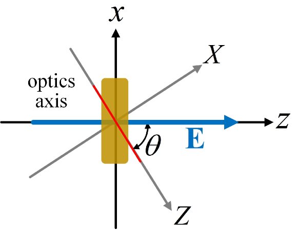
Figure 8: The coordinate frames $xyz$ and $XyZ$.

We introduce a new coordinate frame $XyZ$, which is obtained by rotating the coordinate frame $xyz$ an angle $-\theta$ around the $y$-aixs, as shown in Fig. 8. The $Z$-axis is thus along the optics axis. For each plane-wave component, one can define a local coordinate frame attached to each $\mathbf{k}=k\hat{\mathbf{k}}$ with the unit vectors $\hat{\bm{z}}_{\mathbf{k}}=\hat{\mathbf{k}}$, $\hat{\bm{y}}_{\mathbf{k}}=\hat{\bm{Z}}\times\hat{\mathbf{k}}/|\hat{\bm{Z}}\times\hat{\mathbf{k}}|$, and $\hat{\bm{x}}_{\mathbf{k}}=\hat{\bm{y}}_{\mathbf{k}}\times\hat{\mathbf{k}}$, where $\hat{\bm{Z}}$ is the unit vector along the $Z$-axis. Geometrically, $\hat{\bm{x}}_{\mathbf{k}}$ ($\hat{\bm{y}}_{\mathbf{k}}$) is parallel (perpendicular) to the plane defined by $\hat{\mathbf{k}}$ and $\hat{\bm{Z}}$. With $\hat{\mathbf{k}}=\bm{\mu}+\sqrt{1-|\bm{\mu}|^{2}}\hat{\bm{z}}\approx\mu_{x}\hat{\bm{x}}+\mu_{y}\hat{\bm{y}}+\hat{\bm{z}}$ and $\hat{\bm{Z}}=-\sin{\theta}\hat{\bm{x}}+\cos{\theta}\hat{\bm{z}}$, one has $\hat{\bm{x}}_{\mathbf{k}}\approx\hat{\bm{x}}+\mu_{y}\cot{\theta}\hat{\bm{y}}-\mu_{x}\hat{\bm{z}}$ and $\hat{\bm{y}}_{\mathbf{k}}\approx-\mu_{y}\cot{\theta}\hat{\bm{x}}+\hat{\bm{y}}-\mu_{y}\hat{\bm{z}}$. The polarization of each plane-wave component is $\hat{\bm{\epsilon}}_{\mathbf{k}}=\hat{\bm{\epsilon}}-\hat{\mathbf{k}}(\hat{\mathbf{k}}\cdot\hat{\bm{\epsilon}})$ Merano et al. (2010). For $\hat{\bm{\epsilon}}=\hat{\bm{x}}$ and $\hat{\bm{y}}$, we obtain

$$\hat{\bm{\epsilon}}_{\mathbf{k}}^{\hat{\bm{x}}} \approx\hat{\bm{x}}-\mu_{x}\hat{\bm{z}}\approx\hat{\bm{x}}_{\mathbf{k}}-\mu_{y}\cot{\theta}\hat{\bm{y}}_{\mathbf{k}}$$

$$\hat{\bm{\epsilon}}_{\mathbf{k}}^{\hat{\bm{y}}} \approx\hat{\bm{y}}-\mu_{y}\hat{\bm{z}}\approx\hat{\bm{y}}_{\mathbf{k}}+\mu_{y}\cot{\theta}\hat{\bm{x}}_{\mathbf{k}},$$ (23)

respectively. Under the action of the atomic medium, the plane-wave component with polarization $\hat{\bm{x}}_{\mathbf{k}}$ and $\hat{\bm{y}}_{\mathbf{k}}$ evolve as: $\hat{\bm{x}}_{\mathbf{k}}\rightarrow e^{i\phi_{x}(\theta+\mu_{x})}\hat{\bm{x}}_{\mathbf{k}}\approx e^{i\phi_{x}(\theta)}e^{i\mu_{x}\partial\phi_{x}(\theta)/\partial\theta}\hat{\bm{x}}_{\mathbf{k}}$ and $\hat{\bm{y}}_{\mathbf{k}}\rightarrow e^{i\phi_{y}}\hat{\bm{y}}_{\mathbf{k}}$. Therefore, $\hat{\bm{\epsilon}}_{\mathbf{k}}^{\hat{\bm{x}}}$ and $\hat{\bm{\epsilon}}_{\mathbf{k}}^{\hat{\bm{y}}}$ evolve as:

$$\hat{\bm{\epsilon}}_{\mathbf{k}}^{\hat{\bm{x}}} \rightarrow e^{i\phi_{x}(\theta)}e^{i\mu_{x}\partial\phi_{x}(\theta)/\partial\theta}\hat{\bm{x}}_{\mathbf{k}}-e^{i\phi_{y}}\mu_{y}\cot{\theta}\hat{\bm{y}}_{\mathbf{k}}$$

$$\approx e^{i\phi_{x}(\theta)}e^{i\mu_{x}\partial\phi_{x}(\theta)/\partial\theta}\left[\hat{\bm{x}}+(1-e^{-i\phi(\theta)})\mu_{y}\cot{\theta}\hat{\bm{y}}\right],$$

$$\hat{\bm{\epsilon}}_{\mathbf{k}}^{\hat{\bm{y}}} \rightarrow e^{i\phi_{y}}\hat{\bm{y}}_{\mathbf{k}}+e^{i\phi_{x}(\theta)}e^{i\mu_{x}\partial\phi_{x}(\theta)/\partial\theta}\mu_{y}\cot{\theta}\hat{\bm{x}}_{\mathbf{k}}$$

$$\approx e^{i\phi_{y}}\left[\hat{\bm{y}}-(1-e^{i\phi(\theta)})\mu_{y}\cot{\theta}\hat{\bm{x}}\right],$$ (24)

where we have ignored the $z$-components. Using the notations in the main text, we obtain

$$\ket{x} \rightarrow e^{i\phi_{x}(\theta)}e^{-i\Delta_{x}k_{x}}\left(\ket{x}+\Delta_{y}^{\ket{x}}k_{y}\ket{y}\right),$$

$$\ket{y} \rightarrow e^{i\phi_{y}}\left(\ket{y}-\Delta_{y}^{\ket{y}}k_{y}\ket{x}\right),$$ (25)

with $\Delta_{x}$, $\Delta_{y}^{\ket{x}}$, $\Delta_{y}^{\ket{y}}$ defined in the main text.

References

- Bliokh et al. (2015a) K. Yu Bliokh, F. J. Rodríguez-Fortuño, Franco Nori, and Anatoly V. Zayats, “Spin-orbit interactions of light,” Nat. Photon. 9, 796 (2015a).
- Bliokh et al. (2008a) Konstantin Y. Bliokh, Avi Niv, Vladimir Kleiner, and Erez Hasman, “Geometrodynamics of spinning light,” Nat. Photon. 2, 748 (2008a).
- Bliokh (2009) Konstantin Y. Bliokh, “Geometrodynamics of polarized light: Berry phase and spin Hall effect in a gradient-index medium,” J. Opt. A: Pure Appl. Opt. 11, 094009 (2009).
- Bliokh et al. (2015b) Konstantin Y Bliokh, Daria Smirnova, and Franco Nori, “Quantum spin Hall effect of light,” Science 348, 1448 (2015b).
- Gorodetski et al. (2012) Y. Gorodetski, K. Y. Bliokh, B. Stein, C. Genet, N. Shitrit, V. Kleiner, E. Hasman, and T. W. Ebbesen, “Weak measurements of light chirality with a plasmonic slit,” Phys. Rev. Lett. 109, 013901 (2012).
- Petersen et al. (2014) Jan Petersen, Jürgen Volz, and Arno Rauschenbeutel, “Chiral nanophotonic waveguide interface based on spin-orbit interaction of light,” Science 346, 67 (2014).
- Junge et al. (2013) Christian Junge, Danny O’Shea, Jürgen Volz, and Arno Rauschenbeutel, “Strong coupling between single atoms and nontransversal photons,” Phys. Rev. Lett. 110, 213604 (2013).
- Mitsch et al. (2014) R Mitsch, C Sayrin, B Albrecht, P Schneeweiss, and A Rauschenbeutel, “Quantum state-controlled directional spontaneous emission of photons into a nanophotonic waveguide,” Nat. Commun. 5, 5713 (2014).
- Zhao et al. (2007) Yiqiong Zhao, J. Scott Edgar, Gavin D. M. Jeffries, David McGloin, and Daniel T. Chiu, “Spin-to-orbital angular momentum conversion in a strongly focused optical beam,” Phys. Rev. Lett. 99, 073901 (2007).
- Marrucci et al. (2006) L. Marrucci, C. Manzo, and D. Paparo, “Optical spin-to-orbital angular momentum conversion in inhomogeneous anisotropic media,” Phys. Rev. Lett. 96, 163905 (2006).
- Marrucci et al. (2011) Lorenzo Marrucci, Ebrahim Karimi, Sergei Slussarenko, Bruno Piccirillo, Enrico Santamato, Eleonora Nagali, and Fabio Sciarrino, “Spin-to-orbital conversion of the angular momentum of light and its classical and quantum applications,” J. Opt. 13, 064001 (2011).
- Bliokh et al. (2011) Konstantin Y. Bliokh, Elena A. Ostrovskaya, Miguel A. Alonso, Oscar G. Rodríguez-Herrera, David Lara, and Chris Dainty, “Spin-to-orbital angular momentum conversion in focusing, scattering, and imaging systems,” Opt. Express 19, 26132 (2011).
- Sukhov et al. (2015) Sergey Sukhov, Veerachart Kajorndejnukul, Roxana Rezvani Naraghi, and Aristide Dogariu, “Dynamic consequences of optical spin–orbit interaction,” Nat. Photon. 9, 809 (2015).
- Hosten and Kwiat (2008) Onur Hosten and Paul Kwiat, “Observation of the spin Hall effect of light via weak measurements,” Science 319, 787 (2008).
- Onoda et al. (2004) Masaru Onoda, Shuichi Murakami, and Naoto Nagaosa, “Hall effect of light,” Phys. Rev. Lett. 93, 083901 (2004).
- Ling et al. (2017) Xiaohui Ling, Xinxing Zhou, Kun Huang, Yachao Liu, Cheng-Wei Qiu, Hailu Luo, and Shuangchun Wen, “Recent advances in the spin Hall effect of light,” Rep. Prog. Phys. 80, 066401 (2017).
- Haefner et al. (2009) D. Haefner, S. Sukhov, and A. Dogariu, “Spin Hall effect of light in spherical geometry,” Phys. Rev. Lett. 102, 123903 (2009).
- Aiello et al. (2009) Andrea Aiello, Norbert Lindlein, Christoph Marquardt, and Gerd Leuchs, “Transverse angular momentum and geometric spin Hall effect of light,” Phys. Rev. Lett. 103, 100401 (2009).
- Korger et al. (2014) Jan Korger, Andrea Aiello, Vanessa Chille, Peter Banzer, Christoffer Wittmann, Norbert Lindlein, Christoph Marquardt, and Gerd Leuchs, “Observation of the geometric spin Hall effect of light,” Phys. Rev. Lett. 112, 113902 (2014).
- Zhou et al. (2012a) Xinxing Zhou, Zhicheng Xiao, Hailu Luo, and Shuangchun Wen, “Experimental observation of the spin Hall effect of light on a nanometal film via weak measurements,” Phys. Rev. A 85, 043809 (2012a).
- Zhou et al. (2012b) Xinxing Zhou, Xiaohui Ling, Hailu Luo, and Shuangchun Wen, “Identifying graphene layers via spin Hall effect of light,” Appl. Phys. Lett. 101, 251602 (2012b).
- Zhu et al. (2018) Tengfeng Zhu, Yijie Lou, Yihan Zhou, Jiahao Zhang, Junyi Huang, Yan Li, Hailu Luo, Shuangchun Wen, Shiyao Zhu, Qihuang Gong, Min Qiu, and Zhichao Ruan, “Generalized spatial differentiation from spin Hall effect of light,” arXiv preprint arXiv:1804.06965 (2018).
- Bliokh (2013) A. Bliokh, K. Y. andAiello, “Goos-Hänchen and Imbert-Fedorov beam shifts: an overview,” J. Opt. 15, 014001 (2013).
- Bliokh and Bliokh (2006) Konstantin Yu. Bliokh and Yury P. Bliokh, “Conservation of angular momentum, transverse shift, and spin Hall effect in reflection and refraction of an electromagnetic wave packet,” Phys. Rev. Lett. 96, 073903 (2006).
- Bliokh et al. (2008b) Konstantin Y. Bliokh, Yuri Gorodetski, Vladimir Kleiner, and Erez Hasman, “Coriolis effect in optics: Unified geometric phase and spin-Hall effect,” Phys. Rev. Lett. 101, 030404 (2008b).
- Bomzon et al. (2002) Ze’ev Bomzon, Gabriel Biener, Vladimir Kleiner, and Erez Hasman, “Space-variant Pancharatnam–Berry phase optical elements with computer-generated subwavelength gratings,” Opt. Lett. 27, 1141 (2002).
- Shitrit et al. (2011) Nir Shitrit, Itay Bretner, Yuri Gorodetski, Vladimir Kleiner, and Erez Hasman, “Optical spin Hall effects in plasmonic chains,” Nano. Lett 11, 2038–2042 (2011).
- Bliokh et al. (2016) Konstantin Y. Bliokh, C. T. Samlan, Chandravati Prajapati, Graciana Puentes, Nirmal K. Viswanathan, and Franco Nori, “Spin-Hall effect and circular birefringence of a uniaxial crystal plate,” Optica 3, 1039 (2016).
- Fleischhauer et al. (2005) M. Fleischhauer, A. Imamoglu, and J. P. Marangos, “Electromagnetically induced transparency: Optics in coherent media,” Rev. Mod. Phys. 77, 633 (2005).
- Patnaik and Agarwal (2000) Anil K. Patnaik and G. S. Agarwal, “Laser field induced birefringence and enhancement of magneto-optical rotation,” Opt. Commun. 179, 97 (2000).
- Götte et al. (2014) Jörg B Götte, Wolfgang Löffler, and Mark R Dennis, “Eigenpolarizations for giant transverse optical beam shifts,” Phys. Rev. Lett. 112, 233901 (2014).
- Luo et al. (2011) Hailu Luo, Xinxing Zhou, Weixing Shu, Shuangchun Wen, and Dianyuan Fan, “Enhanced and switchable spin Hall effect of light near the Brewster angle on reflection,” Phys. Rev. A 84, 043806 (2011).
- Xu et al. (2016) Chenran Xu, Jingping Xu, Ge Song, Chengjie Zhu, Yaping Yang, and Girish S. Agarwal, “Enhanced displacements in reflected beams at hyperbolic metamaterials,” Opt. Express 24, 21767 (2016).
- Aharonov et al. (1988) Yakir Aharonov, David Z. Albert, and Lev Vaidman, “How the result of a measurement of a component of the spin of a spin-1/2 particle can turn out to be 100,” Phys. Rev. Lett. 60, 1351 (1988).
- Duck et al. (1989) I. M. Duck, P. M. Stevenson, and E. C. G. Sudarshan, “The sense in which a ”weak measurement” of a spin-1/2 particle’s spin component yields a value 100,” Phys. Rev. D 40, 2112 (1989).
- Ritchie et al. (1991) N. W. M. Ritchie, J. G. Story, and Randall G. Hulet, “Realization of a measurement of a ”weak value”,” Phys. Rev. Lett. 66, 1107 (1991).
- Dressel et al. (2014) Justin Dressel, Mehul Malik, Filippo M. Miatto, Andrew N. Jordan, and Robert W. Boyd, “Colloquium: Understanding quantum weak values: Basics and applications,” Rev. Mod. Phys. 86, 307 (2014).
- Dennis and Götte (2012) Mark R Dennis and Jörg B Götte, “The analogy between optical beam shifts and quantum weak measurements,” New J. Phys. 14, 073013 (2012).
- Zhou et al. (2012c) Xinxing Zhou, Hailu Luo, and Shuangchun Wen, “Weak measurements of a large spin angular splitting of light beam on reflection at the Brewster angle,” Opt. Express 20, 16003 (2012c).
- Töppel et al. (2013) Falk Töppel, Marco Ornigotti, and Andrea Aiello, “Goos–Hänchen and Imbert–Fedorov shifts from a quantum-mechanical perspective,” New. J. Phys. 15, 113059 (2013).
- Goswami et al. (2014) Sumit Goswami, Mandira Pal, Arindam Nandi, Prasanta K Panigrahi, and Nirmalya Ghosh, “Simultaneous weak value amplification of angular Goos–Hänchen and Imbert–Fedorov shifts in partial reflection,” Opt. Lett. 39, 6229 (2014).
- Hsu et al. (2004) Magnus T. L. Hsu, Vincent Delaubert, Ping Koy Lam, and Warwick P. Bowen, “Optimal optical measurement of small displacements,” J. Opt. B: Quantum Semiclass. Opt. 6, 495 (2004).
- Delaubert et al. (2006) V. Delaubert, N. Treps, M. Lassen, C. C. Harb, C. Fabre, P. K. Lam, and H-A. Bachor, “ homodyne detection as an optimal small-displacement and tilt-measurement scheme,” Phys. Rev. A 74, 053823 (2006).
- Sun et al. (2014) Hengxin Sun, Kui Liu, Zunlong Liu, Pengliang Guo, Junxiang Zhang, and Jiangrui Gao, “Small-displacement measurements using high-order Hermite-Gauss modes,” Appl. Phys. Lett. 104, 121908 (2014).
- (45) available online at http://rochesterscientific.com/ADM/.
- Cohen-Tannoudji et al. (1998) C. Cohen-Tannoudji, J. Dupont-Roc, and G. Grynberg, Atom-Photon Interactions: Basic Processes and Applications (Wiley Interscience, New York, 1998).
- Bliokh and Nori (2015) Konstantin Y. Bliokh and Franco Nori, “Transverse and longitudinal angular momenta of light,” Phys. Rep. 592, 1 (2015).
- Aiello et al. (2015) Andrea Aiello, Peter Banzer, Martin Neugebauer, and Gerd Leuchs, “From transverse angular momentum to photonic wheels,” Nat. Photon. 9, 789 (2015).
- Neugebauer et al. (2018) Martin Neugebauer, Jörg S. Eismann, Thomas Bauer, and Peter Banzer, “Magnetic and electric transverse spin density of spatially confined light,” Phys. Rev. X 8, 021042 (2018).
- Bachor and Ralph (2004) Hans-Albert Bachor and Timothy C Ralph, A guide to experiments in quantum optics (Wiley, Hoboken, 2004).
- Landau et al. (2013) L. D. Landau, E. M. Lifshitz, L. P. Pitaevskii, J. B. Sykes, J. S. Bell, and M. J. Kearsley, Electrodynamics of continuous media, Vol. 8 (Elsevier, New York, 2013).
- Steck (2015) Daniel A Steck, “Rubidium 87 D line data,” available online at http://steck.us/alkalidata (revision 2.1.5, 1/13/2015) (2015).
- Merano et al. (2010) M. Merano, N. Hermosa, J. P. Woerdman, and A. Aiello, “How orbital angular momentum affects beam shifts in optical reflection,” Phys. Rev. A 82, 023817 (2010).