Deep Information Theoretic Registration

Abstract

This paper establishes an information theoretic framework for deep metric based image registration techniques. We show an exact equivalence between maximum profile likelihood and minimization of joint entropy, an important early information theoretic registration method. We further derive deep classifier-based metrics that can be used with iterated maximum likelihood to achieve Deep Information Theoretic Registration on patches rather than pixels. This alleviates a major shortcoming of previous information theoretic registration approaches, namely the implicit pixel-wise independence assumptions. Our proposed approach does not require well-registered training data; this brings previous fully supervised deep metric registration approaches to the realm of weak supervision. We evaluate our approach on several image registration tasks and show significantly better performance compared to mutual information, specifically when images have substantially different contrasts. This work enables general-purpose registration in applications where current methods are not successful.

1 Introduction

In multi-modality image registration, mutual information (MI) and its variants have resulted in notable successes, solving many problems “out of the box” [1, 2, 3, 4]. Since these methods do not require any data beyond the images being registered, they can be referred to as “unsupervised”. Despite their strength, MI and its variants do not perform well for inter-modality image registration where, e.g., one modality has “tissue contrast” while the other has “boundary contrast” (e.g., CT to ultrasound registration). Here, a metric designed specifically for the application, such as $LC^{2}$ [5] can perform better.

Deep networks have dominated medical imaging and machine vision in the past few years, proving powerful for many applications. These networks automatically extract intermediate- and high-level representations of image structures that can be effectively used for problem solving. In view of this, might it be that deep networks could automatically learn registration metrics that perform better than those developed by human designers? Recently, registration methods based on deep networks have been developed that use classifier technology to synthesize deep metrics for registration (DMR). Simonovsky et al. [6] proposed an application specific deep metric based on Convolutional Neural Networks (CNNs). Although they showed superior performance compared to MI for deformable registration, they require well-registered training data, i.e., the method is fully supervised. Balakrishnan et al. [7] presented VoxelMorph, an unsupervised approach, where registration is modeled as a parametric function using CNNs. During training, the model parameters are optimized by maximizing image similarity which does not require ground truth registration. However, the similarity metric in VoxelMorph is designed for intra-modality registration. In another work, Hu et al. [8] described a weakly supervised approach where sparse corresponding landmarks are used to summarize the underlying dense deformation, with good results on the registration of prostate MR and ultrasound.

We propose a new approach, Deep Information Theoretic Registration (DITR), that uses Iterated Maximum Likelihood (IML) to train effective application specific deep image metrics. We show that this approach is strongly related to MI, but on patches, not pixels. This alleviates one of the main limitations of the MI approach, namely the strong implicit independence assumption on pixels or voxels. In addition, we show that in our method, neither landmarks nor well-registered training data are required for learning the deep metric. This is an important issue in some applications e.g., MRI and ultrasound, as it is not practical to perform simultaneous scanning, so that with soft tissues, accurate alignment of the training data is unlikely.

The remainder of the paper is structured as follows: Section 2 describes the relationship between Maximum Likelihood (ML) and information theoretic (IT) registration methods. In Section 3, we describe achieving ML registration using classification. Next we demonstrate that the need for accurately registered training data is relaxed by using IML with deep classifier technology. Finally, in Section 4 we evaluate our proposed method for multi-modality image registration, and explore data augmentation techniques that also help to obviate the need for accurately registered training data.

2 Maximum Likelihood Registration

Before introducing the relation between deep image metrics and MI registration, we provide a brief history of ML and MI based registration methods. Given that ML is older than IT, it is perhaps interesting that ML registration appeared after MI, in [9]. We write ML registration of a fixed image $U$ and moving image $V$ as

$$\hat{\beta}=\operatorname*{\arg\!\max}_{\beta}\ln p(U,V;\beta,\hat{\theta})=\operatorname*{\arg\!\max}_{\beta}\sum_{i}\ln p(u_{i},v_{i};\beta,\hat{\theta})~{}.$$

Here, $\beta$ are transformation parameters, and $\hat{\theta}$ are known modeling parameters, that might have been previously estimated from training data containing registered images. We also assume that the images are collections of conditionally independent features, $u_{i},v_{i}$. We model the joint distribution on model features as

$$p(u_{i},v_{i};\beta,\theta)\propto p_{R}(u_{i},{{}^{\beta}v_{i}};\theta)~{}.$$ (1)

Here, ${{}^{\beta}v}$ is shorthand for $T(v,\beta)$ where $T$ is spatial transformation applied to the feature $v$. $p_{R}(u_{i},v_{i};\theta)$ is intended as a joint distribution on features when registered. In the present work, we suppress Jacobian effects, effectively assuming that volume is approximately preserved. The parameters of this model could be estimated from training data consisting of registered images. Then,

$$\hat{\beta}=\operatorname*{\arg\!\max}_{\beta}\sum_{i}p_{R}(u_{i},{{}^{\beta}v_{i}};\hat{\theta})~{}.$$ (2)

This approach was used by Leventon et al. [9]. In that work, the features were image pixels or voxels and the joint distribution was categorical. The model was estimated by histogramming from pairs of registered images. This need for pre-registered training data is a drawback in comparison to MI.

2.1 Maximum Likelihood Registration, Unknown Parameters

To proceed without training data, we could simultaneously optimize the model parameters when registering images. If we view the model parameters as nuisance parameters, this approach has been called maximum profile likelihood  [10].

$$\widehat{\beta,\theta}=\operatorname*{\arg\!\max}_{\beta,\theta}\ln p(U,V;\beta,\theta)~{}.$$ (3)

Here Bayesians may favor averaging over the nuisance parameters. The two approaches are compared in [11]. In the context of registration, the marginalization approach was described by Zollei et al. [12]. We use the profile likelihood approach in the remainder of this paper.

2.1.1 Special Case: Registration by Minimization of Joint Entropy

We examine here the special case, as used in [9], where the features are pixels, and the model is categorical. Let the joint image intensities be discretized into bins that have a single index, calculated by the function: ${\mathcal{I}}(u_{i},v_{i})$. Suppose $u_{i},v_{i}$ are distributed according to a categorical distribution: ${\mathcal{I}}(u_{i},v_{i})|\theta\sim{\rm CAT}({\mathcal{I}}(u_{i},v_{i});\theta)$ where ${\rm CAT}(i;\theta)=\theta_{i}$, $\theta_{i}\geq 0$ , and $\sum_{i}\theta_{i}=1$. Then,

$$\hat{\beta}=\operatorname*{\arg\!\max}_{\beta}\max_{\theta}\sum_{i}\ln\theta_{{\mathcal{I}}(u_{i},{{}^{\beta}v_{i}})}=\operatorname*{\arg\!\max}_{\beta}\max_{\theta}\left[\sum_{j}N_{j}(\beta)\ln\theta_{j}\right]~{}.$$

where $i$ sums over all corresponding pairs of image intensities, $N_{j}(\beta)$ is the count of data items in bin $j$, and $j$ sums over the bins. Note that the expression in brackets is the objective function for maximum likelihood estimation of the parameters of the categorical distribution. It is easy to show, using La Grange multipliers, that the expression is maximized when $\hat{\theta_{j}}(\beta)=\frac{N_{j}(\beta)}{N}$ where $N\doteq\sum_{i}N_{i}(\beta$). Then (also dividing by $N$ inside the optimization),

$$\hat{\beta}=\operatorname*{\arg\!\max}_{\beta}\sum_{j}\frac{N_{j}(\beta)}{N}\ln\frac{N_{j}(\beta)}{N}=\operatorname*{\arg\!\min}_{\beta}{\mathds{H}\left[{\rm CAT}\left(\frac{N_{j}(\beta)}{N}\right)\right]}~{}.$$

Thus the optimization over $\beta$ has devolved exactly to minimization of joint entropy. This historically significant objective function: “adjust the registration so that the entropy of the joint histogram is minimized” [13] somewhat predates MI, they differ by marginal entropy terms that may or may not be important in practice.

2.1.2 Optimization by Coordinate Ascent

In cases where the inner optimization of Eq. 3 cannot be optimized in closed form, we may use coordinate ascent by alternating

$$\hat{\beta}^{n+1}=\operatorname*{\arg\!\max}_{\beta}\ln p(U,V,\beta,\hat{\theta^{n}})$$ (4)

and

$$\hat{\theta}^{n+1}=\operatorname*{\arg\!\max}_{\theta}\ln p(U,V,\hat{\beta^{n}},\theta)~{}.$$ (5)

Eq. 4 amounts to (re-) estimating the transformation parameters, given the (most recent) model parameter estimate. Eq. 5 re-estimates the model parameters from the (re-) registered images. We refer to this approach as “Iterated Maximum Likelihood (IML)”, it was used in Timoner’s Phd thesis [14].

2.1.3 Information-Theoretic Interpretation

Returning to the profile likelihood (Eq. 3),

$$\widehat{\beta,\theta}=\operatorname*{\arg\!\max}_{\beta,\theta}\ln p(U,V;\beta,\theta)=\operatorname*{\arg\!\max}_{\beta,\theta}\sum_{i}\ln p_{R}(u_{i},{{}^{\beta}v_{i}};\theta)~{}.$$ (6)

Considering the data to be a sample, and using the asymptotic equivalence of sample average and expectation,

$$\widehat{\beta,\theta}\approx\operatorname*{\arg\!\max}_{\beta,\theta}{\mathds{E}}_{p_{D}(u,{{}^{\beta}v})}\left[\ln p_{R}(u,{{}^{\beta}v};\theta)\right]~{},$$ (7)

where $p_{D}(u,{{}^{\beta}v})$ is the (latent) true distribution of the features in the image (after the $v$ features have been transformed). This can be re-written as

$$\hat{\beta}\approx\operatorname*{\arg\!\min}_{\beta}\left\{\min_{\theta}{\mathds{KL}}[p_{D}(u,{{}^{\beta}v})||p_{R}(u,{{}^{\beta}v};\theta)]+{\mathds{H}\left[p_{D}(u,{{}^{\beta}v})\right]}\right\}~{}.$$ (8)

In some settings, if $p_{R}$ has enough model capacity, the KL-divergence term may become unimportant, leaving only the joint entropy of the transformed data. In this case, IML converges asymptotically to the minimum joint entropy of the feature data. Similar relationships among entropy and ML (on pixels or voxels) were described in [15].

3 Maximum Likelihood Registration by Classifier

In this section, we show how to use image classification to generate an agreement metric for solving registration problems. Here a classifier is trained to distinguish between registered and unregistered patches. We use training data in form of $\{(u_{i},v_{i},z_{i})...\}$, where $u_{i}$ and $v_{i}$ are features, or patches, and $z_{i}\in\{0,1\}$. We construct the data to contain a mix of well-registered pairs of patches, labeled with $z_{i}=1$, and independently randomly uniformly unregistered pairs, $z_{i}=0$.

We construct a discriminative classifier for this problem,

$$p(z=1|u,v;\theta)\doteq\sigma(f(u,v,\theta))~{},$$ (9)

where $\sigma(\cdot)$ is the sigmoid function, $f(\cdot)\in R$, and $\theta$ represents the model parameters. $f(\cdot)$ can be any probabilistic classifier including a deep network. We use ML to train the conditional model (this is also called minimum cross entropy in the deep learning community).

$$\hat{\theta}=\operatorname*{\arg\!\max}_{\theta}\sum_{i}\ln p(z_{i}|u_{i},v_{i};\theta)~{}.$$

Next, we construct a joint distribution on registered patches that is based on the classifier. From Bayes’ rule, and noting that $z_{i}$ does not depend on the parameters,

$$p(u_{i},v_{i}|z_{i};\theta)p(z_{i})=p(z_{i}|u_{i},v_{i};\theta)p(u_{i},v_{i};\theta)~{}.$$

Taking logs and subtracting over the two cases on the value of $z_{i}$,

$$\ln p(u_{i},v_{i}|z_{i}=1;\theta)=\\[-3.50006pt] \ln p(u_{i},v_{i}|z_{i}=0;\theta)+\ln\left(\frac{p(z_{i}=1|u_{i},v_{i};\theta)}{p(z_{i}=0|u_{i},v_{i};\theta)}\right)-\ln\left(\frac{p(z_{i}=1)}{p(z_{i}=0)}\right)~{}.$$

Note that the second term on the right is the logit transform of $p(z_{i}=1|u_{i},v_{i};\theta)$, also that the logit transform is the inverse of $\sigma(\cdot)$. Then using Eq. 9, and noting that the final term is a constant,

$$\ln p(u_{i},v_{i}|z_{i}=1;\theta)=\ln(p(u_{i},v_{i}|z_{i}=0;\theta))+f(u_{i},v_{i};\theta)+C~{}.$$ (10)

For the purpose of ML registration, we construct the joint distribution on patches conditioned on a transformation with parameters $\beta$ as follows:

$$p(u_{i},v_{i};\beta,\hat{\theta})\propto p(u_{i},{{}^{\beta}v_{i}}|z_{i}=1;\hat{\theta})~{}.$$

Taking log, and using Eq. 10,

$$\ln p(u_{i},v_{i};\beta,\hat{\theta})=\ln p(u_{,}{{}^{\beta}v_{i}}|z_{i}=0)+f(u_{i},{{}^{\beta}v_{i}})+C~{}.$$

We argue that the first term on the right above is constant in $\beta$, because, in the $z_{i}=0$ case, $u_{i}$ and $v_{i}$ are independent by assumption, we further assume that $p(v_{i})$ is spatially stationary. Then, we obtain ML registration as

$$\hat{\beta}=\operatorname*{\arg\!\max}_{\beta}\sum_{i}\ln p(u_{i},v_{i};\beta,\hat{\theta})\approx\operatorname*{\arg\!\max}_{\beta}\sum_{i}f(u_{i},{{}^{\beta}v_{i}},\hat{\theta})~{}.$$ (11)

This ML objective function is simply the sum of the pre-sigmoid network responses over the corresponding patches in the pair of images being registered; it is our approach to DMR.

3.1 Unsupervised Registration by Iterated Maximum Likelihood

While DMR has proven useful, it is assumed that well-registered training data is needed. To relax this requirement, we use the IML approach of Eqns. 4 and 5; in this context the training is over features in collections of images,

$$\hat{\beta}^{n+1}=\operatorname*{\arg\!\max}_{\beta}\sum_{i}\ln p(u_{i},v_{i};\beta,\theta^{n})\approx\operatorname*{\arg\!\max}_{\beta}\sum_{i}f(u_{i},{{}^{\beta}v_{i}},\hat{\theta^{n}})\vspace{-1em}$$ (12)

and,

$$\hat{\theta}^{n+1}=\operatorname*{\arg\!\max}_{\theta}\sum_{i}\ln p(u_{i},v_{i},\hat{\beta^{n}},\theta)\approx\operatorname*{\arg\!\max}_{\theta}\sum_{i}\ln p(z_{i}|u_{,}{{}^{\hat{\beta^{n}}}v_{i}};\theta)~{}.$$ (13)

Eq. 12 amounts to estimating the transformation parameters of a collection of pairs of images using the deep metric with known model parameters, $\theta^{n}$. Eq. 13 corresponds to retraining the network using patches that are offset by the most recently estimated transformation parameters. The iteration is started with Eq. 13 on the original roughly registered training data. Subsequently, the method alternates between re-aligning the data and re-estimating the deep network parameters. In the experimental portion of the paper, three iterations are applied in training. We envision that this iterative training needs to happen only once per application type. After training, the model parameters may be fixed and used for subsequent registrations using Eq. 11.

4 Experimental Evaluation

We perform several experiments to study the effectiveness of IML approach for several image registration tasks. We introduce “dithering” as a tool to help demonstrate that the proposed approach does not require perfectly aligned training data to learn an accurate deep metric. To generate unregistered datasets, we perturb the moving images with a random transformation. We select 100 landmarks in the image space to calculate and report mean Fiducial Registration Error (FRE) following registration. We compare our method to MI, a metric used often for multi-modality image registration, as well as multi-scale MI registration (with 75 histogram bins). In all of our experiments, we use Powell’s method [16] for optimization of the transformation parameters (Eq. 12) with the learned deep metric as a cost function.

4.1 Data

We carried out experiments using the IXI Brain Development Dataset [17] which contains aligned T1-T2 image pairs from healthy subjects. In our experiments, we use 60 subjects for training and another 60 subjects for validation. All images are resampled to $1{\times}1{\times}1~{}mm$, and their intensity is normalized between the range of $\left[0,1\right]$. We crop 3D patches, $u_{i},v_{i}$, of size $17{\times}17{\times}17$ containing a mix of registered pairs of patches with $z_{i}=1$ (cropped from the same location in image space), and randomly uniformly unregistered pairs with $z_{i}=0$. Overall, 1 million patches are generated for each experiment.

Dithering Training a deep metric on unregistered dataset can cause bias in the response function depending on the distribution of the mis-registration in the data. For example, if the moving images were shifted in the $x$ direction, the response function will have a peak that is shifted accordingly (see Fig. 3a). Data augmentation with rotation and flipping can help reduce this bias at a cost of introducing additional variance and peaks (modes) in the response function. A smooth, single peak response function is preferred for effective optimization and learning of the transformation parameters. Traditionally, this could be remedied via image smoothing, however we show below that with DMR, smoothing is ineffective. Therefore, we propose “dithering” as an effective alternative approach to merge the multiple modes of the response function. More specifically, we deliberately introduce noise by applying 3D Gaussian distributed random displacements to the moving image prior to cropping patches $v(x_{i})\rightarrow v(x_{i}+d)$ where $d\sim N(0,\sigma^{2}I)$ and $\sigma$ is the standard deviation of the dither.

4.2 Network Architecture and Training

For learning a similarity metric for image registration, we use 3D CNNs and train the networks as discriminative classifiers to distinguish between registered and unregistered image patches in our experiments.

The architecture of our network is inspired by the 2-channel network of Zagouruko et al. [18] where patches from the fixed and moving images are the input channels of the CNN. The network has a 5-layer architecture consisting of strided 3D convolutions of size $3{\times}3{\times}3$ and ReLU activation functions followed by an average pooling layer and a sigmoid.

CNN Training and Registration We train our model by minimizing cross-entropy loss. During training, a learning rate of $5{\times}10^{-5}$, batch size of $256$ and $\ell_{2}$-regularization (weight decay) of $0.005$ is used to optimize the network. Following training, we use the sum of the pre-sigmoid network responses over the patches in the pair of images being registered as our cost function for optimization to update the transformation parameters. The process of training and transformation update may be iterated if necessary to improve registration of the training data.

4.3 Experiments

Experiment 1: Rigid and Affine Registration In this experiment, we demonstrate the effectiveness of IML approach in learning a deep metric from roughly registered pairs of images. In addition, we evaluate the contribution of dithering to registration by comparing the performance of IML with and without dithering. First, we perform a rigid registration experiment where we perturb the moving images by applying a random rigid transformation with parameters sampled from a 3D uniform distribution of $\mathcal{U}_{t}\{1,25\}~{}mm$ and $\mathcal{U}_{\theta}\{0.01,0.15\}~{}rad$ for translation and rotation, respectively. We propose 3 iterations of IML as $\text{IML}_{1}(4,100)\rightarrow\text{IML}_{2}(2,15)\rightarrow\text{IML}_{3}(0,0)$ where $\text{IML}(l,\sigma^{2})$ represents training a model with images that are donwnsampled by factor of $l$ and moving images dithered with a variance of $\sigma^{2}$. Downsampling is needed because large initial mis-registrations cannot be captured by the limited patch size.

Furthermore, we experiment with affine registration to show the capability of IML in a more general registration problem. We perturb the moving images by applying a random transformation with parameters sampled from $\mathcal{U}_{t}\{1,25\}$, $\mathcal{U}_{\theta}\{0.01,0.15\}$, $\mathcal{U}_{s}\{0.95,1.05\}$ and $\mathcal{U}_{sh}\{-0.01,0.01\}$ for translation, rotation, scale and shear, respectively. We follow the 3 stage IML model proposed earlier to learn the deep metrics. We also characterize the deep metric learned from the roughly registered data as a function of translation for a test data (before perturbation), following each iteration of IML, to illustrate the nature of the objective functions.

Experiment 2: Effect of Dithering on Response Function In order to experimentally verify the value of dithering as a way to merge the modes of the response function, we compare three methods of training on data where moving images are systematically shifted $10~{}mm$ in the x direction. This is meant to simulate a situation that could occur if there were a consistent difference in setup between non-simultaneous scanning of different image modalities. These three methods are: (a) training a model on the shifted data, without any augmentation and dithering (b) training a model on the same data, with augmentation, without dithering, and (c) training a model on the same data, with augmentation and dithering. In another experiment, to compare dithering and smoothing for broadening the response function, we perform an experiment in which we learn a deep metric on the dithered and smoothed data separately.

Experiment 3: Edge Registration We test our proposed IML approach in a more difficult multi-modality situation. More specifically, we experiment with registration of edge maps of the T1 images (extracted by the Canny edge detector) to intensities in T2 images. We apply the edge detector to the same data that was used in the rigid registration experiment, and follow 3 iterations of IML to learn the deep metric, $\text{IML}_{1}(2,20)\rightarrow\text{IML}_{2}(2,10)\rightarrow\text{IML}_{3}(0,0)$.

5 Results and Discussion

Fig. 1 shows box plots of mean FRE for different experiments performed for rigid and affine registration. Each box represents the interquartile range, and the horizontal line is the median of the distribution of mean FRE. As seen in Fig. 1a, IML with dithering performs statistically significantly better than IML without dithering (two-sided t-test $p<0.001$), and MI ($p<0.001$). Moreover, Fig. 1b demonstrates the effectiveness of IML with dithering for affine registration compared to MI ($p<0.001$). For both registration tasks, IML without dithering improves the initial registration error to some extent which further demonstrates the added value of dithering for learning deep metrics from unregistered datasets.

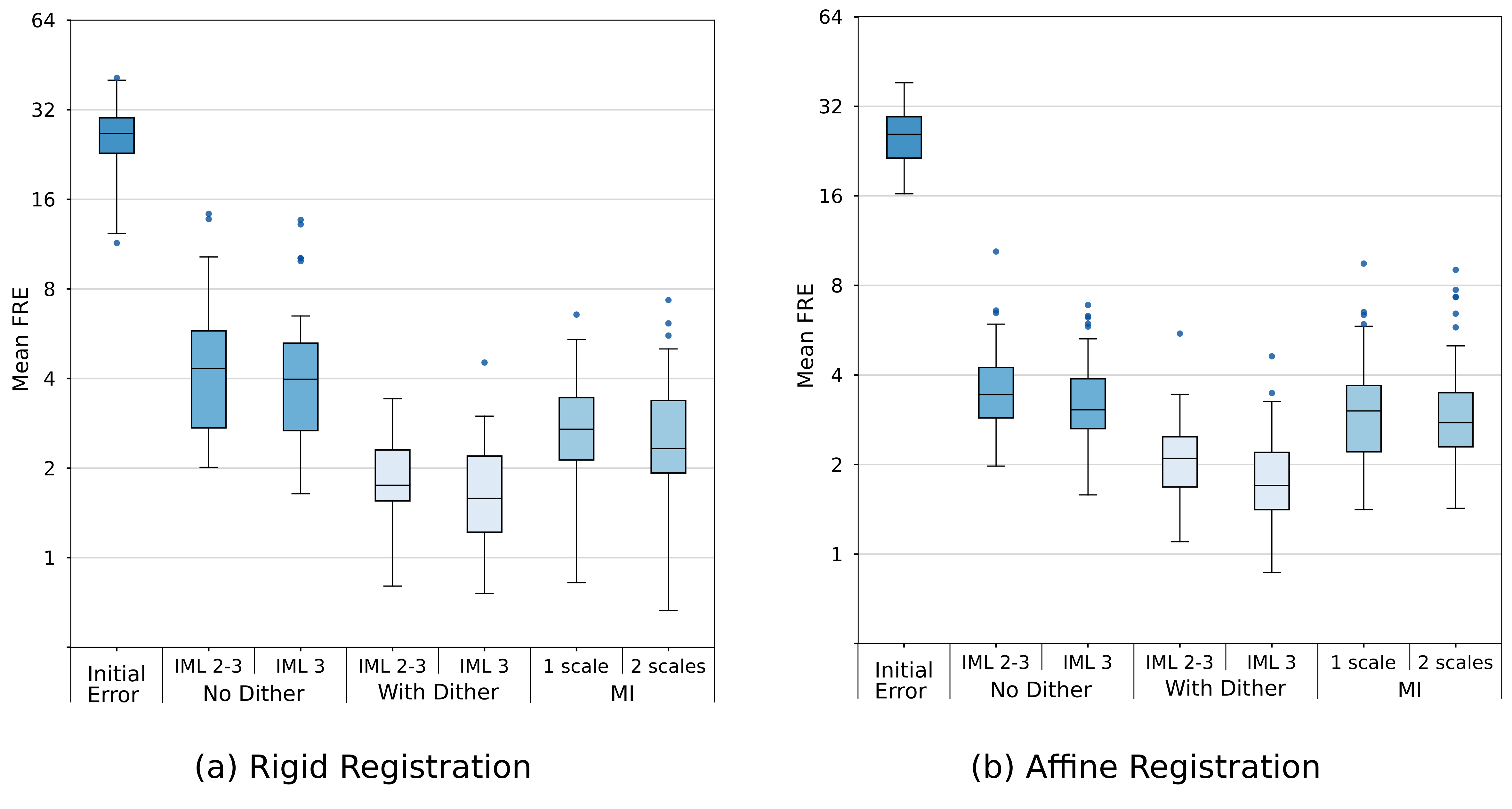
Figure 1: Box plots of mean FRE for rigid (a) and affine (b) registration between T1 and T2 images.

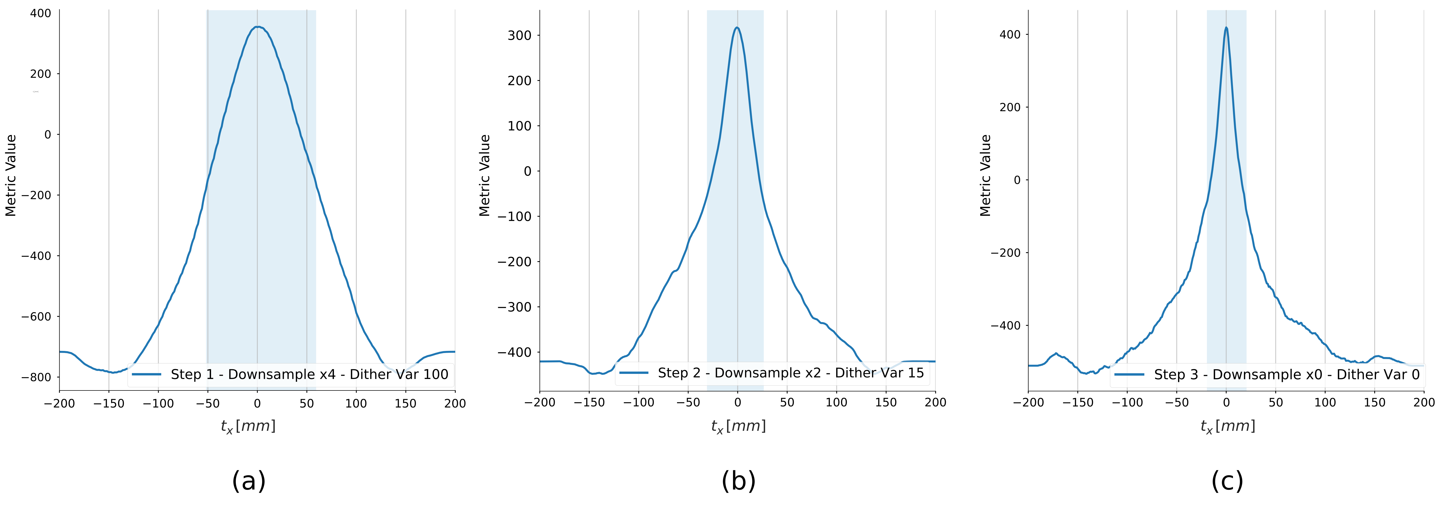
Figure 2: Response functions for each iteration of IML for rigid registration plotted as a function of translation for a pair of registered fixed and moving images. Shading illustrates full-width half max.

Fig. 2 delineates the deep metric on pairs of images as a function of translation in each iteration of IML. We observe that from the first iteration, IML(4,100), to the last iteration, the response function is sharper and hence the accuracy of the image registration improves. This is likely due to the increased level of alignment of the training data as the iterations proceed.

Fig. 3 shows the results of Experiment 2 for exploring the effect of dithering on learning deep image metrics. In Fig. 3a, it is clear that there is a bias in the response function due to the systematic shift in the training data. Fig. 3a also shows the effect of augmentation by rotation and flipping in reducing the bias. Moreover, we can see that by applying dithering to the moving image before cropping the patches, we are able to merge the peaks (modes) in the deep metric. We evaluate the impact of dithering versus smoothing on the broadness of the deep metric in Fig. 3b. It is interesting to note that smoothing has not significantly broadened the response function. We believe that deep networks are capable of effectively learning the correspondence between the smoothed patches; therefore, they can generate a sharp response similar to the response function of the deep metric learned from the original data. We see on the left that dithering is more effective at broadening the response.

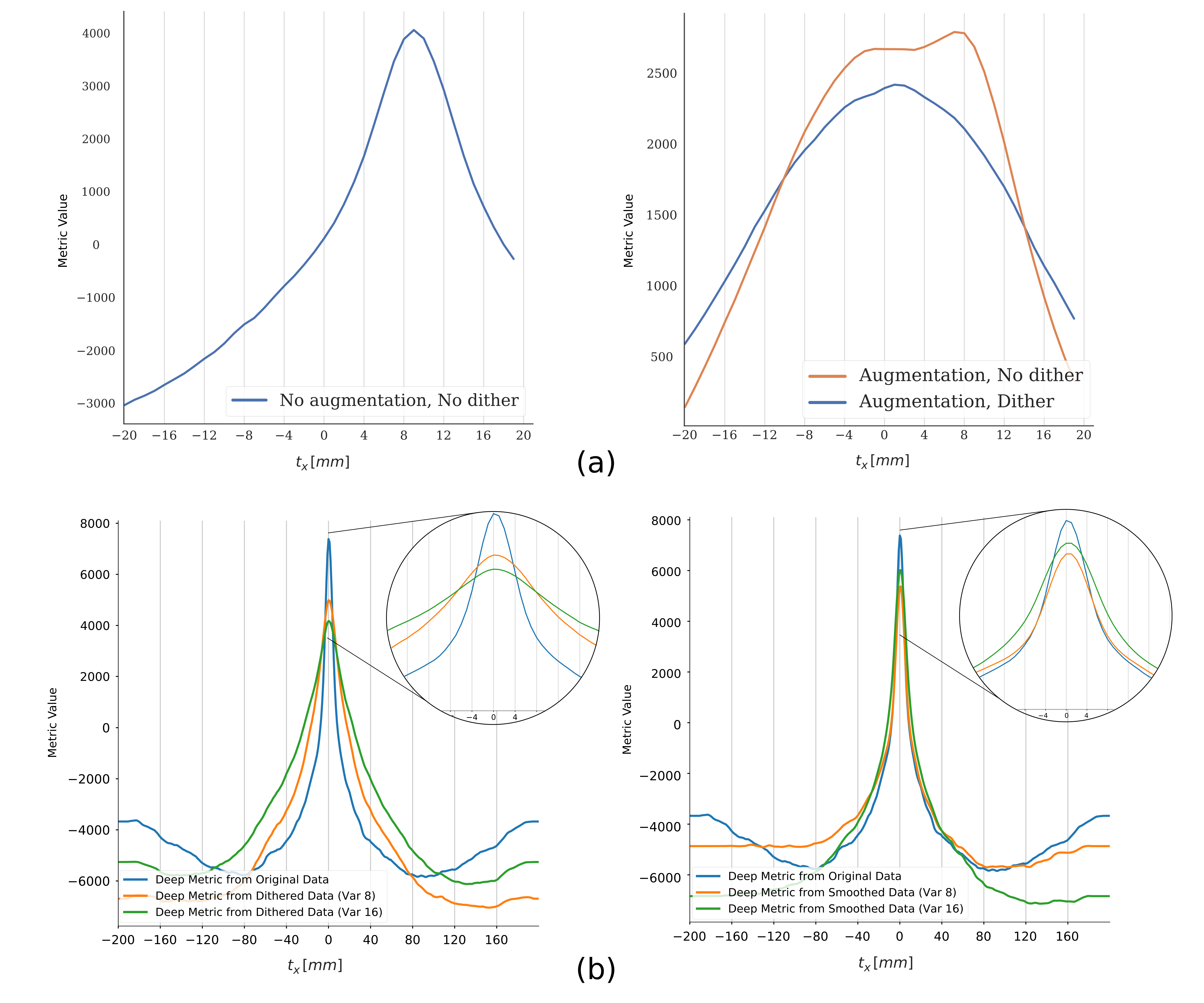
Figure 3: (a) Characteristics of the deep metric learned from different training data. (b) Impact of dithering (left) and smoothing (right) on the deep metric response function.

Fig. 4a depicts sample image pairs from the training dataset for Experiment 3, Edge Registration, with the initial mis-registration. Figure 4.b shows the mean FRE using different methods. The figure clearly demonstrates the superior performance of DITR compared to MI.

In the experiments presented, several iterations of IML are needed to learn the best deep metrics, but for registering the test data we only need the final trained network. We believe this is possible due to the broad capture range of the learned deep metric (Fig. 2).

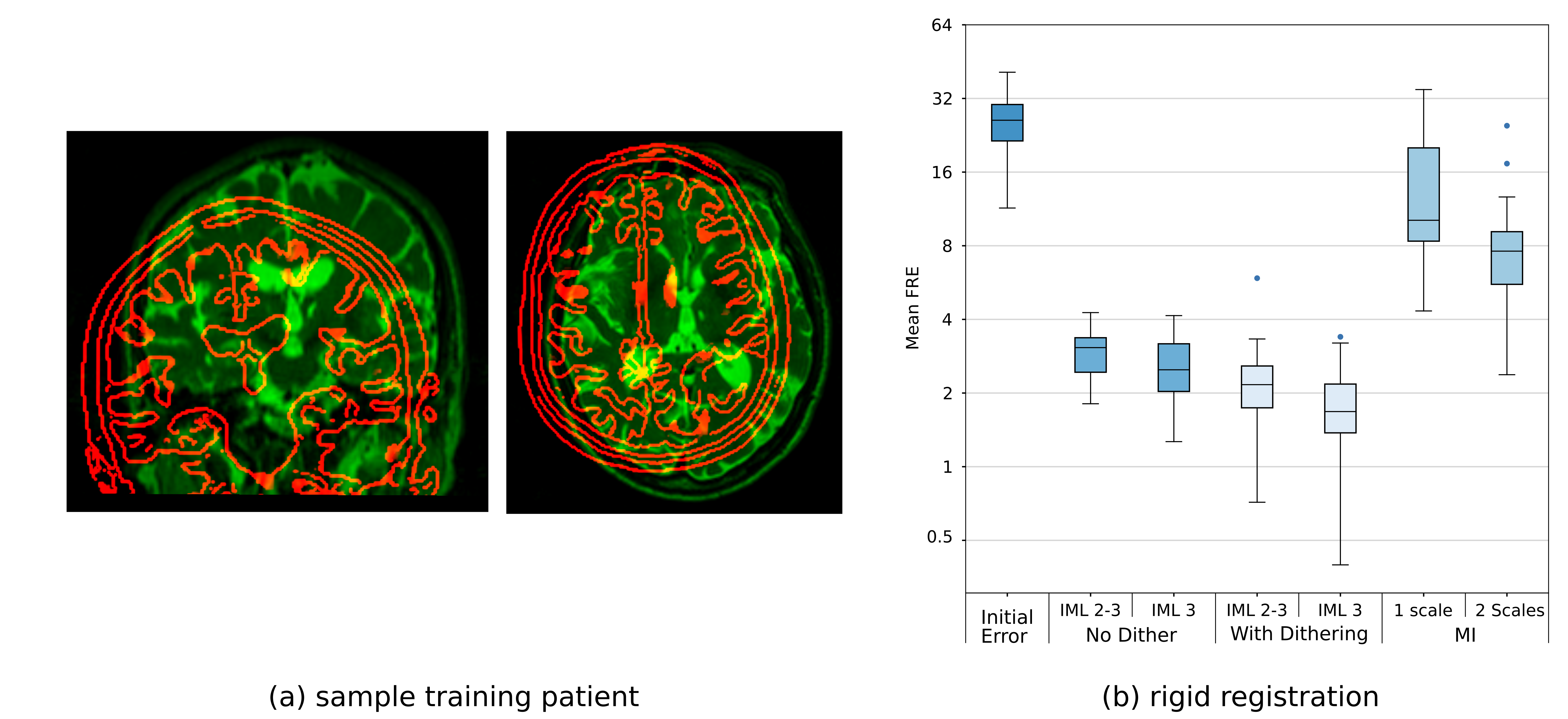
Figure 4: (a) An example case from the edge-to-image registration experiment (b) mean FRE achieved by different methods.

6 Conclusion

We presented, for the first time, an information theoretical (IT) foundation for iterated maximum likelihood (IML) registration with deep image metrics, DITR. We further showed that IML with classifier-based metrics is strongly related to mutual information on patches (not pixels).

We expect that DITR will enable new solutions for applications where the standard MI assumption of pixel- or voxel-wise independence is limiting. We demonstrated the effectiveness of our proposed method in rigid and affine registration for multi-modal data. In all experiments, DITR outperformed standard MI statistically significantly. On the edge-to-image registration experiment, MI effectively failed, but DITR successfully registered the images.

Our work focused on the analysis of registration objective functions rather than transformation modeling and optimization methods; we expect the technology to be effective in more general settings, as it is a generalization of similar DMR methods that have been shown to be successful for inter-subject deformable registration [6].

7 Acknowledgements

Research reported in this publication was supported by Natural Sciences and Engineering Research Council (NSERC) of Canada, the Canadian Institutes of Health Research (CIHR), Ontario Trillium Scholarship, NIH Grant No. P41EB015898, and NIH NIBIB Grant No. P41EB015902 Neuroimage Analysis Center.

References

- [1] William M Wells, Paul Viola, Hideki Atsumi, Shin Nakajima, and Ron Kikinis. Multi-modal volume registration by maximization of mutual information. Medical image analysis, 1(1):35–51, 1996.
- [2] Colin Studholme, Derek LG Hill, and David J Hawkes. An overlap invariant entropy measure of 3d medical image alignment. Pattern recognition, 32:71–86, 1999.
- [3] Frederik Maes, Andre Collignon, Dirk Vandermeulen, Guy Marchal, and Paul Suetens. Multimodality image registration by maximization of mutual information. IEEE transactions on Medical Imaging, 16(2):187–198, 1997.
- [4] Josien PW Pluim, JB Antoine Maintz, and Max A Viergever. Mutual-information-based registration of medical images: a survey. IEEE transactions on medical imaging, 22(8):986–1004, 2003.
- [5] Wolfgang Wein, Ali Khamene, Dirk-André Clevert, Oliver Kutter, and Nassir Navab. Simulation and fully automatic multimodal registration of medical ultrasound. In International Conference on Medical Image Computing and Computer-Assisted Intervention, pages 136–143. Springer, 2007.
- [6] Martin Simonovsky, Benjamín Gutiérrez-Becker, Diana Mateus, Nassir Navab, and Nikos Komodakis. A deep metric for multimodal registration. In International Conference on Medical Image Computing and Computer-Assisted Intervention, pages 10–18. Springer, 2016.
- [7] Guha Balakrishnan, Amy Zhao, Mert R. Sabuncu, John V. Guttag, and Adrian V. Dalca. An unsupervised learning model for deformable medical image registration. CoRR, abs/1802.02604, 2018.
- [8] Yipeng Hu, Marc Modat, Eli Gibson, Wenqi Li, Nooshin Ghavami, Ester Bonmati, Guotai Wang, Steven Bandula, Caroline M. Moore, Mark Emberton, Sébastien Ourselin, J. Alison Noble, Dean C. Barratt, and Tom Vercauteren. Weakly-supervised convolutional neural networks for multimodal image registration. Medical image analysis, 49:1–13, 2018.
- [9] Michael E Leventon and W Eric L Grimson. Multi-modal volume registration using joint intensity distributions. In International Conference on Medical Image Computing and Computer-Assisted Intervention, pages 1057–1066. Springer, 1998.
- [10] Stephen R Cole, Haitao Chu, and Sander Greenland. Maximum likelihood, profile likelihood, and penalized likelihood: a primer. American journal of epidemiology, 179 2:252–60, 2014.
- [11] Thomas A Severini. On the relationship between bayesian and non-bayesian elimination of nuisance parameters. Statistica Sinica, pages 713–724, 1999.
- [12] Lilla Zöllei, Mark Jenkinson, Samson Timoner, and William Wells. A marginalized MAP approach and EM optimization for pair-wise registration. In International Conference on Information Processing in Medical Imaging, pages 662–674, 2007.
- [13] André Collignon, Dirk Vandermeulen, Paul Suetens, and Guy Marchal. 3d multi-modality medical image registration using feature space clustering. In Computer Vision, Virtual Reality and Robotics in Medicine, pages 195–204. Springer, 1995.
- [14] Samson Timoner. Compact representations for fast nonrigid registration of medical images. 2003.
- [15] Lilla Zöllei, John W Fisher, and William M Wells. A unified statistical and information theoretic framework for multi-modal image registration. In International Conference on Information Processing in Medical Imaging, pages 366–377, 2003.
- [16] M. Powell. An efficient method for finding the minimum of a function of several variables without calculating derivatives. The Computer Journal, 7:155–162, 1964.
- [17] IXI. Information eXtraction from Images. http://brain-development.org/.
- [18] Sergey Zagoruyko and Nikos Komodakis. Learning to compare image patches via convolutional neural networks. 2015 IEEE Conference on Computer Vision and Pattern Recognition (CVPR), pages 4353–4361, 2015.