Generalized Dix equation and analytic treatment
of normal-moveout velocity for anisotropic media

Abstract

Despite the complexity of wave propagation in anisotropic media, reflection moveout on conventional common-midpoint (CMP) spreads is usually well described by the normal-moveout (NMO) velocity defined in the zero-spread limit. In their recent work, Grechka and Tsvankin showed that the azimuthal dependence of NMO velocity generally has an elliptical  shape and is determined by the spatial derivatives of the slowness vector evaluated at the CMP location. This formalism is used here to develop exact solutions for normal-moveout velocity in anisotropic media of arbitrary symmetry.

For the model of a single homogeneous layer above a dipping reflector, we obtain an explicit  NMO expression valid for all pure modes and any orientation of the CMP line with respect to the reflector strike. The influence of anisotropy on normal-moveout velocity is absorbed by the slowness components of the zero-offset ray (along with the derivatives of the vertical slowness with respect to the horizontal slownesses) – quantities that can be found in a straightforward way from the Christoffel equation. If the medium above a dipping reflector is horizontally stratified, the effective NMO velocity is determined through a Dix-type average of the matrices responsible for the “interval” NMO ellipses  in the individual layers. This generalized Dix equation provides an analytic basis for moveout inversion in vertically inhomogeneous, arbitrary anisotropic media. For models with a throughgoing vertical symmetry plane (i.e., if the dip plane of the reflector coincides with a symmetry plane of the overburden), the semi-axes of the NMO ellipse are found by the more conventional rms averaging of the interval NMO velocities  in the dip and strike directions.

Modeling of normal moveout in the most general heterogeneous anisotropic media requires dynamic ray tracing of only one (zero-offset) ray. Remarkably, the expressions for geometrical spreading along the zero-offset ray contain all the components necessary to build the NMO ellipse. This method is orders of magnitude faster than multi-azimuth, multi-offset ray tracing and, therefore, can be efficiently used in traveltime inversion and in devising fast dip-moveout (DMO) processing algorithms for anisotropic media. This algorithm becomes especially efficient if the model consists of homogeneous layers or blocks separated by smooth interfaces.

The high accuracy of our NMO expressions is illustrated by comparison with ray-traced reflection traveltimes in piecewise-homogeneous, azimuthally anisotropic models. We also apply the generalized Dix equation to field data collected over a fractured reservoir and show that $P$-wave moveout can be used to find the depth-dependent fracture orientation and evaluate the magnitude of azimuthal anisotropy.

I Introduction

Reflection moveout in inhomogeneous anisotropic media is usually calculated by multi-offset and multi-azimuth ray tracing GajewskiPsencik1987 . While the existing anisotropic ray-tracing codes are sufficiently fast for forward modeling, their application in moveout inversion requires repeated generation of azimuthally-dependent traveltimes around many common-midpoint (CMP) locations, which makes the inversion procedure extremely time-consuming. Moveout modeling, however, can be simplified by taking advantage of the limited range of offsets in conventional acquisition design. For common spreadlength-to-depth ratios close to unity, CMP traveltimes in media with moderate structural complexity are well described by the normal-moveout (NMO) velocity defined in the zero-spread limitTsvankinThomsen1994 ; GrechkaTsvankin1998 . Even if the data exhibit nonhyperbolic moveout, NMO velocity is still responsible for the most stable, small-offset portion of the moveout curve.

Existing methods for computing normal-moveout velocity in inhomogeneous media are designed for isotropic modelsShah1973 ; HubralKrey1980 . Angular velocity variations make both analytic and computational aspects of NMO-velocity modeling much more complicated. Here, we present a treatment of NMO velocity in inhomogeneous anisotropic media that provides an analytic basis for moveout inversion, leads to a dramatic increase in the efficiency of traveltime modeling methods, and helps to develop insight into the influence of the anisotropic parameters on reflection traveltimes.

Explicit expressions for normal-moveout velocity are well known for the relatively simple transversely isotropic model with a vertical symmetry axisThomsen1986 (VTI media). Recently, TsvankinTsvankin1995 presented an exact NMO equation for dipping reflectors valid in vertical symmetry planes of any homogeneous anisotropic medium. Alkhalifah and TsvankinAlkhalifahTsvankin1995 extended this result by developing a Dix-type equation for vertically inhomogeneous anisotropic media above a dipping reflector. They also showed that the NMO-velocity function in VTI media depends on just two parameters – the zero-dip NMO velocity $V_{\rm nmo}(0)$ and the “anellipticity” coefficient $\eta$. Still, their formalism is limited to 2-D wave propagation in the dip plane of the reflector, which should also coincide with a symmetry plane of the overburden.

This work is based on a general 3-D treatment of normal moveout developed by Grechka and TsvankinGrechkaTsvankin1998 , who proved that the azimuthal dependence of NMO velocity for pure (non-converted) modes has an elliptical  shape in the horizontal plane, even if the medium is arbitrary anisotropic and inhomogeneous. This conclusion breaks down only for subsurface models in which common-midpoint reflection traveltime cannot be described by a series expansion or does not increase with offset. The orientation of the NMO ellipse and the values of its semi-axes can be expressed through the spatial derivatives of the slowness vector, which are determined by both the direction of the reflector normal and the medium properties above the reflector.

Grechka and TsvankinGrechkaTsvankin1998 also presented explicit representations of the NMO velocity for a horizontal orthorhombic layer and dipping reflectors beneath VTI media. A detailed analysis of the NMO ellipse for transversely isotropic media with a horizontal symmetry axis (HTI media) is given in TsvankinTsvankin1997 , who also discusses the inversion of conventional-spread reflection moveout for the parameters of HTI media. SayersSayersSEG1995 obtained the elliptical dependence of NMO velocity for the model of a homogeneous anisotropic layer with a horizontal symmetry plane using an approximation for long-spread moveout based on group-velocity expansion in spherical harmonics.

Here, we apply the formalism of Grechka and TsvankinGrechkaTsvankin1998 to more complicated anisotropic models. We start by deriving an explicit expression for azimuthally-dependent NMO velocity from a dipping reflector overlaid by a homogeneous layer of arbitrary symmetry. Then we obtain a generalized Dix equation for NMO velocity in a model composed of a stack of horizontal homogeneous, arbitrary-anisotropic layers above a dipping reflector. While this equation has a form similar to the conventional Dix formula, it is based on the averaging of the matrices that define interval NMO ellipses. For the most general inhomogeneous media, we develop an efficient methodology to compute the normal-moveout velocity using the dynamic ray-tracing of only one (zero-offset) ray. We show that the derivatives needed to find the geometrical spreadingCervenyMolotkovPsencik1977 ; KendallThomson1989 provide sufficient information to build the NMO ellipse and, therefore, model reflection moveout without tracing a large family of rays. Finally, we compare the hyperbolic moveout equation parameterized by the exact NMO velocity with ray-traced reflection traveltimes and present a field-data application of the generalized Dix differentiation.

II Equation of the NMO ellipse

Figure 1: Normal-moveout velocity is calculated on CMP lines with different azimuths and a fixed midpoint location. It is not necessary to account for reflection-point dispersal in the derivation of NMO velocity.

Suppose the traveltimes of a certain reflected wave (reflection moveout) have been recorded on a number of common-midpoint (CMP) gathers with different azimuthal orientation but the same midpoint location (Figure 1). If the medium is anisotropic and inhomogeneous, the dependence of large-offset reflection traveltimes on the azimuth $\alpha$ of the CMP line may become rather complicated. For conventional spreadlengths close to the distance between the CMP and the reflector, however, moveout in CMP geometry is usually well-approximated by a hyperbolic equation,

$$t^{2}(\alpha)\approx t^{2}_{0}\,+\,\frac{x^{2}}{V^{2}_{\rm nmo}\,(\alpha)}\,.$$ (1)

Here $t_{0}$ is the zero-offset reflection time, $x$ is the source-receiver offset, and $V_{\rm nmo}\,(\alpha)$ is the normal-moveout velocity defined as

$$V_{\rm nmo}^{2}\,(\alpha)=\lim_{x\rightarrow 0}\,{d[x^{2}]\over d[t^{2}(\alpha)]}\,.$$ (2)

The analysis below is based on the general result of Grechka and TsvankinGrechkaTsvankin1998 , who showed that NMO velocity is described by the following simple quadratic form:

$$V_{\rm nmo}^{-2}(\alpha)=W_{11}\cos^{2}\alpha+2\,W_{12}\sin\alpha\cos\alpha+W_{22}\sin^{2}\alpha\,,$$ (3)

where ${\bf W}$ is a symmetric matrix defined as

$$W_{ij}=\tau_{0}\,{{\partial^{2}\tau}\over{\partial x_{i}\partial x_{j}}}\Biggl{|}_{\bf x_{\rm CMP}}=\tau_{0}\,{{\partial p_{i}}\over{\partial x_{j}}}\Biggl{|}_{\bf x_{\rm CMP}},\quad(i,j=1,2)\,.$$ (4)

Here, $\tau(x_{1},\,x_{2})$ is the one-way traveltime from the zero-offset reflection point to the location ${\bf x}\,\{x_{1},\,x_{2}\}$ at the surface, $\tau_{0}$ is the one-way zero-offset traveltime, $p_{i}$ are the components of the slowness vector corresponding to the ray emerging at the point x, and ${\bf x_{\rm CMP}}$ corresponds to the CMP location; the origin of the coordinate system in the derivations below coincides with the zero-offset reflection point. The one-way traveltimes appear in equation (4) because reflection-point dispersal has no influence on the NMO velocity of pure modes, and (for the small source-receiver offsets appropriate for estimation of $V_{\rm nmo}$) rays can be assumed to propagate through the reflection point of the zero-offset rayHubralKrey1980 ; Tsvankin1995 .

It is convenient to use the eigenvectors of the matrix W as auxiliary horizontal axes and rotate the NMO equation (3) by the angle $\beta$ (see Appendix A),

$$\beta=\tan^{-1}\left[\frac{W_{22}-W_{11}+\sqrt{(W_{22}-W_{11})^{2}+4W_{12}^{2}}}{2W_{12}}\right].$$ (5)

This rotation transforms equation (3) into

$$V_{\rm nmo}^{-2}(\alpha)=\lambda_{1}\cos^{2}(\alpha-\beta)+\lambda_{2}\sin^{2}(\alpha-\beta)\,,$$ (6)

where $\lambda_{1,2}$ are the eigenvalues of the matrix W. Grechka and TsvankinGrechkaTsvankin1998 conclude that for positive $\lambda_{1}$ and $\lambda_{2}$ the NMO velocity (3) represents an ellipse in the horizontal plane. A negative eigenvalue implies a negative $V^{2}_{\rm nmo}$ in certain azimuthal directions and, consequently, a decrease in the CMP traveltime with offset. Although such reverse moveout can exist in some cases (e.g., for turning waves, as described by Hale et al.Haleetal1992 ), typically both $\lambda_{1}$ and $\lambda_{2}$ are positive, and the azimuthal dependence of NMO velocity is indeed elliptical. Note that this conclusion is valid for arbitrary inhomogeneous anisotropic media provided the traveltime field is sufficiently smooth to be adequately approximated by a Taylor series expansion.

III Homogeneous arbitrary anisotropic layer

III.1 General case

To obtain normal-moveout velocity for any given model from equations (3) and (4), we need to evaluate the spatial derivatives of the slowness vector at the CMP location. As demonstrated in Appendix B, for the model of a single homogeneous layer this can be done by representing the horizontal ray displacement through group velocity and using the relation between the group-velocity and slowness vectors. As a result, we find the following explicit expressions for the matrix W and azimuthally-dependent NMO velocity [equations (76) and (77)]:

$${\bf W}={{p_{1}q_{,1}+p_{2}q_{,2}-q}\over{q_{,11}q_{,22}-q_{,12}^{2}}}\,\begin{pmatrix}q_{,22}&-q_{,12}\cr-q_{,12}&q_{,11}\cr\end{pmatrix}\!,$$ (7)

$$V_{\rm nmo}^{-2}(\alpha) \equiv V_{\rm nmo}^{-2}(\alpha,p_{1},p_{2})$$ (8)

$$= {{p_{1}q_{,1}+p_{2}q_{,2}-q}\over{q_{,11}q_{,22}-q_{,12}^{2}}}\,\left[q_{,22}\cos^{2}\alpha-2q_{,12}\sin\alpha\cos\alpha+q_{,11}\sin^{2}\alpha\right],$$

where $q\equiv q(p_{1},p_{2})\equiv p_{3}$ denotes the vertical slowness component, $q_{,i}\equiv{\partial q}/{\partial p_{i}}$, and $q_{,ij}\equiv{\partial^{2}q}/{\partial p_{i}}{\partial p_{j}}$; the horizontal components of the slowness vector ($p_{1}$ and $p_{2}$) and the derivatives in equation (8) are evaluated for the zero-offset ray.

Equation (8) is valid for pure modes reflected from horizontal or dipping interfaces in media with arbitrary symmetry and any strength of the anisotropy. The normal-moveout velocity is fully determined by the azimuth $\alpha$ of the CMP line and the slowness vector of the zero-offset ray. The slowness components $p_{1}$, $p_{2}$ and $q$ can be found by solving the Christoffel equation for the slowness (phase) direction normal to the reflector. (The slowness vector of the zero-offset ray is normal to the reflecting interface at the reflection point.) Since this equation is cubic with respect to the squared phase velocity, it yields an explicit expression for the slowness vector.

The derivatives of the vertical slowness $q$ can be found directly from the Christoffel equation as well. As discussed in more detail below in the section on ray tracing, the slowness components satisfy the equation $F(q,p_{1},p_{2})=0$, where $F$ is (in general) a sixth-order polynomial with respect to $q$. For common anisotropic models with a horizontal symmetry plane (e.g., the medium can be transversely isotropic, orthorhombic or even monoclinic), $F$ becomes a cubic polynomial with respect to $q^{2}$. Hence, the derivatives $q_{,i}$ and $q_{,ij}$ can be obtained as

$$q_{,i}=-{{F_{p_{i}}}\over{F_{q}}}$$

and

$$q_{,ij}=-{{F_{p_{i}p_{j}}+F_{p_{i}q}q_{,j}+F_{p_{j}q}q_{,i}+F_{qq}q_{,i}q_{,j}}\over{F_{q}}}\,,$$ (9)

where $F_{p_{i}}\equiv{\partial F}/{\partial p_{i}}$, $F_{q}\equiv{\partial F}/{\partial q}$, $F_{p_{i}p_{j}}\equiv{\partial^{2}F}/{\partial p_{i}}{\partial p_{j}}$, $F_{p_{i}q}\equiv{\partial^{2}F}/{\partial p_{i}}{\partial q}$, and $F_{qq}\equiv{\partial^{2}F}/{\partial q^{2}}$. Therefore, all terms in equation (8) can be obtained explicitly  from the Christoffel equation.

Equation (8) can also be used to develop weak-anisotropy approximations for NMO velocity by linearizing $q$ and its derivatives in dimensionless anisotropic parameters or in perturbations in the stiffness coefficients. These analytic approximations provide valuable insight into the influence of the anisotropic parameters on normal moveoutTsvankin1995 ; Cohen1998 . There is hardly any need, however, to substitute weak-anisotropy approximations for the exact equations in numerical modeling.

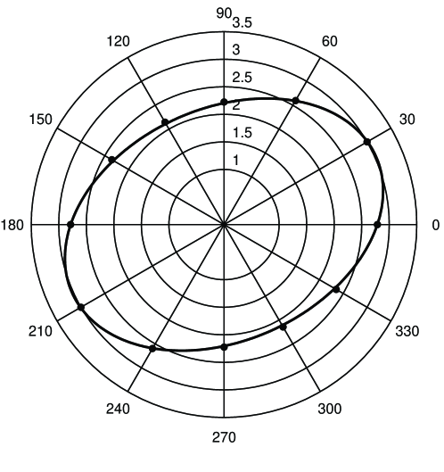
Figure 2: Comparison of the $P$-wave NMO velocity from equation (8) (solid line) and the moveout (stacking) velocity (dots) obtained by least-squares fitting of a hyperbola to the exact traveltimes computed for spreadlength equal to the distance between the CMP and the reflector. The model contains a homogeneous orthorhombic layer (with the vertical symmetry planes at azimuths 0^∘ and 90^∘) above a plane dipping reflector; the dip and azimuth of the reflector are equal to 30^∘ (azimuthal angles are shown along the perimeter of the plot). The relevant medium parameters [in Tsvankin’sTsvankin1997 notation] are $V_{P0}=2.0$ km/s, $\epsilon^{\rm(1)}=0.110$, $\delta^{\rm(1)}=-0.035$, $\epsilon^{\rm(2)}=0.225$, $\delta^{\rm(2)}=0.100$, $\delta^{\rm(3)}=0$. The vertical symmetry plane at zero azimuth has the properties of the VTI model of Dog Creek shale, while the second vertical symmetry plane is equivalent to Taylor sandstone; both models are described in ThomsenThomsen1986 .

Thus, equation (8) gives a simple and numerically efficient recipe to obtain azimuthally-dependent reflection moveout in an arbitrary anisotropic layer. The example in Figure 2, generated for an orthorhombic layer above a dipping reflector, illustrates the high accuracy of the hyperbolic moveout equation parameterized by the analytic NMO velocity (8) in describing conventional-spread reflection traveltimes. Despite the presence of anisotropy-induced nonhyperbolic moveout, the $P$-wave NMO velocity is close to the moveout (stacking) velocity calculated from the exact traveltimes on six CMP lines with different orientation. The maximum difference between $V_{\rm nmo}$ (solid line) and the finite-spread moveout velocity (dots) is just 1.4%, which is even less than the corresponding value (2.7%) for the same model, but with a horizontal reflectorGrechkaTsvankin1998 . Therefore, the magnitude of nonhyperbolic moveout for this model decreases with reflector dip; the same observation was made by TsvankinTsvankin1995 for vertical transverse isotropy. Note that although the azimuth of the dip plane of the reflector is equal to 30^∘, the largest axis of the $V_{\rm nmo}(\alpha)$ ellipse has an azimuth of 24.3^∘ due to the influence of the azimuthal anisotropy above the reflector.

III.2 Special cases

III.2.1 Model with a vertical symmetry plane

Next, let us consider a special case – a model in which the dip plane of the reflector coincides with a vertical symmetry plane of the layer. The medium can be, for instance, transversely isotropic with the symmetry axis confined to the dip plane or orthorhombic. The mirror symmetry with respect to the dip plane implies that one of the axes of the NMO ellipse points in the dip direction. Below, we provide a formal proof of this fact, as well as concise expressions for the azimuthally dependent NMO velocity in this model.

It is convenient to align the $x_{1}$-axis with the azimuth of the dip plane, while the $x_{2}$-axis will point in the strike direction. Evidently, the zero-offset ray should lie in the vertical symmetry plane $x_{2}=0$, and its slowness component $p_{2}$ goes to zero. As another consequence of the mirror symmetry with respect to the dip plane, $\partial p_{2}/\partial x_{1}=0$ (i.e, rays corresponding to $x_{2}=0$ stay in the dip plane and cannot have a non-zero $p_{2}$), so the cross-term $q_{,12}$ in equation (8) vanishes, and the NMO velocity simplifies to

$$V_{\rm nmo}^{-2}(\alpha,p_{1})={{p_{1}q_{,1}-q}\over{q_{,11}q_{,22}}}\,\left[q_{,22}\cos^{2}\alpha+q_{,11}\sin^{2}\alpha\right]\!.$$ (10)

Equation (10) describes an ellipse with the semi-axes in the dip ($\alpha=0$) and strike ($\alpha=\pi/2$) directions:

$$V_{\rm nmo}^{2}(\alpha=0,\,p_{1})={{q_{,11}}\over{p_{1}q_{,1}-q}}\,,$$ (11)

$$V_{\rm nmo}^{2}(\alpha={\pi\over 2},\,p_{1})={{q_{,22}}\over{p_{1}q_{,1}-q}}\,.$$ (12)

The dip-line NMO velocity (11) was originally obtained via the in-plane phase velocity $V$ by TsvankinTsvankin1995 :

$$V_{\rm nmo}(0,\phi)=\frac{V(\phi)}{\cos\phi}\,\dfrac{\sqrt{1+\left.\dfrac{1}{V(\phi)}\dfrac{d^{2}V}{d\theta^{2}}\right|_{\,\theta=\phi}}}{1-\left.\dfrac{\tan\phi}{V(\phi)}\,\dfrac{dV}{d\theta}\right|_{\,\theta=\phi}}\,,$$ (13)

where $\theta$ is the phase angle with vertical in the dip plane, and $\phi$ is the reflector dip. In the form (11) $V_{\rm nmo}^{2}(0,p_{1})$ was first given by CohenCohen1998 . Equation (12) provides a similar representation for the NMO velocity in the strike direction.

Equations (11) and (12) are always valid for transversely isotropic media with a vertical symmetry axis because of the mirror symmetry with respect to any vertical plane in this model. The vertical slowness in VTI media can be represented as $q(p_{1},p_{2})\equiv q\!\left(\!\sqrt{p_{1}^{2}+p_{2}^{2}}\right)$ and, for $p_{2}=0$, $q_{,22}=q_{,1}/p_{1}$. Then equation (12) for the strike-line NMO velocity reduces to the expression obtained previouslyGrechkaTsvankin1998 ,

$$V_{\rm nmo}^{2}(\alpha={\pi\over 2},p_{1})={{q_{,1}}\over{p_{1}(p_{1}q_{,1}-q)}}\,.$$ (14)

Grechka and TsvankinGrechkaTsvankin1998 also gave an equivalent form of equation (14) in terms of the phase-velocity function and the weak-anisotropy approximation for $V_{\rm nmo}^{2}(\alpha={\pi\over 2},p_{1})$. Due to the axial symmetry of the VTI model, both the dip-line [equation (11)] and strike-line [equation (14)] NMO velocities depend on the derivatives of $q$ with respect to the single horizontal (in-plane) slowness component ($p_{1}$). The cubic equation for $q^{2}(p_{1})$ in VTI media is particularly easy to solve because it splits into a quadratic equation for $P-SV$ waves and a linear equation for the $SH$-wave.

Finally, in isotropic media the vertical slowness can be directly expressed through the reflector dip $\phi$:

$$q=\sqrt{V^{-2}-p_{1}^{2}}={\cos\phi\over V}\,,$$

and equations (13) and (14) yield the well-known relationships presented by LevinLevin1971 :

$$V_{\rm nmo}(\alpha=0)={V\over{\cos\phi}}\,,$$ (15)

$$V_{\rm nmo}(\alpha={\pi\over 2})=V\,.$$ (16)

III.2.2 Horizontal reflector

For a horizontal reflector ($p_{1}=p_{2}=0$), equation (8) reduces to

$$V_{\rm nmo}^{-2}(\alpha,0,0)=-\,{{q}\over{q_{,11}q_{,22}-q_{,12}^{2}}}\,\left[q_{,22}\cos^{2}\alpha-2q_{,12}\sin\alpha\cos\alpha+q_{,11}\sin^{2}\alpha\right],$$ (17)

where $q$ and $q_{,ij}$ should be evaluated at the vertical slowness direction.

Further simplification can be achieved for a medium with a vertical symmetry plane. Aligning the $x_{1}$-axis with the symmetry-plane direction and substituting $p_{1}=0$ into equation (10) [or $q_{,12}=0$ into equation (17)] yields

$$V_{\rm nmo}^{-2}(\alpha)=-\,{{q}\over{q_{,11}q_{,22}}}\,\left[q_{,22}\cos^{2}\alpha+q_{,11}\sin^{2}\alpha\right].$$ (18)

As shown by Grechka and TsvankinGrechkaTsvankin1998 , for an orthorhombic layer (that has two mutually orthogonal symmetry planes) $P$-wave NMO velocity from equation (18) becomes a simple function of the vertical $P$-wave velocity $V_{P0}$ and the anisotropic coefficients $\delta^{(1)}$ and $\delta^{(2)}$ defined by TsvankinTsvankin1997 :

$$V^{2}_{\rm nmo}(\alpha)=V^{2}_{P0}\,\frac{(1+2\delta^{(1)})\,(1+2\delta^{(2)})}{1+2\delta^{(2)}\sin^{2}\alpha+2\delta^{(1)}\cos^{2}\alpha}\,.$$ (19)

Note that the linearized $\delta$ coefficients introduced by Mensch and RasolofosaonMenschRasolofosaon1997 and Gajewski and PšenčíkGajewskiPsencik1996 within the framework of the weak-anisotropy approximation are not appropriate for the exact equation (19). Normal-moveout velocities for vertical and horizontal transverse isotropy can be easily found as special cases of equation (19)GrechkaTsvankin1998 . Equation (18) can also be used to derive similar expressions for the split shear waves in orthorhombic media.

IV Horizontally-layered medium above a dipping reflector

IV.1 Generalized Dix equation

Figure 3: A dipping reflector beneath a horizontally layered overburden. Normal-moveout velocity in this model can be obtained from the generalized Dix equation derived here.

Here, we show that the NMO ellipse for vertically inhomogeneous arbitrary anisotropic media above a dipping reflector (Figure 3) can be obtained by Dix-type averaging of the matrices W responsible for the interval NMO ellipses. In our derivation we essentially follow the approach employed by Alkhalifah and TsvankinAlkhalifahTsvankin1995 to obtain a “2-D” Dix-type NMO equation for rays confined to the incidence (vertical) plane that contains the CMP line. Their equation is valid only in the dip plane of the reflector, which should also coincide with a symmetry plane of the medium. In contrast, we make no assumptions about the mutual orientation of the CMP line and reflector strike, and take full account of the out-of-plane phenomena associated with both model geometry and depth-varying anisotropy.

To construct the effective NMO ellipse, we need to obtain the matrix W defined in equation (4):

$$W_{ij}(L)=\tau(L){\partial p_{i}\over\partial x_{j}(L)}\,,\quad(i,j=1,2)\,,$$ (20)

where $\tau(L)$ is the total zero-offset traveltime and $x_{i}(L)$ is the horizontal ray displacement between the zero-offset reflection point located at the $L$-th (generally dipping) interface and the surface (Figure 3). Due to the continuity of the ray, both $\tau(L)$ and $x_{i}(L)$ are equal to the sum of the respective interval values:

$$\tau(L)=\sum_{\ell=1}^{L}\tau_{\ell}\,,$$ (21)

$$x_{i}(L)=\sum_{\ell=1}^{L}x_{i,\ell}\,,\quad(i=1,2).$$ (22)

(Note that here and below in the section on layered media, the comma in the subscripts separates the layer index and does not denote differentiation.)

It is convenient to introduce an auxiliary matrix

$$Y_{ij}(L)\equiv{{\partial x_{i}(L)}\over{\partial p_{j}}}\,,\quad(i,j=1,2)$$ (23)

with derivatives evaluated for the ray parameters $p_{1}$ and $p_{2}$ of the zero-offset ray. Then

$${\bf W}\equiv{\bf W}(L)=\tau(L)\,{\bf Y}^{-1}(L)\,.$$ (24)

In a model composed of horizontally homogeneous layers above the reflector, the horizontal components $p_{1}$ and $p_{2}$ of the slowness vector remain constant along any given ray between the reflection point and the surface. Therefore, substituting equation (22) into equation (23), we find

$$Y_{ij}(L)\equiv{{\partial x_{i}(L)}\over{\partial p_{j}}}=\sum_{\ell=1}^{L}{{\partial x_{i,\ell}}\over{\partial p_{j}}}\equiv\sum_{\ell=1}^{L}Y_{ij,\ell}\,.$$ (25)

Equation (25) explains the reason for introducing the effective matrix ${\bf Y}(L)$: unlike the matrix W, it can be decomposed into the sum of the matrices ${\bf Y}_{\ell}$ for the individual layers. Since all intermediate boundaries are horizontal, the ray displacements $x_{i,\ell}$ in any layer coincide with the values that should be used in computing the matrix W and the interval NMO velocity for this particular layer. Hence, we can apply equation (24) to layer $\ell$:

$${\bf W}_{\ell}=\tau_{\ell}\,{\bf Y}_{\ell}^{-1}\,$$ (26)

and, therefore,

$${\bf Y}_{\ell}=\tau_{\ell}\,{\bf W}_{\ell}^{-1}\,.$$ (27)

Substituting equations (27) and (25) into equation (24) leads to the final result:

$${\bf W}^{-1}(L)={1\over{\tau(L)}}\,\sum_{\ell=1}^{L}\tau_{\ell}\,{\bf W}_{\ell}^{-1}\,.$$ (28)

Interval matrices ${\bf W}_{\ell}$ in terms of the components of the slowness vector are given by equation (7), while the traveltimes $\tau_{\ell}$ should be obtained from the kinematic ray tracing (i.e., by computing group velocity) of the zero-offset ray. Note that, since the eigenvalues of the matrices ${\bf W}_{\ell}$ and ${\bf W}(L)$ usually are positive (under the assumptions discussed in Grechka and TsvankinGrechkaTsvankin1998 ), these matrices are nonsingular and, therefore, can be inverted.

Equation (28) performs Dix-type averaging of the interval matrices ${\bf W}_{\ell}$ to obtain the effective matrix ${\bf W}(L)$ and the effective normal-moveout velocity $V_{\rm nmo}(\alpha,L)$. It should be emphasized that the interval NMO velocities $V_{{\rm nmo},\ell}(\alpha)$ (or the interval matrices ${\bf W}_{\ell}$) in equation (28) are computed for the horizontal components of the slowness vector of the zero-offset ray. (As follows from Snell’s law, the slowness vector of the zero-offset ray is normal to the reflector at the reflection point.) This means that the interval matrices ${\bf W}_{\ell}$ in equation (28) correspond to the generally non-existent reflectors that are orthogonal to the slowness vector of the zero-offset ray in each layer.

Rewriting equation (28) in the Dix differentiation form gives

$${\bf W}_{\ell}^{-1}={{\tau(\ell){\bf W}^{-1}(\ell)-\tau(\ell-1){\bf W}^{-1}(\ell-1)}\over{\tau(\ell)-\tau(\ell-1)}}\,.$$ (29)

Equations (28) and (29) generalize the DixDix1955 formula for horizontally-layered arbitrary anisotropic media above a dipping reflector. Formally, this extension looks relatively straightforward: the squared NMO velocities in the Dix formula are simply replaced by the inverse matrices ${\bf W}^{-1}$. Also, the generalized Dix differentiation is subject to the same limitation as its conventional counterpart: the thickness of the layer of interest (in vertical time) should not be too much smaller than the layer’s depth.

In contrast to the conventional Dix equation, however, the effective matrix ${\bf W}^{-1}(\ell-1)$ in equation (29) cannot  be obtained from seismic data directly since the corresponding reflector usually does not exist in the subsurface. Therefore, layer-stripping by means of equation (29) involves recalculating each interval matrix ${\bf W_{\ell}}$ from one value of the slowness vector (corresponding to a certain real reflector in a given layer) to another – that of the zero-offset ray. This procedure was discussed for the 2-D case by Alkhalifah and TsvankinAlkhalifahTsvankin1995 and further developed for $P$-waves in VTI media by AlkhalifahAlkhalifah1997 ; the latter paper also contains a successful application of this algorithm to field data.

Only in the simplest special case of a horizontal  reflector, does the slowness vector of the zero-offset ray not change its direction (stays vertical) all the way to the surface, and the interval matrices ${\bf W}_{\ell}$ correspond to the NMO velocities from horizontal interfaces that can be measured from reflection data. Note that although such a model is horizontally-homogeneous, the zero-offset ray is not necessarily vertical (if the medium does not have a horizontal symmetry plane), and the zero-offset reflection point may be shifted in the horizontal direction from the CMP location.

IV.2 Model with a vertical symmetry plane

Next, we consider the same special case as for the single-layer model – a medium in which all layers have a common vertical symmetry plane that coincides with the dip plane of the reflector (e.g., the symmetry is VTI). For such a model the matrices ${\bf W}_{\ell}$ in the individual layers are diagonal (see the previous section), and

$$W_{12,\ell}=0\,.$$ (30)

Consequently, the off-diagonal elements of the matrix ${\bf W}(L)$ [equation (28)] vanish as well:

$$W_{12}(L)=0\,.$$ (31)

If the matrix W is diagonal, its two components directly determine the semi-axes of the NMO ellipse [see equation (3) and Appendix A]:

$$W_{kk,\ell}=[V_{{\rm nmo},\ell}^{(k)}]^{-2}$$ (32)

and

$$W_{kk}(L)=[V_{\rm nmo}^{(k)}(L)]^{-2}\,,\quad(k=1,2)\,,$$ (33)

where [$V_{\rm nmo}^{(1)}\equiv V_{\rm nmo}(\alpha=0)$] and [$V_{\rm nmo}^{(2)}\equiv V_{\rm nmo}(\alpha={\pi/2})$] are the NMO velocities measured in the dip and strike directions, respectively.

Substitution of equations (30) – (33) into equations (28) and (29) yields more conventional Dix-type averaging and differentiation formulas for the dip- and strike-components of the normal-moveout velocity:

$$[V_{\rm nmo}^{(k)}(L)]^{2}={1\over{\tau(L)}}\sum_{\ell=1}^{L}\tau_{\ell}\,[V_{{\rm nmo},\ell}^{(k)}]^{2}$$ (34)

and

$$[V_{{\rm nmo},\ell}^{(k)}]^{2}={{\tau(\ell)[V_{\rm nmo}^{(k)}(\ell)]^{2}-\tau(\ell-1)[V_{\rm nmo}^{(k)}(\ell-1)]^{2}}\over{\tau(\ell)-\tau(\ell-1)}}\,,\quad(k=1,2)\,.$$ (35)

Equations (34) and (35) for the dip component ($k=1$) of the NMO velocity were derived by Alkhalifah and TsvankinAlkhalifahTsvankin1995 who considered 2-D wave propagation in the dip plane of the reflector. Our derivation shows that the same Dix-type equations can be applied to the strike-component ($k=2$) of the NMO velocity, which determines the second semi-axis of the NMO ellipse. Despite the close resemblance of expressions (34) and (35) to the conventional Dix equation, the interval NMO velocities in equations (34) and (35), as in the more general Dix equation discussed above, correspond to the non-existent  reflectors normal to the slowness vector of the zero-offset ray in each layer.

IV.3 Accuracy of the rms averaging of NMO velocities

Although the generalized Dix equation (28) operates with the matrices  ${\bf W}_{\ell}^{-1}$, we proved that Dix-type averaging can be applied to the dip- and strike-components of the normal-moveout velocity  in a model that has a common (throughgoing) vertical symmetry plane aligned with the dip plane of the reflector. It is also clear from the results of the previous section that the rms averaging of the interval NMO velocities is valid in any azimuthal direction, if all interval NMO ellipses degenerate into circles. Hence, the error of this more conventional averaging procedure depends on the elongation of the interval ellipses, a quantity controlled by both azimuthal anisotropy and reflector dip. In Appendix C we show that this error increases rather slowly as the interval ellipses pull away from a circle because the rms averaging of the interval velocities [equation (80)] provides a linear approximation $\tilde{V}_{\rm nmo}$ to the exact NMO velocity, if both are expanded in the “elongation” coefficient.

To quantify this conclusion, we consider two numerical examples. Figure 4 shows the azimuthally-dependent $P$-wave NMO velocity in an orthorhombic medium consisting of three horizontal layers with strong azimuthal anisotropy. While the exact NMO ellipse (solid line) happens to be close to a circle, the approximate, rms-averaged normal-moveout velocity (dashed line) has an oval noncircular shape because the interval NMO ellipses are far different from circles. The maximum error of the rms averaging is about 6.3%, which will lead to much higher errors in the interval velocities after application of the Dix differentiation (35). Evidently, for this model it is necessary to use the exact NMO equation, which properly accounts for the influence of azimuthal anisotropy on normal moveout.

For models with moderate azimuthal anisotropy and a horizontal reflector (i.e., with the interval NMO-velocity variation limited by 10-20%), the accuracy of the rms averaging of NMO velocities is much higher. This implies that for such media it is possible to obtain the interval NMO velocity by the conventional Dix differentiation at a given azimuth. In the special case of horizontally layered HTI media (transverse isotropy with a horizontal axis of symmetry), the same conclusion was made by Al-Dajani and TsvankinAlDajaniTsvankin1996 .

It should be emphasized, however, that for dipping  reflectors the Dix differentiation cannot  be applied in the standard fashion (even if the rms-averaging equation provides sufficient accuracy) because the interval NMO velocities are still calculated for non-existent reflectors and cannot be found directly from the data. In the presence of anisotropy, interval parameter estimation using dipping events is impossible without a layer-stripping procedure that requires reconstruction of the NMO ellipses in the overburden and, therefore, cannot be carried out for a single azimuth.

On the whole, we would recommend to use the generalized Dix equation for any azimuthally anisotropic model, provided the azimuthal coverage of the data is sufficient to reconstruct the dependence $V_{\rm nmo}(\alpha)$. Since our algorithm operates with the NMO ellipses rather than individual azimuthal moveout measurements, it has the additional advantage of smoothing the azimuthal variation of NMO velocity, which helps to eliminate “outliers” and stabilize the interval parameter estimation. A field-data application of the generalized Dix equation is discussed below.

Figure 4: Comparison of the exact $P$-wave NMO ellipse (solid line) and an approximate NMO velocity obtained by the Dix-type averaging [equation (80), dashed line]. The model contains three horizontal orthorhombic layers with a horizontal ($[x_{1},x_{2}]$) symmetry plane. The azimuth of the $[x_{1},x_{3}]$ symmetry plane (also, the direction of one of the axes of the interval NMO ellipse) in the first (subsurface) layer is $\beta_{1}=0^{\circ}$, in the second layer – $\beta_{2}=45^{\circ}$, and in the third layer – $\beta_{3}=60^{\circ}$. The vertical $P$-wave velocities are $V_{P0,1}=2.0$ km/s, $V_{P0,2}=3.0$ km/s, and $V_{P0,3}=3.5$ km/s; the interval zero-offset traveltimes are equal to each other ($\tau_{1}=\tau_{2}=\tau_{3}=1.0$ s). The relevant anisotropic parameters [in Tsvankin’sTsvankin1997 notation] are (subscripts denote the layer number): Layer 1 – $\delta^{\rm(1)}_{1}=0.25$, $\delta^{\rm(2)}_{1}=-0.15$, Layer 2 – $\delta^{\rm(1)}_{2}=-0.20$, $\delta^{\rm(2)}_{2}=0.20$, Layer 3 – $\delta^{\rm(1)}_{3}=0.25$, and $\delta^{\rm(2)}_{3}=-0.15$.

Another example, in which the interval NMO ellipses differ from circles due to the influence of reflector dip in a purely isotropic layered model, is shown in Figure 5. Obviously, in this model the dip plane of the reflector always represents a symmetry plane, and one of the axes of all interval NMO ellipses is parallel to the dip direction. As shown in the previous section, in this case the rms averaging of the interval NMO velocities [equations (34) or (35)] becomes exact for the dip (azimuth $\alpha=0^{\circ}$) and strike CMP lines (azimuth $\alpha=90^{\circ}$), where the interval NMO values are well knownLevin1971 . Figure 5 corroborates this conclusion: for azimuths $\alpha=0^{\circ}$ and $\alpha=90^{\circ}$ the rms-averaged NMO velocity $\tilde{V}_{\rm nmo}$ is equal to the exact value $V_{\rm nmo}$. In all other azimuths, equation (80) gives only an approximation to the exact NMO velocity. However, Figure 5 indicates that this approximation is quite accurate for small and moderate reflector dips. The maximum error of equation (80), for example, is only 0.22% for reflector dip $\phi=40^{\circ}$ and 1.85% for dip $\phi=60^{\circ}$. Clearly, the error increases with dip because the interval NMO ellipses become more elongated and diverge more from a circle.

Again, since the reflector is dipping, the interval NMO velocities in Figure 5 are calculated for the nonzero horizontal components of the slowness vector determined by the reflector dip. These interval velocities correspond to non-existent reflectors and need to be recalculated from the NMO velocities of the horizontal events (which is, however, straightforward for isotropic media).

Figure 5: The rms-averaged NMO velocity $\tilde{V}_{\rm nmo}$ normalized by the exact value in isotropic media; the azimuth is measured with respect to the dip plane of the reflector. The model contains three layers above the reflector with the interval velocities $V_{1}=2.0$ km/s, $V_{2}=3.0$ km/s, and $V_{2}=3.5$ km/s and the interval zero-offset traveltimes $\tau_{1}=\tau_{2}=\tau_{3}=1.0$ s. The reflector dips are $\phi=40^{\circ}$ (dotted line), $\phi=60^{\circ}$ (dashed-dotted), $\phi=70^{\circ}$ (dashed), and $\phi=80^{\circ}$ (solid).

V Inhomogeneous anisotropic media

V.1 Summary of ray tracing

Here, we give a brief overview of ray-theory equations for anisotropic mediaCerveny1972 ; CervenyMolotkovPsencik1977 ; KendallThomson1989 , which we use below to obtain normal-moveout velocity in the presence of both anisotropy and inhomogeneity. The wave equation can be written in the frequency domain as

$$\rho\omega^{2}u_{i}+{\partial\over{\partial x_{j}}}\left(c_{ijkl}\,{{\partial u_{l}}\over{\partial x_{k}}}\right)=0\,,$$ (36)

where $\omega$ is the angular frequency, $\rho\equiv\rho({\bf x})$ is the density, $c_{ijkl}\equiv c_{ijkl}({\bf x})=\rho({\bf x})a_{ijkl}({\bf x})$ is the elasticity tensor in the Cartesian coordinates ${\bf x}$, and ${\bf u}\equiv{\bf u}({\bf x})$ is the displacement vector. The indexes $i,j,k,l$ take on values from 1 to 3; summation over repeated indexes is implied.

Within the framework of ray theory, the displacement field is sought in the form of a series expansion,

$${\bf u}({\bf x},\omega)=\sum_{n=0}^{\infty}{{{\bf U}^{(n)}({\bf x})}\over{(-i\omega)^{n}}}\exp^{i\omega\tau({\bf x})}.$$ (37)

Substituting this trial solution into equation (36) and retaining only the leading (zeroth-order) term of the series (37) yields

$$(a_{ijkl}\,p_{j}p_{k}-\delta_{il})A_{l}=0\,,$$ (38)

where ${\bf A}\equiv{\bf U}^{(0)}$, $p_{j}\equiv p_{j}({\bf x})=\partial\tau/\partial x_{j}$ is the slowness vector, $\delta_{il}$ is the symbolic Kronecker delta, and ${\bf A}$ is the polarization vector. Note that the slowness vector $\mathbf{p}$ is normal to the wavefront $\tau({\bf x})={\rm constant}$. From equation (38) it is clear that a non-trivial (non-zero) solution for the vector ${\bf A}$ exists only if the following (Christoffel) equation is satisfied:

$$F(\mathbf{p})\equiv\det[a_{ijkl}p_{j}p_{k}-\delta_{il}]=0\,.$$ (39)

For real quantities $p_{j}$ corresponding to homogeneous waves, solutions ${\bf A}^{(r)}$ ($r=1,2,3$) of equation (38) are real and orthogonal to each other. Therefore, they can be used to form an orthonormal basis:

$${\bf A}^{(r)}\cdot{\bf A}^{(s)}=\delta_{rs}\,.$$ (40)

Since $p_{j}=\partial\tau/\partial x_{j}$ depends on ${\bf x}$ in heterogeneous media, equation (38) can be regarded as a non-linear partial differential equation for the function $\tau({\bf x})$. The Hamilton-Jacobi theory — or method of characteristics (Courant and Hilbert 1962) — can be used to rewrite this equation in the form of the ordinary differential equations (the so-called “ray” equations):

$${{dx_{m}}\over{d\tau}} = {1\over 2}\,{\partial H\over\partial{p}_{m}}=a_{imkl}A_{i}p_{k}A_{l}\,,$$

$${{dp_{m}}\over{d\tau}} = -{1\over 2}\,{\partial H\over\partial{x}_{m}}=-{1\over 2}\,{{\partial a_{ijkl}}\over{\partial x_{m}}}\,A_{i}p_{j}p_{k}A_{l}\,,\quad(m=1,2,3)\,.$$

The Hamiltonian $H$, obtained from equation (38), is given by

$$H\equiv H({\bf p},{\bf x})=a_{ijkl}A_{i}p_{j}p_{k}A_{l}=1\,.$$ (42)

Note that the first of equations (V.1) defines the group velocity,

$${\bf g}\equiv{d\mathbf{x}\over{d}\tau}\,.$$ (43)

Substituting the first equation (V.1) and equation (43) into (42), we obtain an important relation between the slowness and the group velocity vectors

$${\bf p}\cdot{\bf g}=1\,.$$ (44)

Since $\mathbf{p}=\mathbf{n}/V$, where ${\bf n}$ is the unit vector in the phase (slowness) direction, and $V$ is the phase velocity, equation (44) can be further rewritten as a relation between phase and group velocities,

$$\mathbf{n}\cdot\mathbf{g}=V\,.$$ (45)

For rays emanating from a point source located at the origin of the coordinate system, the ray-tracing equations (V.1) should be supplemented by the following initial conditions:

$$\mathbf{x}^{(0)}=\mathbf{0}\,,\qquad\mathbf{p}^{(0)}={\mathbf{n}^{(0)}\over V^{(0)}}\,.$$ (46)

The ray-tracing system (V.1) combined with the initial conditions (46) can be solved by numerical integration using, for instance, the Runge-Kutta method.

V.2 Computation of NMO velocity

The results of Grechka and TsvankinGrechkaTsvankin1998 , briefly reviewed above, show that there is no need to perform a full-scale multi-azimuth ray tracing to compute reflection traveltimes on conventional CMP spreads. It is clear from equation (3) that the NMO ellipse (6) and conventional-spread moveout as a whole are fully defined by only three quantities – $W_{11}$, $W_{12}$, and $W_{22}$. Thus, three well-separated azimuthal measurements of $V_{\rm nmo}(\alpha)$ [which usually can be obtained using hyperbolic semblance analysis based on equation (1)] are sufficient to reconstruct the NMO ellipse and find the NMO velocity for any azimuth $\alpha$. In practice, the values of $V_{\rm nmo}(\alpha)$ determined on finite CMP spreads may be distorted by the influence of nonhyperbolic moveout. However, reflection moveout (especially that of $P$-waves) for spreadlengths close to the distance of the CMP from the reflector is typically close to hyperbolic; this has been shown in a number of publicationsTsvankinThomsen1994 ; Tsvankin1995 ; GrechkaTsvankin1998 and is further illustrated by numerical examples in this work.

Although calculation of $W_{ij}$ from $V_{\rm nmo}(\alpha)$ obtained in three azimuths is much more efficient than multi-azimuth ray tracing, it still requires a considerable amount of computation and does not take advantage of the explicit expressions for the parameters of the NMO-velocity ellipse discussed above. It is much more attractive to build the NMO ellipse directly from equations (3) and (4), which requires obtaining the spatial derivatives of the ray parameter ${\partial p_{i}}/{\partial x_{j}}$ at the CMP location (i.e., for the zero-offset ray). Here, we outline an efficient method of calculating these derivatives based on the dynamic ray-tracing equations for the zero-offset ray.

Let us consider the zero-offset ray in the ray coordinates $(\gamma_{1},\gamma_{2},\tau)$. The parameter $\tau$ has the meaning of the traveltime along the ray, while $\gamma_{1}$ and $\gamma_{2}$ are supposed to uniquely determine the ray path and can be chosen, for instance, as the horizontal components of the slowness vector ($p_{1}$ and $p_{2}$). Here, we use another option suggested by KashtanKashtan1982 and Kendall and ThomsonKendallThomson1989 , and define $\gamma_{1}$ and $\gamma_{2}$ as the polar and azimuthal angles of the slowness (wave-normal) vector (respectively):

$$\mathbf{n}=(\sin\gamma_{1}\cos\gamma_{2},\sin\gamma_{1}\sin\gamma_{2},\cos\gamma_{1})\,.$$ (47)

The derivatives ${\partial p_{i}}/{\partial x_{j}}$, needed to calculate $V_{\rm nmo}(\alpha)$, can be formally written as

$${{\partial p_{i}}\over{\partial x_{j}}}={{\partial p_{i}}\over{\partial\gamma_{1}}}\,{{\partial\gamma_{1}}\over{\partial x_{j}}}+{{\partial p_{i}}\over{\partial\gamma_{2}}}\,{{\partial\gamma_{2}}\over{\partial x_{j}}}+{{\partial p_{i}}\over{\partial\tau}}\,{{\partial\tau}\over{\partial x_{j}}}\,.$$ (48)

Using the matrix notation

$${\bf P}=\left[{{\partial{\bf p}}\over{\partial\gamma_{1}}},\,{{\partial{\bf p}}\over{\partial\gamma_{2}}},\,{{\partial{\bf p}}\over{\partial\tau}}\right]\,,\qquad{\bf X}=\left[{{\partial{\bf x}}\over{\partial\gamma_{1}}},\,{{\partial{\bf x}}\over{\partial\gamma_{2}}},\,{{\partial{\bf x}}\over{\partial\tau}}\right]\,$$ (49)

and the fact that the inverse matrix ${\bf X}^{-1}$ contains the rows

$${\bf X}^{-1}=\left[\begin{array}[]{c}{\partial\gamma_{1}}/{\partial{\bf x}}\\ {\partial\gamma_{2}}/{\partial{\bf x}}\\ {\partial\tau}/{\partial{\bf x}}\end{array}\right]\,,$$

we represent equation (48) in the form

$${{\partial p_{i}}\over{\partial x_{j}}}={\bf P}\,{\bf X}^{-1}\,.$$ (50)

Hence, if the matrices (49) have been calculated for the zero-offset ray at the CMP (surface) location, the derivatives ${\partial p_{i}}/{\partial x_{j}}$, ($i,j=1,2$) can be determined as the upper-left $2\times 2$ submatrix of the $3\times 3$ matrix (50). After computing the zero-offset traveltime $\tau_{0}$ using kinematic ray tracing, we can find the NMO velocity from equations (3) and (4). Note that the values of ${\partial p_{i}}/{\partial x_{j}}$ used in the NMO-velocity calculation correspond to one-way propagation from the zero-offset reflection point to the surfaceGrechkaTsvankin1998 . In other words, both p and x should be computed for rays emanating from an imaginary source located at the reflection point of the zero-offset ray.

The third column of the matrices P and X [i.e. the derivatives ${\partial{\bf p}}/{\partial\tau}$ and ${\partial{\bf x}}/{\partial\tau}$] can be obtained using the kinematic ray-tracing equations (V.1). To find the first and second columns [i.e., the derivatives ${\partial{\bf p}}/{\partial\gamma_{n}}$ and ${\partial{\bf x}}/{\partial\gamma_{n}}$, ($n=1,2$)], let us consider the so-called dynamic ray-tracing equations responsible for the geometrical spreading along the rayCervenyMolotkovPsencik1977 ; KendallThomson1989 . These equations are obtained by differentiating the kinematic ray-tracing system (V.1) with respect to $\gamma_{1}$ and $\gamma_{2}$:

$${d\over{d\tau}}\left({{\partial x_{m}}\over{\partial\gamma_{n}}}\right) = {\partial\over{\partial\gamma_{n}}}\,\left(a_{imkl}A_{i}p_{k}A_{l}\right),$$

$${d\over{d\tau}}\left({{\partial p_{m}}\over{\partial\gamma_{n}}}\right) = -{1\over 2}\,{\partial\over{\partial\gamma_{n}}}\,\left({{\partial a_{ijkl}}\over{\partial x_{m}}}\,A_{i}p_{j}p_{k}A_{l}\right),\quad(n=1,2;\,~{}m=1,2,3)\,.$$

The initial conditions for these equations are, in turn, derived by differentiating the corresponding initial conditions (46) for the kinematic ray-tracing equations (V.1). Taking into account equation (45), we find

$${{\partial{\bf x}^{(0)}}\over{\partial\gamma_{n}}} = {\bf 0}\,,$$

$${{\partial{\bf p}^{(0)}}\over{\partial\gamma_{n}}} = {1\over V^{(0)}}\left[{{\partial{\bf n}^{(0)}}\over{\partial\gamma_{n}}}-{{\bf n}^{(0)}\over V^{(0)}}\left({\bf g}^{(0)}\cdot{{\partial{\bf n}^{(0)}}\over{\partial\gamma_{n}}}\right)\right],\quad(n=1,2)\,,$$ (52)

where $V^{(0)}$, ${\bf n}^{(0)}$, and ${\bf g}^{(0)}$ are the phase velocity, the unit vector in the wave-normal (phase) direction and the group-velocity vector at the source location. In our case, the velocities $V^{(0)}$ and ${\bf g}^{(0)}$ should be evaluated immediately above the reflector at the zero-offset reflection point (the effective source). The derivatives of the wave-normal vector ${\partial{\bf n}^{(0)}}/{\partial\gamma_{n}}$ can be computed in a straightforward way from equation (47).

Thus, the derivatives needed to obtain the normal-moveout velocity are exactly the same as those required to compute the geometrical spreading along the zero-offset ray. This result is not entirely surprising because NMO velocity is related to the wavefront curvatureShah1973 , which, in turn, determines geometrical spreading. Therefore, the azimuthally-dependent NMO velocity in inhomogeneous arbitrary anisotropic media can be computed by integrating the dynamic ray-tracing equations (V.2) for the one-way zero-offset ray and substituting the results into equations (50),  (4) and (3). Since this approach requires tracing of only one zero-offset ray together with the derivatives (V.2), it is orders of magnitude less time consuming than is the tracing of hundreds of reflected rays for different azimuths and source-receiver offsets as would otherwise be required. Moreover, as shown in the next section, our algorithm becomes significantly simpler, both analytically and computationally, if the model consists of homogeneous layers or blocks.

V.3 Piecewise homogeneous media

Let us consider a medium composed of arbitrary anisotropic homogeneous layers (or blocks) separated by smooth interfaces. In this case, the ray trajectory is piecewise linear, and integration of the kinematic ray-tracing equations (V.1) reduces to summation along straight ray segments:

$${\bf x}^{(\ell)} = {\bf x}^{(\ell-1)}+{\bf g}^{(\ell)}\,\tau^{(\ell)}\,,$$

$${\bf p}^{(\ell)} = {\rm const}\,,$$

where ${\bf x}^{(\ell-1)}$ denotes the ray coordinate at the interface between the $\ell-1$-th and $\ell$-th layer, $\tau^{(\ell)}$ is the traveltime inside the $\ell$-th layer, and $g^{(\ell)}$ is the group velocity in this layer. Differentiation of equations (V.3) yields two derivatives required in the computation of the NMO ellipse:

$${\partial{\bf x}}/{\partial\tau}={\bf g}\,,$$ (54)

$${\partial{\bf p}}/{\partial\tau}=0\,,$$ (55)

with the group-velocity vector g evaluated for the zero-offset ray at the CMP location.

To fully describe the ray path (for purposes of kinematic ray tracing), equations (V.3) must be supplemented by the boundary conditions at model interfaces for x and p. The boundary conditions will also be used in the equations for dynamic ray tracing discussed below. Since the ray has to be continuous,

$${\bf x}^{(\ell)}={\bf x}^{(\ell-1)}\,.$$ (56)

The ray parameter p satisfies Snell’s law,

$${\bf p}^{(\ell)}\times{\bf b}^{(\ell)}={\bf p}^{(\ell-1)}\times{\bf b}^{(\ell)}\,,$$ (57)

where “$\times$” denotes the cross product and ${\bf b}^{(\ell)}$ is the unit vector normal to the $\ell$-th interface at ${\bf x}^{(\ell)}$.

Integration of the dynamic ray-tracing equations (V.2) in the case of homogeneous layers is relatively straightforward as well. Continuation of the derivatives ${\partial{\bf x}}/{\partial\gamma_{n}}$ and ${\partial{\bf p}}/{\partial\gamma_{n}}$ across the $\ell$-th layer is expressed by

$${{\partial{\bf x}^{(\ell+1)}}\over{\partial\gamma_{n}}}={{\partial{\bf x}^{(\ell)}}\over{\partial\gamma_{n}}}+{{\partial{\bf g}^{(\ell+1)}}\over{\partial\gamma_{n}}}\,\tau^{(\ell+1)}$$ (58)

and

$${{\partial{\bf p}^{(\ell+1)}}\over{\partial\gamma_{n}}}={{\partial{\bf p}^{(\ell)}}\over{\partial\gamma_{n}}}\,,\quad(n=1,2)\,.$$ (59)

The derivative of the group velocity needed in equation (58) is obtained in Appendix D from equations (43) and (V.1).

To propagate the derivatives ${\partial{\bf x}}/{\partial\gamma_{n}}$ and ${\partial{\bf p}}/{\partial\gamma_{n}}$ across the $\ell$-th (smooth) interface, KashtanKashtan1982 suggested differentiating equations (56) and Snell’s law [equation (57)] with respect to $\gamma_{n}$. His results become especially simple for a plane interface with the normal ${\bf b}^{(\ell)}$:

$${{\partial{\bf x}^{(\ell)}}\over{\partial\gamma_{n}}}={{\partial{\bf x}^{(\ell-1)}}\over{\partial\gamma_{n}}}+{{\bf g}^{(\ell)}-{\bf g}^{(\ell-1)}\over{\bf g}^{(\ell-1)}\cdot{\bf b}^{(\ell)}}\>\left({\bf b}^{(\ell)}\cdot{\partial{\bf x}^{(\ell-1)}\over{\partial\gamma_{n}}}\right)$$ (60)

and

$${{\partial{\bf p}^{(\ell)}}\over{\partial\gamma_{n}}}={{\partial{\bf p}^{(\ell-1)}}\over{\partial\gamma_{n}}}-{{\bf b}^{(\ell)}\over{\bf b}^{(\ell)}\cdot{\bf g}^{(\ell)}}\>\left({\bf g}^{(\ell)}\cdot{\partial{\bf p}^{(\ell-1)}\over{\partial\gamma_{n}}}\right)\,,\quad(n=1,2)\,.$$ (61)

Equations (58) – (61) allow us to continue the initial values of the derivatives ${\partial{\bf x}}/{\partial\gamma_{n}}$ and ${\partial{\bf p}}/{\partial\gamma_{n}}$ [equations (V.2)] from the zero-offset reflection point through our layered (or blocked) model to the surface. Since the quantities needed to obtain these derivatives (i.e., the group velocity and traveltime) have to be found for the kinematic ray-tracing anyway, the additional computational cost of this operation is minimal. Finally, we calculate the derivatives ${\partial p_{i}}/{\partial x_{j}}$ from equation (50) and construct the $V_{\rm nmo}(\alpha)$ ellipse defined by equations (3) and (4).

VI Synthetic examples for inhomogeneous media

The accuracy of our single-layer NMO equation has been discussed above (see Figure 2). Here, we carry out synthetic tests to compare the hyperbolic moveout equation parameterized by the exact NMO velocity with ray-traced traveltimes for inhomogeneous anisotropic models.

Figure 7 illustrates the performance of the Dix equation (28) for a model that includes three anisotropic layers with different symmetry above a dipping reflector (Figure 6). We used ray tracing to calculate $P$-wave reflection traveltimes along six azimuths with increment $30^{\circ}$ and obtained moveout velocities (dots in Figure 7a) by fitting a hyperbola to the exact moveout. Despite the complexity of the model, the best-fit ellipse found from the finite-spread moveout velocities (dashed) are sufficiently close to the theoretical NMO ellipse (solid) computed from equations (28) and (3). A small difference between the ellipses is caused by nonhyperbolic moveout associated with both anisotropy and vertical inhomogeneity. It is clear from Figure 7b that the influence of nonhyperbolic moveout becomes substantial only at source-receiver offsets that exceed the distance between the CMP and the reflector.

Figure 6: The model used in Figure 7 to check the accuracy of the generalized Dix equation. Layer 1 is transversely isotropic with a vertical symmetry axis (VTI) and relevant parameters $V_{P0,1}=2.5$ km/s, $\epsilon_{1}=0.2$, $\delta_{1}=0.1$. Layer 2 is TI with a horizontal symmetry axis (azimuth $\beta_{2}=30^{\circ}$) and $V_{P0,2}=3.0$ km/s, $\epsilon^{\rm(V)}_{2}=-0.2$, $\delta^{\rm(V)}_{2}=-0.15$ (for HTI notation, see TsvankinTsvankinHTI1997 ). Layer 3 is orthorhombic with $V_{P0,3}=3.5$ km/s, $\epsilon^{\rm(1)}_{3}=0.2$, $\delta^{\rm(1)}_{3}=0.15$, $\epsilon^{\rm(2)}_{3}=-0.3$, $\delta^{\rm(2)}_{3}=-0.2$, $\delta^{\rm(3)}_{3}=0.05$; the azimuth of the $[x_{1},x_{3}]$ symmetry plane $\beta_{3}=60^{\circ}$. The interface depths are $z_{1}=1.0$ km, $z_{2}=2.0$ km, $z_{3}=3.0$ km. The reflector dip is $20^{\circ}$, the azimuth of the dip plane is $0^{\circ}$.

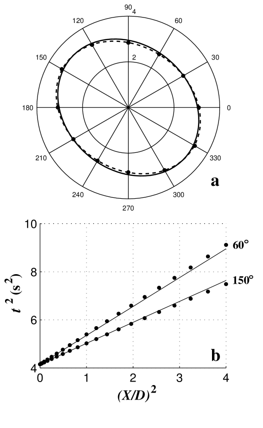
Figure 7: (a) Comparison between the theoretical $P$-wave NMO ellipse calculated from the generalized Dix equation (solid) and moveout velocities obtained from ray-traced traveltimes for spreadlength equal to the distance between the CMP and the reflector (dots). The model is shown in Figure 6; the dashed line marks the best-fit ellipse found from the finite-spread moveout velocities. (b) Hyperbolic moveout curve parameterized by the exact NMO velocity (solid) vs. computed traveltimes (dots) at azimuths $60^{\circ}$ and $150^{\circ}$; $D$ is the CMP-reflector distance.

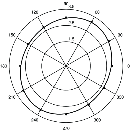
Figure 8: Comparison of the theoretical $P$-wave NMO ellipse (solid) and finite-spread moveout velocity (dots; the spreadlength is equal to the CMP-reflector distance) in an azimuthally-anisotropic model with dipping layers. The NMO ellipse is computed from equations (3) and (4), with the spatial derivatives of the ray parameter evaluated using equations (50), (54), (55), and (58) through (61). The model consists of three dipping transversely layers with different orientation of the symmetry axis. The first layer is VTI with $V_{P0,1}=2.0$ km/s, $\epsilon_{1}=0.2$, and $\delta_{1}=0.1$. The second layer is HTI with the azimuth of the symmetry axis of 30^∘ and $V_{P0,2}=2.4$ km/s, $\epsilon_{2}=0.15$, $\delta_{2}=0$. The third layer is TI with a tilted symmetry axis (the azimuth is 60^∘, the tilt is 30^∘) and $V_{P0,3}=3$ km/s, $\epsilon_{3}=0.25$, $\delta_{3}=0.08$ [for all layers we used the generic Thomsen’sThomsen1986 parameters]. The azimuth $\psi$ and dip $\phi$ of the bottom of the first layer are $\psi_{1}=70^{\circ}$ and $\phi_{1}=10^{\circ}$; for the bottom of the second layer $\psi_{2}=20^{\circ}$ and $\phi_{2}=15^{\circ}$; for the reflector $\psi_{3}=50^{\circ}$ and $\phi_{3}=35^{\circ}$. The distances between the CMP and the interfaces are 1 km, 2 km, and 3 km.

A similar example, but this time for a horizontally inhomogeneous medium above the reflector is shown in Figure 8. The model contains three transversely isotropic layers with dipping lower boundaries and differently oriented symmetry axes. The NMO ellipse (solid) provides an excellent approximation to the effective moveout velocity (dots) for all four azimuths used in the computation, with a maximum error of just about 1.4%. In addition to verifying the accuracy of our algorithm based on the evaluation of the derivatives ${\partial{\bf x}}/{\partial\gamma_{n}}$ and ${\partial{\bf p}}/{\partial\gamma_{n}}$, this test demonstrates again that the analytic (zero-spread) normal-moveout velocity typically provides a good approximation for $P$-wave reflection traveltimes on conventional spreads.

VII Field-data example

We applied the generalized Dix equation to a 3-D data set acquired by ARCO (with funding from the Gas Research Institute) in the Powder River Basin, Wyoming. A detailed description of this survey and preliminary processing results can be found in Corrigan et al.Corriganetal1996 and Withers and CorriganWithersCorrigan1997 . The main goal of the experiment was to use the azimuthal dependence of $P$-wave signatures in characterization of a fractured reservoir. Hence, the acquisition was carefully designed to provide a good offset coverage in a wide range of source-receiver azimuths. To enhance the signal-to-noise ratio, the data were collected into a number of “superbins,” each with an almost random distribution of azimuths and offsets.

Below we show the results of our velocity analysis for one of the superbins located in the southwest corner of the survey area. To obtain the azimuthal dependence of NMO velocity, we divided the traces into nine 20^∘ azimuthal sectors and carried out conventional hyperbolic semblance analysis separately for each sector. Figure 9 shows the composite CMP gather in one of the sectors with two prominent reflection events marked by arrows. According to Withers and CorriganWithersCorrigan1997 , the reflection at a two-way vertical time of 2.14 s corresponds to the bottom of the Frontier/Niobrara formations, and the event at 2.58 s is the basement reflection. Semblance panels for two sectors 100^∘ apart are displayed in Figure 10. While the best-fit stacking velocity for the event at 2.14 s is weakly dependent on azimuth, the velocity for the basement reflection is noticeably higher at azimuth N30E. This observation is confirmed by the shape of the effective NMO ellipses reconstructed from the semblance panels (Figure 11, left plot). The stacking velocity of the basement reflection along the larger semi-axis of the ellipse is 4% higher than in the orthogonal direction; the corresponding number for the shallower reflection is 1.7%. The orientation of both effective ellipses agrees with the results of Withers and CorriganWithersCorrigan1997 , who used a different algorithm. It should be mentioned that ignoring azimuthal velocity variations on the order of 3-4% and mixing up all source-receiver azimuths (as is conventionally done in 3-D processing) would inevitably lead to poor stacking and deterioration of the final seismic image.

Since the dips in the survey area are extremely smallCorriganetal1996 , the azimuthal dependence of stacking velocity can be attributed to the influence of azimuthal anisotropy associated with vertical fractures. To study the interval properties for vertical times between 2.14 and 2.58 s, we applied the generalized Dix equation (29) to the effective NMO ellipses. Note that the different orientation of the effective ellipses in Figure 11, indicative of depth-varying principal directions of the azimuthal anisotropy, does not pose a problem for the generalized Dix differentiation. The pronounced azimuthal variation in the interval NMO velocity (9%, Figure 11) can be explained by the intense fracturing in the layer immediately above the basement. The direction of the larger semi-axis of the interval NMO ellipse is in general agreement with the predominant fracture orientation in the deeper part of the section determined from borehole data and shear-wave splitting analysisWithersCorrigan1997 . Complete processing/inversion results for the survey area will be reported in forthcoming publications.

Figure 9: Common-midpoint gather composed of traces with source-receiver azimuths within a 20^∘ azimuthal sector centered at N30E.

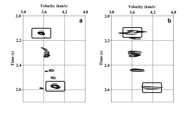
Figure 10: Semblance velocity panels for two azimuthal sectors centered at N130E (a) and N30E (b). The semblance maxima corresponding to the events at vertical times of 2.14 s and 2.58 s are framed.

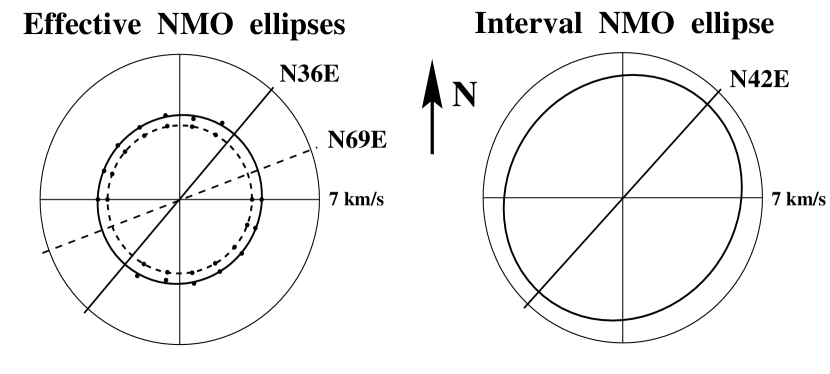
Figure 11: The effective NMO ellipses for the reflection events at 2.14 s (dashed) and 2.58 s (solid) reconstructed from the data and the corresponding interval NMO ellipse obtained by the generalized Dix differentiation. The orientation of the larger semi-axis of each ellipse is marked by a radial line.

VIII Discussion and conclusions

Azimuthally-dependent normal-moveout velocity around a certain CMP location is described by a simple quadratic form and usually has an elliptical shape, with the orientation and semi-axes of the ellipse determined by the properties of the medium and the direction of the reflector normal at the zero-offset reflection point. Using this general result obtained by Grechka and TsvankinGrechkaTsvankin1998 , we have presented a series of solutions for the exact normal-moveout velocity of pure modes in anisotropic models of various complexity. For a homogeneous anisotropic layer above a dipping reflector, NMO velocity was found explicitly as a function of the slowness vector corresponding to the zero-offset ray. This single-layer equation is valid for arbitrary anisotropic symmetry and any orientation of the CMP line with respect to the reflector strike. The vertical component of the slowness vector and its derivatives with respect to the horizontal slownesses, needed to compute the NMO velocity, can be obtained in an explicit form using the Christoffel equation. In addition to simplifying moveout modeling, our NMO equation can be effectively used in moveout inversion, as well as in developing weak-anisotropy approximations for different symmetries.

If the model contains a stack of homogeneous arbitrary anisotropic layers above a dipping reflector, the NMO ellipse should be obtained by a Dix-type averaging of the single-layer expressions described above. Instead of the squared NMO velocities in the conventional Dix formula, our generalized equation operates with the interval matrices ${\bf W}_{\ell}$ that describe the NMO ellipses  corresponding to the individual layers. To find azimuthally-dependent normal-moveout velocity, it is sufficient to compute the zero-offset traveltime and the interval NMO ellipses for the slowness vector of the zero-offset ray. The generalized Dix equation can be used to perform moveout-based interval parameter estimation in vertically inhomogeneous anisotropic models of any symmetry. It should be emphasized, however, that application of the generalized Dix differentiation to dipping events entails full-scale layer-stripping because NMO ellipses in the individual layers cannot be directly measured from the data.

One important special case considered in detail is a model with the same (throughgoing) vertical symmetry plane in all layers that also coincides with the dip plane of the reflector (e.g., the medium above the reflector is TI with a vertical symmetry axis). Because of the mirror symmetry with respect to the dip plane, the axes of the NMO ellipse are aligned with the dip and strike directions of the reflector. The generalized Dix equation in such a model reduces to the rms averaging of the dip-line and strike-line NMO velocities in the individual layers (these averages determine the semi-axes of the NMO ellipse). This result represents a 3-D extension of the Dix-type equation developed by Alkhalifah and TsvankinAlkhalifahTsvankin1995 for normal moveout in the dip plane of the reflector.

Except for this special case, the effective NMO velocity computed by the Dix rms averaging generally takes an oval anelliptic  form that thus deviates from the exact NMO ellipse. Still, this deviation is not significant if the interval NMO ellipses are close to being circles, which implies the absence of large dips and significant azimuthal anisotropy. In any case, it is preferable to apply the generalized Dix equation (as opposed to the conventional Dix differentiation at any given azimuth) for any azimuthally anisotropic model because in addition to being more accurate it also provides the important advantage of smoothing the effective moveout velocities using the correct (elliptical) functional form and thus reducing the instability in interval parameter estimation.

We complete the analysis by considering the most general inhomogeneous media and presenting an algorithm that leads to a dramatic reduction in the amount of computations needed to obtain the NMO velocity and conventional-spread reflection moveout. All information required to construct the NMO ellipse is contained in the results of the dynamic ray tracing (i.e., computation of geometrical spreading) of a single (zero-offset) ray. Although evaluation of geometrical spreading requires solving an additional system of differential equations together with the kinematic ray-tracing equations, this algorithm is orders of magnitude more efficient than multi-offset, multi-azimuth ray tracing. Furthermore, if the model consists of homogeneous layers or blocks separated by smooth interfaces, all quantities needed to find the NMO ellipse can be computed during the kinematic tracing of the zero-offset ray.

The normal-moveout velocity discussed here is defined in the zero-spread limit and cannot account for nonhyperbolic moveout caused by anisotropy and inhomogeneity on finite-spread CMP gathers. Nevertheless, our numerical examples for various anisotropic models demonstrate that the hyperbolic moveout equation parameterized by NMO velocity provides good accuracy in the description of reflection moveout (especially that of $P$-waves) on conventional spreads close to the distance between the CMP and the reflector. Even if the hyperbolic moveout approximation becomes inadequate, NMO velocity can be obtained by means of nonhyperbolic moveout analysisTsvankinThomsen1994 ; SayersSEG1995 . Hence, the results of this work can be efficiently used in traveltime inversion and dip-moveout processing for arbitrary anisotropic media.

To show the feasibility of applying our formalism in fracture detection, we processed wide-azimuth 3-D $P$-wave data acquired over a fractured reservoir in the Powder River Basin, Wyoming. The generalized Dix differentiation allowed us to obtain the depth-varying  fracture orientation and estimate the magnitude of azimuthal anisotropy (measured by $P$-wave moveout velocity). The direction of the larger semi-axis of the interval NMO ellipse in the strongly anisotropic layer above the basement is in agreement with the fracture trend in this part of the section. Therefore, if the formation of interest has a sufficient thickness, azimuthal moveout analysis of $P$-wave (and, if available, shear-wave) data by means of the generalized Dix equation provides valuable information for characterization of fracture networks.

IX Acknowledgments

We are grateful to Dennis Corrigan and Robert Withers of ARCO for providing the field data and sharing their knowledge of the processing and interpretation issues. We would like to thank Bruce Mattocks and Bob Benson (both of CSM) for helping us in data processing and Ken Larner (CSM) and Andreas Rüger (CSM; now at Landmark) for their reviews of the paper. The support for this work was provided by the members of the Consortium Project on Seismic Inverse Methods for Complex Structures at Center for Wave Phenomena, Colorado School of Mines and by the United States Department of Energy (project “Velocity Analysis, Parameter Estimation, and Constraints on Lithology for Transversely Isotropic Sediments” within the framework of the Advanced Computational Technology Initiative).

Appendix A Relation between the matrix W and the NMO-velocity ellipse

Azimuthally dependent normal-moveout velocity is described by equation (3) of the main text as a general second-order curve in the horizontal plane. The expression for $V_{\rm nmo}(\alpha)$ can be simplified further by aligning the horizontal coordinate axes with the eigenvectors of the symmetric matrix ${\bf W}$GrechkaTsvankin1998 . This rotation reduces equation (3) to

$$V_{\rm nmo}^{-2}(\alpha)=\lambda_{1}\cos^{2}(\alpha-\beta)+\lambda_{2}\sin^{2}(\alpha-\beta)\,,$$ (62)

where $\lambda_{1}$ and $\lambda_{2}$ are the eigenvalues of the matrix ${\bf W}$, and $\beta$ is the angle between the eigenvector corresponding to $\lambda_{1}$ and the $x_{1}$-axis.

To verify the equivalence between equations (62) and (3), we expand

$$\cos^{2}(\alpha-\beta)=\cos^{2}\alpha\cos^{2}\beta+2\sin\alpha\sin\beta\cos\alpha\cos\beta+\sin^{2}\alpha\sin^{2}\beta$$

and

$$\sin^{2}(\alpha-\beta)=\cos^{2}\alpha\sin^{2}\beta-2\sin\alpha\sin\beta\cos\alpha\cos\beta+\sin^{2}\alpha\cos^{2}\beta\,.$$

Equations (62) and (3) are identical if

$$W_{11}=\lambda_{1}\cos^{2}\beta+\lambda_{2}\sin^{2}\beta\,,$$ (63)

$$W_{12}={1\over 2}\,(\lambda_{1}-\lambda_{2})\,\sin 2\beta\,,$$ (64)

and

$$W_{22}=\lambda_{1}\sin^{2}\beta+\lambda_{2}\cos^{2}\beta\,.$$ (65)

Inverting equations (63) – (65) for $\lambda_{1,2}$ and $\beta$ yields

$$\lambda_{1,2}={1\over 2}\left[W_{11}+W_{22}\pm\sqrt{(W_{11}-W_{22})^{2}+4W_{12}^{2}}\,\right]$$ (66)

and

$$\tan\beta=\frac{W_{22}-W_{11}+\sqrt{(W_{22}-W_{11})^{2}+4W_{12}^{2}}}{2W_{12}}\,,\quad(W_{12}\neq 0)\,.$$ (67)

Equations (66) and (67) show that $\lambda_{1,2}$ are indeed the eigenvalues of ${\bf W}$ and $\tan\beta$ is equal to the ratio of the components “2” and “1” of the eigenvector corresponding to $\lambda_{1}$. If $W_{12}=0$, the matrix W is diagonal, and equation (3) reduces to equation (62) without any rotation.

As follows from equation (62), $V_{\rm nmo}(\alpha)$ represents an ellipse in the horizontal plane if the eigenvalues $\lambda_{1,2}$ are positiveGrechkaTsvankin1998 . The “principal” values of the azimuthally dependent NMO velocity (the semi-axes of the ellipse) are given by

$$V_{\rm nmo}^{(i)}={1\over{\sqrt{\lambda_{i}}}},\quad(i=1,2)\,.$$ (68)

Appendix B NMO velocity in a single layer

Here, we obtain the exact expression for the NMO velocity from a dipping reflector beneath a homogeneous arbitrary anisotropic layer. The derivation is based on the general equations (3) and (4) describing the NMO ellipse and follows the approach suggested for the 2-D case by CohenCohen1998 .

To evaluate the derivatives ${\partial x_{i}}/{\partial p_{j}}$, we have to relate the horizontal ray displacements $(x_{1},\,x_{2})$ between the zero-offset reflection point and the surface to the horizontal components of the slowness vector $(p_{1},\,p_{2})$. We start by introducing the group-velocity vector g,

$$x_{i}=g_{i}\tau\,,\quad(i=1,2,3)\,,$$ (69)

where $\tau$ is the one-way traveltime. Using the fact that the projection of the group-velocity vector on the slowness direction is equal to phase velocity [e.g., equation (44)], we can write

$${\bf p}\cdot{\bf g}=p_{1}g_{1}+p_{2}g_{2}+p_{3}g_{3}=1\,.$$ (70)

Differentiating equation (70) with respect to $p_{i}$ ($i=1,2$) and taking into account that the vertical slowness component $p_{3}$ can be considered as a function of $p_{1}$ and $p_{2}$ yields

$$g_{i}=-{\partial p_{3}\over\partial p_{i}}g_{3}-{\bf p}\cdot{\partial{\bf g}\over\partial p_{i}}\,,\quad(i=1,2)\,.$$

Since the slowness vector ${\bf p}$ is normal to the group-velocity surface (wavefront) ${\bf g}(p_{1},\,p_{2})$, while the vectors ${\partial{\bf g}/\partial p_{i}}$ are tangent to this surface, ${\bf p}\cdot{\partial{\bf g}\over\partial p_{i}}=0$. Hence,

$$g_{i}=-q_{,i}g_{3}\,,\quad(i=1,2)\,,$$ (71)

where $q\equiv q(p_{1},p_{2})\equiv p_{3}$ denotes the vertical slowness, and $q_{,i}\equiv{\partial q}/{\partial p_{i}}$. Substitution of equations (71) into equation (70) gives a representation of the vertical group-velocity component that will be needed later in the derivation:

$$g_{3}={1\over{q-p_{1}q_{,1}-p_{2}q_{,2}}}.$$ (72)

Using equations (71), we rewrite the horizontal ray displacements $x_{i}$ ($i=1,2$) from equations (69) as

$$x_{i}=-q_{,i}g_{3}\tau\,,\quad(i=1,2)\,.$$ (73)

Note that $g_{3}\tau$ is the depth of the zero-offset reflection point, which is independent of the slowness components $(p_{1},p_{2})$. Therefore, differentiating equations (73) yields

$$Y_{ij}\equiv{{\partial x_{i}}\over{\partial p_{j}}}=-q_{,ij}g_{3}\tau\,,$$ (74)

where $q_{,ij}\equiv{\partial^{2}q}/{\partial p_{i}}{\partial p_{j}}$ is a symmetric matrix of the second derivatives of the vertical slowness.

The NMO ellipse is determined by the matrix ${\bf W}$ [equation (4)],

$${\bf W}=\tau_{0}{\bf Y}^{-1}\,,$$ (75)

where the inverse matrix ${\bf Y}^{-1}$ should be evaluated for the horizontal slowness components of the zero-offset ray.

Substituting $Y_{ij}$ from equation (74) into equation (75) and using expression (72) for $g_{3}$, we obtain

$${\bf W}=\tau_{0}{\bf Y}^{-1}={{p_{1}q_{,1}+p_{2}q_{,2}-q}\over{q_{,11}q_{,22}-q_{,12}^{2}}}\,\begin{pmatrix}q_{,22}&-q_{,12}\cr-q_{,12}&q_{,11}\cr\end{pmatrix}\!.$$ (76)

With the matrix ${\bf W}$ from equation (76), equation (3) of the NMO ellipse in a homogeneous arbitrary anisotropic layer takes the following form:

$$V_{\rm nmo}^{-2}(\alpha) \equiv V_{\rm nmo}^{-2}(\alpha,p_{1},p_{2})$$ (77)

$$= {{p_{1}q_{,1}+p_{2}q_{,2}-q}\over{q_{,11}q_{,22}-q_{,12}^{2}}}\,\left[q_{,22}\cos^{2}\alpha-2q_{,12}\sin\alpha\cos\alpha+q_{,11}\sin^{2}\alpha\right].$$

Appendix C Relation between the exact and rms-averaged NMO velocity

Here, we examine the accuracy of the rms averaging of the interval NMO velocities for a model that consists of a stack of horizontal arbitrary anisotropic layers above a dipping reflector. The interval NMO velocity in the $\ell$-th layer is given by equation (3):

$$V_{{\rm nmo},\ell}^{-2}(\alpha)=W_{11,\ell}\cos^{2}\alpha+2\,W_{12,\ell}\sin\alpha\cos\alpha+W_{22,\ell}\sin^{2}\alpha\,.$$ (78)

The symmetric matrix ${\bf W}_{\ell}$ is expressed through its eigenvalues $\lambda_{1,\ell}$ and $\lambda_{2,\ell}$ in equations (63) – (65). Here, we assume that $\lambda_{1,\ell}>\lambda_{2,\ell}$:

$$\lambda_{2,\ell}\equiv\lambda_{\ell}\,,$$

$$\lambda_{1,\ell}\equiv\lambda_{\ell}(1+\mu_{\ell})\,,$$ (79)

where

$$\mu_{\ell}>0\,,$$

for all $\ell$.

An approximate NMO velocity is obtained by rms averaging of the interval values at the azimuth $\alpha$ [equation (78)] as

$$\tilde{V}_{\rm nmo}^{2}(L,\alpha)={1\over{\tau(L)}}\sum_{\ell=1}^{L}\tau_{\ell}\,\left[W_{11,\ell}\cos^{2}\alpha+2\,W_{12,\ell}\sin\alpha\cos\alpha+W_{22,\ell}\sin^{2}\alpha\right]^{-1}$$ (80)

In general, $\tilde{V}_{\rm nmo}(L,\alpha)$ from equation (80) may be thought of as an approximation of the exact normal-moveout velocity $V_{\rm nmo}(L,\alpha)$ from equation (3),

$$V_{\rm nmo}^{2}(L,\alpha) = \left[\,W_{11}(L)\cos^{2}\alpha+2\,W_{12}(L)\sin\alpha\cos\alpha+W_{22}(L)\sin^{2}\alpha\,\right]^{-1}$$ (81)

$$= \left[\,W_{11}^{-1}(L)W_{22}^{-1}(L)-(W_{12}^{-1}(L))^{2}\,\right]$$

$$\times\left[\,W_{22}^{-1}(L)\cos^{2}\alpha-2\,W_{12}^{-1}(L)\sin\alpha\cos\alpha+W_{11}^{-1}(L)\sin^{2}\alpha\,\right]^{-1},$$

where $W_{ij}^{-1}(L)$ are the elements of the inverse matrix ${\bf W}^{-1}(L)$ given by the Dix-type equation (28):

$${\bf W}^{-1}(L)={1\over{\tau(L)}}\,\sum_{\ell=1}^{L}\tau_{\ell}\,{\bf W}_{\ell}^{-1}\,.$$ (82)

Clearly, the direct rms averaging of NMO velocities in equation (80) is different from the more complicated averaging of the inverse matrices ${\bf W}_{\ell}^{-1}$ [equation (82)] used to obtain the exact NMO velocity in equation (81). Nevertheless, we will show that the two representations of the NMO velocity become identical in the linear approximation with respect to $\mu_{\ell}$, i.e.,

$$\tilde{V}_{\rm nmo}(L,\alpha)=V_{\rm nmo}(L,\alpha)+O(\mu^{2}_{\ell})\,.$$ (83)

In the following derivation, we keep only terms independent of or linear in $\mu_{\ell}$. Combining equations (79) and (63) – (65) allows us to express the interval matrices ${\bf W_{\ell}}$ through the eigenvalue $\lambda_{\ell}$ and $\mu_{\ell}$,

$$W_{11,\ell}=\lambda_{\ell}\,(1+\mu_{\ell}\cos^{2}\beta_{\ell})\,,$$

$$W_{12,\ell}=\lambda_{\ell}\,\mu_{\ell}\sin\beta_{\ell}\cos\beta_{\ell}\,,$$ (84)

$$W_{22,\ell}=\lambda_{\ell}\,(1+\mu_{\ell}\sin^{2}\beta_{\ell})\,,$$

where $\beta_{\ell}$ are the rotation angles of the interval NMO ellipses introduced in Appendix A.

Substituting equation (84) into equation (80), we find the following linearized (in $\mu_{\ell}$) expression for the rms-averaged NMO velocity:

$$\tilde{V}_{\rm nmo}^{2}(L,\alpha)={1\over{\tau(L)}}\sum_{\ell=1}^{L}{{\tau_{\ell}}\over{\lambda_{\ell}}}\,\left[1-\mu_{\ell}\cos^{2}(\alpha-\beta_{\ell})\right]\,.$$ (85)

Next, we need to evaluate the effective NMO ellipse [equation (81)] in the same approximation. Using equation (84) and dropping terms quadratic in $\mu_{\ell}$, we represent the inverse matrices ${\bf W}_{\ell}^{-1}$ as

$${\bf W}_{\ell}^{-1}={1\over{\lambda_{\ell}}}\,\begin{pmatrix}1-\mu_{\ell}\cos^{2}\beta_{\ell}&-\mu_{\ell}\sin\beta_{\ell}\cos\beta_{\ell}\cr-\mu_{\ell}\sin\beta_{\ell}\cos\beta_{\ell}&1-\mu_{\ell}\sin^{2}\beta_{\ell}\cr\end{pmatrix}\!.$$ (86)

After averaging the matrices (86) in accordance with equation (82) and substituting the result into equation (81), we obtain

$$V_{\rm nmo}^{2}(L,\alpha)={1\over{\tau(L)}}\sum_{\ell=1}^{L}{{\tau_{\ell}}\over{\lambda_{\ell}}}\,\left[1-\mu_{\ell}\cos^{2}(\alpha-\beta_{\ell})\right].$$ (87)

Since equations (85) and (87) are identical, the rms-averaged velocity $\tilde{V}_{\rm nmo}$ is indeed equal to the exact NMO velocity in the linear approximation with respect to $\mu_{\ell}$ [equation (83)]. Therefore, $\tilde{V}_{\rm nmo}$ should represent a good approximation in models with small and moderate values of $\mu_{\ell}$, for which terms quadratic in $\mu_{\ell}$ can be ignored.

Appendix D The derivatives of group velocity with respect to the ray parameters $\gamma_{1}$ and $\gamma_{2}$

The derivation in this appendix reproduces the result of KashtanKashtan1982 . Equation (58) contains the derivative of the group-velocity vector for the $r$-th mode ($r=1,2,3$) in the $\ell$-th layer [${\partial{\bf g}^{(\ell)}}/{\partial\gamma_{n}}\equiv{\partial{\bf g}^{(\ell,r)}}/{\partial\gamma_{n}}$] with respect to the polar and azimuthal angles $\gamma_{1}$ and $\gamma_{2}$ of the unit wave-normal vector ${\bf n}=[\sin\gamma_{1}\,\cos\gamma_{2},$ $\sin\gamma_{1}\,\sin\gamma_{2},\,\cos\gamma_{1}]$. Using equations (43) and (V.1), we find the following explicit representation:

$${{\partial g_{m}^{(\ell,r)}}\over{\partial\gamma_{n}}}=(a_{imkj}+a_{jmki})\,{{\partial A_{i}^{(\ell,r)}}\over{\partial\gamma_{n}}}\,p_{k}^{(\ell,r)}\,A_{j}^{(\ell,r)}+a_{imkj}\,A_{i}^{(\ell,r)}\,{{\partial p_{k}^{(\ell,r)}}\over{\partial\gamma_{n}}}\,A_{j}^{(\ell,r)}\,,$$ (88)

where the derivative ${\partial p_{k}^{(\ell,r)}}/{\partial\gamma_{n}}$ is defined by equation (59). The derivative of the polarization vector ${\partial A_{i}^{(\ell,r)}}/{\partial\gamma_{n}}$ can be found from equations (38) and (40) as

$${{\partial A_{i}^{(\ell,r)}}\over{\partial\gamma_{n}}}=\sum_{s=1\atop s\neq r}^{3}d_{rs}\,A_{i}^{(\ell,s)}\,,\quad(n=1,2;~{}i=1,2,3)\,,$$ (89)

where

$$d_{rs}={{V_{r}^{2}}\over{V_{r}^{2}-V_{s}^{2}}}\,(a_{imkj}+a_{ikmj})\,A_{i}^{(\ell,s)}\,{{\partial p_{m}^{(\ell,r)}}\over{\partial\gamma_{n}}}\,p_{k}^{(\ell,r)}\,A_{j}^{(\ell,r)}\,,\quad(s,r=1,2,3;~{}s\neq r)\,.$$ (90)

References

- (1) D. Gajewski and I. Pšenčík, Geophysical Journal of the Royal Astronomical Society 91, 383 (1987).
- (2) I. Tsvankin and L. Thomsen, Geophysics 59, no. 8, 1290 (1994).
- (3) V. Grechka and I. Tsvankin, Geophysics 63, no. 3, 1079 (1998).
- (4) P. M. Shah, Geophysics 38, 812 (1973).
- (5) P. Hubral and T. Krey, Interval velocities from seismic reflection time measurements (SEG, 1980).
- (6) L. Thomsen, Geophysics 51, 1954 (1986).
- (7) I. Tsvankin, Geophysics 60, 268 (1995).
- (8) T. Alkhalifah and I. Tsvankin, Geophysics 60, no. 5, 1550 (1995).
- (9) I. Tsvankin, Geophysics 62, no. 4, 1292 (1997).
- (10) C. M. Sayers, 65th Annual International Meeting, SEG, Expanded Abstracts pp. 340–343 (1995).
- (11) V. Červeny, I. A. Molotkov, and I. Pšenčík, Ray method in seismology (University of Karlova, 1977).
- (12) J. M. Kendall and C. J. Thomson, Geophysical Journal International 99, 401 (1989).
- (13) D. Hale, N. R. Hill, and J. Stefani, Geophysics 57, no. 11, 1453 (1992).
- (14) J. K. Cohen, Geophysics 63, 275 (1998).
- (15) F. K. Levin, Geophysics 36, 510 (1971).
- (16) T. Mensch and P. Rasolofosaon, Geophysical Journal International 128, 43 (1997).
- (17) D. Gajewski and I. Pšenčík, 66th Annual International Meeting, SEG, Expanded Abstracts pp. 1507–1510 (1996).
- (18) C. H. Dix, Geophysics 20, 68 (1955).
- (19) T. Alkhalifah, Geophysics 62, 662 (1997).
- (20) A. Al-Dajani and I. Tsvankin, 66th Annual International Meeting, SEG, Expanded Abstracts pp. 1495–1498 (1996).
- (21) V. Červeny, Geophysical Journal of the Royal Astronomical Society 29, 1 (1972).
- (22) B. M. Kashtan, Problems of Dynamic Theory of Seismic Wave Propagation 22, 14 (1982).
- (23) I. Tsvankin, Geophysics 62, 614 (1997).
- (24) D. Corrigan, R. Withers, J. Darnall, and T. Skopinski, 66th Annual International Meeting, SEG, Expanded Abstracts pp. 1834–1837 (1996).
- (25) R. Withers and D. Corrigan, 59th EAGE Conference and Exhibition, E003 (1997).