Near-Infrared Survey and Photometric Redshifts in the Extended GOODS-North field.

Abstract

We present deep $J$ and $H$-band images in the extended Great Observatories Origins Deep Survey-North (GOODS-N) field covering an area of 0.22 $\rm{deg}^{2}$. The observations were taken using WIRCam on the 3.6-m Canada France Hawaii Telescope (CFHT). Together with the reprocessed $K_{\rm s}$-band image, the $5\sigma$ limiting AB magnitudes (in 2″ diameter apertures) are 24.7, 24.2, and 24.4 ABmag in the $J$, $H$, and $K_{\rm s}$ bands, respectively. We also release a multi-band photometry and photometric redshift catalog containing 93598 sources. For non-X-ray sources, we obtained a photometric redshift accuracy $\sigma_{\mathrm{NMAD}}=0.036$ with an outlier fraction $\eta=7.3\%$. For X-ray sources, which are mainly active galactic nuclei (AGNs), we cross-matched our catalog with the updated 2M-CDFN X-ray catalog from Xue et al. (2016) and found that 658 out of 683 X-ray sources have counterparts. GALEX UV data are included in the photometric redshift computation for the X-ray sources to give $\sigma_{\mathrm{NMAD}}=0.040$ with $\eta=10.5\%$. Our approach yields more accurate photometric redshift estimates compared to previous works in this field. In particular, by adopting AGN-galaxy hybrid templates, our approach delivers photometric redshifts for the X-ray counterparts with fewer outliers compared to the 3D-HST catalog, which fit these sources with galaxy-only templates.

1 Introduction

Near-infrared (NIR) observations are essential to understand galaxy formation and evolution in the distant Universe. NIR data sample the rest-frame UV to visible light of galaxies beyond the local Universe and are little affected by dust reddening. These wavelengths are also a better tracer of galaxy stellar masses than shorter wavelengths. Moreover, NIR observations improve photometric redshifts by characterizing the 4000 Å Balmer break in the spectral energy distribution (SED) of galaxies at $1<z<4$.

NIR data can be utilized for numerous scientific purposes. For instance, using the $z_{850}$ dropout technique, we can search for Lyman break galaxies (LBGs; Steidel et al., 2003) at $z>6.5$ to study the epoch of reionization (e.g., Bouwens et al., 2010, 2015) by identifying the rest-frame 1216 Å Lyman-$\alpha$ forest feature. In addition, several NIR color selection techniques can be used to investigate galaxy properties at high redshift such as distant red galaxies (DRGs; Franx et al., 2003), extremely red objects (EROs; Elston et al., 1988), dust-obscured galaxies (DOGs; Dey et al., 2008), and $BzK$ star-forming and passive galaxies (Daddi et al., 2004).

In recent years, many NIR surveys have been carried out with either ground-based or space telescopes, e.g., the Cosmic Assembly Near-IR Deep Legacy Survey (CANDELS; Grogin et al., 2011; Koekemoer et al., 2011) with the WFC3 on the Hubble Space Telescope (HST), the UltraVISTA near-infrared survey using VIRCAM on the VISTA telescope (McCracken et al., 2012), the UKIRT Infrared Deep Sky Survey (UKIDSS; Lawrence et al., 2007) using WFCAM on the UK Infrared Telescope (UKIRT), and the Taiwan ECDFS Near-Infrared Survey (TENIS; Hsieh et al., 2012) using the Wide-field Infrared Camera (WIRCam; Puget et al., 2004) on the Canada-France-Hawaii Telescope (CFHT).

The extended Great Observatories Origins Deep Survey-North (GOODS-N; Giavalisco et al., 2004) is a data-rich field that has been observed by many observatories in multiple wavebands. Space observations include X-ray maps with the Chandra X-ray Observatory (Alexander et al., 2003), visible and NIR images with the Hubble Space Telescope (Giavalisco et al., 2004), IRAC 3.6 and 4.5 µm maps in the Spitzer Extended Deep Survey (SEDS; Ashby et al., 2013) and deeper maps in a smaller area with S-CANDELS (Ashby et al., 2015), maps at 5.8, 8, 16, and 24 µm with the Spitzer Space Telescope (Treister et al. 2006; Teplitz et al. 2011, Dickinson et al., in prep.), a far-infrared survey with the Herschel Space Observatory (Elbaz et al., 2011), and radio observations with the Very Large Array (VLA) (Morrison et al., 2010). While space telescopes are beneficial for acquiring deeper and higher-resolution images, one of the advantages of ground-based telescopes is that they can efficiently obtain maps covering larger areas. Several ground-based NIR observations have already been carried out in (part of) the GOODS-N region. One of the first was an eight-band visible to NIR survey (Capak et al., 2004). Wang et al. (2010) released a $K_{s}$-band catalog over 0.25 $\rm{deg}^{2}$ based on observations taken with the CFHT/WIRCam, and Kajisawa et al. (2011) published $J$, $H$, and $K_{s}$ data observed with the MOIRCS instrument on the 8.2 m Subaru telescope in a smaller area of 103 $\rm{arcmin^{2}}$.

To complement prior data, we have obtained $J$ and $H$-band images with WIRCam over an 800 $\rm{arcmin^{2}}$ field called the “Extended GOODS-N Field.” The primary purpose of this paper is to release the NIR images, object catalog, and photometry. We also provide estimated photometric redshifts. Redshifts are essential for most science purposes, but measuring spectroscopic redshifts is time-consuming at best. Moreover, there is a “redshift desert,” caused by prominent emission lines being redshifted out of the visible bands, in which obtaining spectroscopic redshifts is difficult or impossible. As a result, only $\sim$4% of sources in the extended GOODS-N field have spectroscopic data. Computing photometric redshifts in a large survey is a more efficient way to obtain redshift information. Several photometric redshift catalogs have been released, e.g., by Rafferty et al. (2011), Skelton et al. (2014), and Yang et al. (2014). Our work uses the new NIR observations together with other public data to compute new photometric redshifts for all of the NIR-detected sources.

X-ray source counterparts are a particularly important class of objects for which accurate photometric redshifts can help investigate the correlation between AGN and galaxy evolution in the early Universe. However, active galactic nuclei (AGNs) pose special problems for photometric redshifts because of their complicated SED components, and AGN–galaxy hybrid templates are necessary (Salvato et al., 2009, 2011). Hsu et al. (2014) took into account varying ratios of AGN/galaxy contributions and the strong emission lines from the AGNs to build a set of templates trained on the sample from the 4 Ms Chandra Deep Field-South (4Ms-CDFS) X-ray catalog (Xue et al., 2011). For this paper, we used the most recently updated 2 Ms Chandra Deep Field-North (2Ms-CDFN) X-ray catalog (Xue et al., 2016) to identify X-ray AGNs and the AGN–galaxy template library built by Hsu et al. (2014) to compute photometric redshifts for the AGNs.

The paper is organized as follows. Section 2 describes our new NIR observations and the collection of the multi-wavelength data used to compute photometric redshifts. Section 3 shows the photometry procedure using SExtractor (Bertin & Arnouts, 1996) and iraclean (Hsieh et al., 2012). We present our photometric redshifts for non-X-ray and X-ray sources in Section 4. Section 5 presents the column description for the released catalog. Finally we summarize our results in Section 6.

Throughout this paper, we adopt the AB magnitude system and assume a flat cosmology with $H_{0}=70$ km s^-1 Mpc^-1, $\Omega_{\Lambda}=0.7$, and $\Omega_{{M}}=0.3$.

2 Data

2.1 WIRCam Near-IR observation

This work presents new $J$-band and $H$-band observations (PI: L. Lin) in the extended GOODS-N region (Figure 1) together with $K_{s}$-band data obtained through Hawaiian (PI: L. Cowie) and Canadian (PI: L. Simard) programs using WIRCam on the CFHT (Wang et al., 2010). The pixel size of WIRCam is 0$\farcs$3, and the transmission curves of the three NIR filters are shown in Figure 2. All observations were carried out during 2006–2015 (see Table 1), and the images cover the extended GOODS-N region with area of 28′$\times$28′. As observations have accumulated during this long-term project, several studies utilizing these data have already been carried out (e.g., Younger et al., 2007; Keenan et al., 2010; Murphy et al., 2011; Shim et al., 2011; Cassata et al., 2011; Guo et al., 2012; Lee et al., 2012; Penner et al., 2012; Lin et al., 2012).

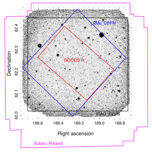
Figure 1: Observation areas in the extended-GOODS-N field. The background image is the CFHT/WIRCam $H$-band image observed in this work. The areas from inside to outside are GOODS-N (red solid line), 2Ms-CDFN (blue solid line), IRAC/SEDS (black solid line), and the Subaru $R$-band image (pink solid line) from Capak et al. (2004).

Table 1: Observation information

Filter	Semester	Integration time	5$\sigma$-limit mag (2″ diameter)	Ref.
$J$	2006A, 2007A, 2009A, 2010A	47 hrs	24.7	Lin et al. (2012) & This work
$H$	2011A, 2012A, 2014A, 2015A	24 hrs	24.2	This work
$K_{s}$	2006A, 2007A, 2008A, 2009A, 2010A	52 hrs	24.4	Wang et al. (2010)

The observation setups in $J$ and $H$ were similar to those used in $K_{s}$ (Wang et al., 2010). Within each observing block (OB), small dithering patterns on the order of tens of arcseconds were used to cover both vertical and horizontal gaps between chips. In each dither position, two to four subframes were taken with a typical exposure time of 60 seconds for $J$ and 15 seconds for $H$. In addition, we offset the centers of dithering by a few arcminutes after each OB to reduce any systematics associated with different chips. The typical seeing for the $J$, $H$, and $K_{s}$ images was between 0$\farcs$7 and 0$\farcs$85 (FWHM). The total integration times in $J$, $H$, and $K_{s}$ are 47, 24, and 52 hours, respectively.

The data were pre-processed using the SIMPLE Imaging and Mosaicking PipeLinE (Wang, 2010). The procedure included flat-fielding, distortion correction, sky subtraction, cross-talk removal, and photometry calibration against the Two Micron All Sky Survey (2MASS; Skrutskie et al., 2006) point-source catalog, as described in detail by Wang et al. (2010) and Lin et al. (2012). The pre-processed frames were further astrometrically calibrated against the Sloan Digital Sky Survey (SDSS) Data Release 6 (DR6) catalog and internal photometry calibrated using the AstrOmatic software Scamp (Bertin, 2006). Finally, all the reduced frames were median stacked using Swarp (Bertin et al., 2002). For the final NIR images, the $5\sigma$ limiting magnitudes (2″ diameter aperture) reach $J=24.7$, $H=24.2$, and $Ks=24.4$.

Figure 2: CFHT/WIRCam $J$, $H$, $K_{s}$ filter transmission curves. The plotted transmissions include the reflectivity of the primary mirror, transmission of the WIRCam optics, atmospheric transmission, and detector efficiency. The three curves are each normalized to a peak value of 1.0.

2.2 Compilation of UV/visible/IR data

Taking the advantage of our deep homogeneous NIR images in the wide field, we assembled publicly released data covering wavelengths from ultraviolet (UV) to mid-infrared (MIR) to compute photometric redshifts (photo-$z$s). The data we collected are as follows:

• UV: The far-UV (FUV) and the near-UV (NUV) data were obtained from the Galaxy Evolution Explorer (GALEX). We matched our NIR-detections (i.e., $z$, $J$, $H$, or $K_{{s}}$-detected sources, see Section 3.1) with the GALEX General Release 6/7 (GR6/7). Although the GALEX image has a point-spread function (PSF) of $\sim$5″, we adopted a search radius of 1″ to decrease the number of sources with contaminated photometry caused by blending. The UV data are used only for the X-ray source counterparts (Section 4.2) and therefore will not affect sources that are not X-ray counterparts.

• Visible: Capak et al. (2004) provided $U$, $B$, $V$, $R$, $I$, $z$ images from the Suprime-Cam on the Subaru telescope with $5\sigma$ limiting magnitudes ranging from 25 to 27 mag. Additionally, we added $y$-band data taken from the Subaru/Suprime-Cam instrument (Ouchi et al., 2009).

• MIR: We used the IRAC 3.6 and 4.5 µm data from SEDS (Ashby et al., 2013). IRAC 5.8 and 8.0 µm data are much shallower than the other two bands, and few objects were detected at these wavelengths. For the SED-fitting process, we used only $\lambda\leq 5$ µm, as suggested in the LePhare manual (page 26), because the stellar light is dominant at these wavelengths.

Table 2 provides detailed information on the photometric data used to calculate the photometric redshifts. In all, 14 bands were used for X-ray counterparts and 12 bands for all other sources.

Table 2: Photometric data

Filter	$\lambda_{\mathrm{eff}}$	FWHM	$5\sigma$ Depth (2″ aperture)	Instrument/Telescope	Reference
	(Å)	(Å)	(AB mag)
FUV	1539	228	25.0	GALEX	General Release 6/7
NUV	2316	796	25.0	GALEX	General Release 6/7
$U$	3584	616	27.03	KPNO Mayall 4 m/MOSAIC	Capak et al. (2004)
$B$	4374	1083	27.01	Subaru/Suprime-Cam	Capak et al. (2004)
$V$	5448	994	26.40	Subaru/Suprime-Cam	Capak et al. (2004)
$R$	6509	1176	26.96	Subaru/Suprime-Cam	Capak et al. (2004)
$I$	7973	1405	25.85	Subaru/Suprime-Cam	Capak et al. (2004)
$z$	9195	1403	25.54	Subaru/Suprime-Cam	Capak et al. (2004)
$y$	9856	585	25.66	Subaru/Suprime-Cam	Ouchi et al. (2009)
$J$	12525	1568	24.7	CFHT/WIRCam	This work
$H$	16335	2875	24.21	CFHT/WIRCam	This work
$K_{s}$	21580	3270	24.41	CFHT/WIRCam	Wang et al. (2010)
3.6 µm	35634	7444	25.0	Spitzer/IRAC	Ashby et al. (2013)
4.5 µm	45110	10119	25.0	Spitzer/IRAC	Ashby et al. (2013)

2.3 X-ray data

X-ray observation is an efficient method to detect active galactic nuclei (AGN). Studies based on the 4 Ms Chandra Deep Field-South (4Ms-CDFS; Xue et al., 2011) and 2 Ms Chandra Deep Field-North Survey (2Ms-CDFN; Alexander et al., 2003; Xue et al., 2016) show that more than 80% of X-ray sources are AGNs. As described by Salvato et al. (2009, 2011), these powerful objects have more complex SEDs than normal galaxies and therefore require special treatment for photo-$z$ estimation. Xue et al. (2016) provided an updated 2Ms-CDFN X-ray catalog, which contains 683 X-ray sources including 196 additional X-ray sources compared to the former catalog from Alexander et al. (2003). We used this X-ray catalog to match with our catalog and identify object to treat as AGNs in the photo-$z$ estimates.

2.4 Spectroscopic data

Spectroscopic redshifts (spec-$z$s) were collected from a number of works, mainly those of Barger et al. (2008), Cowie et al. (2004), Wang et al. (2010), Cooper et al. (2011), and Xue et al. (2016). We matched our NIR detections (see Section 3.1) with spectroscopic data within a maximum separation of 1″. In total, about 3600 sources ($\sim$4%) have spec-$z$ information, and most of them are in the central GOODS-N region. For more reliable estimates of the photo-$z$ quality, we used only 3459 good-quality spec-$z$s as indicated by the quality flag claimed in the literature.

3 Photometry

Table 3: SExtractor parameters

Parameter	Value
DETECT_MINAREA	2
DETECT_THRESH	1.2
ANALYSIS_THRESH	1.2
FILTER	Y
FILTER_NAME	gauss_1.5_3x3.conv
DEBLEND_NTHRESH	64
DEBLEND_MINCONT	0.00001
CLEAN	Y
CLEAN_PARAM	0.1
SEEING_FWHM	0.8
BACK_SIZE	24
BACK_FILTERSIZE	3
BACK_TYPE	AUTO
BACKPHOTO_TYPE	LOCAL
BACKPHOTO_THICK	40
WEIGHT_TYPE	MAP_WEIGHT

3.1 Astrometry and source detection

Figure 3: Astrometric offsets of 12645 sources in common between our $zJHK_{{s}}$ catalog and GOODS-N ACS catalog. Upper left panel shows offsets for individual sources. Right and bottom panels show histograms of offsets in declination and right ascension, respectively.

To combine photometric data from different surveys, we have to make sure that all images are referred to the same astrometric reference frame. Comparing the coordinates in Capak’s visible images with our NIR images, the median values of systematic offsets are $\sim$0$\farcs$3–0$\farcs$4 without any correction. To obtain consistent astrometry, we aligned all the visible images (i.e., $U$, $B$, $V$, $R$, $I$, $z$, and $y$) with the WIRCam $K_{{s}}$-band mosaic. After this calibration, the median values of the systematic offsets between visible and NIR images range from 0$\farcs$13 to 0$\farcs$16. This small offset allows us to do the source detection and flux extraction for all the images on the same astrometric reference frame.

Photometry was extracted based on a detection image created by stacking the non-homogenized NIR (i.e., $J$, $H$, and $K_{{s}}$) and $z$-band images. These wavelengths are sensitive to UV-luminous sources at high redshift (Laigle et al., 2016). The stacked image was created with the CHI2 mode of swarp (Bertin et al., 2002). In this mode, the output image is the square root of the reduced $\chi^{2}$ of pixel values in input images at a given position. This so-called $\chi^{2}$ image was used as the detection image in the dual-image mode of SExtractor to define photometric apertures for each single-band image. In total, 93598 sources were detected.

For photometry extraction, we used astrometry aligned to the WIRCam $K_{{s}}$-band image. However, in the final released catalog, we provide absolute astrometry aligned with the ACS catalog from Giavalisco (2012). Figure 3 compares our $zJHK_{{s}}$ detections with the ACS catalog to show the astrometric offsets. The median values of positional offset in right ascension (R.A.) and declination (Decl.) are 0$\farcs$085 and 0$\farcs$004, respectively.

3.2 PSF homogenization

Our 10 ground-based images ($U$, $B$, $V$, $R$, $I$, $z$, $y$, $J$, $H$, $K_{s}$) have FWHMs of the PSF ranging from 0$\farcs$8 to 1$\farcs$3. This will give inaccurate flux densities if the same fixed-size aperture is adopted for all the bands because the ratio of aperture flux density to total flux density will depend on PSF size. In order to obtain accurate total flux densities and colors, which can be used to fit the SEDs and compute photo-$z$s, we need to take the varying PSFs into account. We adopted the approach of Capak et al. (2007), degrading the better-seeing images to the largest PSF (that of the $U$-band image) of 1$\farcs$3 using a Gaussian kernel appropriate to each image. To be specific, we used the PSF characterization (calculating FWHM on images) and equalization (smoothing with a Gaussian kernel) tools in the Subaru SuprimeCAM reduction package (sdfred) in iraf.

Because the PSF sizes of GALEX and IRAC are very large, to avoid blending, we didn’t include UV and IRAC data in the PSF homogenization. Instead we obtained the UV total flux densities directly through the GALEX online query system “CasJobs”. The IRAC total flux densities were extracted with the improved IRACLEAN (Hsieh et al., 2012; Laigle et al., 2016), which is designed especially for IRAC.

3.3 Visible/NIR photometry

3.3.1 Absolute photometry of NIR images

The absolute photometry of our WIRCam $J$, $H$, $K_{s}$ images was calibrated with 2MASS (i.e., The Two Micron All Sky Survey) point sources in the observed field. Figure 4 shows the magnitude differences between the 2MASS and the calibrated WIRCam magnitudes. The scatter becomes larger at mag $<14.5$ and $>16.5$. The magnitude differences are mostly constant between 14.5 mag (the brightest WIRCam sources) and 16.5 mag (where 2MASS $S/N$ deteriorates). We therefore chose the median value in the range $14.5<\rm{mag}<16.5$ to set the calibration for each WIRCam NIR image. In the $J$-band, there are some sources with large scatter at $J<15.5$. Most of these are saturated stars, and their WIRCam photometry is not reliable. However, these sources do not affect our calibrations.

As mentioned by Wang et al. (2010), the magnitude uncertainties in Figure 4 are dominated by 2MASS. Therefore our NIR flux calibration is limited by the 2MASS systematic uncertainty.

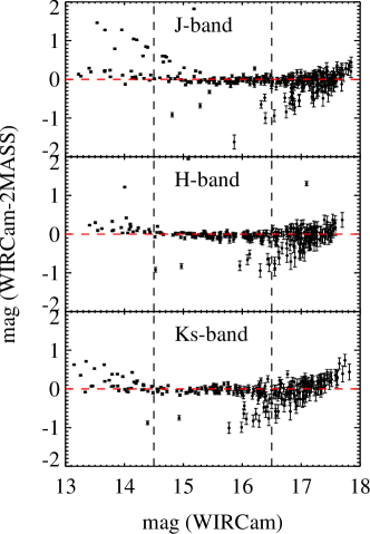
Figure 4: Magnitude differences between 2MASS and the calibrated WIRCam AB magnitude in $J$, $H$, $K_{s}$. The 1$\sigma$ combined uncertainties are plotted as vertical error bars. The horizontal red dashed-lines indicate magnitude differences of zero. The two vertical black dashed-lines indicate magnitude = 14.5 and 16.5.

3.3.2 $U$ to $K_{s}$ flux extraction

As mentioned above, $U$ to $K_{s}$ photometry was performed with SExtractor in dual-image mode. We used the $zJHK_{{s}}$ $\chi^{2}$ image as the detection image and measured aperture photometry on each PSF-homogenized image. Fixed-aperture flux densities (i.e., FLUX_APER) have higher signal-to-noise ratio than the automatic-aperture flux densities (i.e., FLUX_AUTO) (Kron, 1980). Therefore, fixed-aperture photometry gives “cleaner” colors for SED fitting and more accurate photo-$z$s. Tests showed that 2″ FLUX_APER gave better photo-$z$ quality (i.e., better accuracy and fewer outliers) than either FLUX_AUTO or 3″ FLUX_APER. We therefore used 2″-aperture photometry for photo-$z$ computation. However, both 2″ FLUX_APER and FLUX_AUTO are included in the released catalog.

The SExtractor parameters we used are mainly adopted from Wang et al. (2010) and Hsieh et al. (2012), who observed with the same instrument (i.e., CFHT/WIRCam) as we did. The parameter CLEAN_PARAM in particular is critical for source detection. We examined values of CLEAN_PARAM from 0.1 to 1.0 and found that the number of detections increased from ${\sim}90000$ to ${\sim}130000$. Setting $\texttt{CLEAN\_PARAM}=0.1$ avoids a large number of false detections as demonstrated by Yang et al. (2014). We also visually inspected random sources on the images and confirmed that false detections are greatly reduced with a lower value of CLEAN_PARAM. Table 3 lists the main SExtractor parameters used to obtain the photometry.

Because GALEX and IRAC photometry is provided as total flux density, to combine them with visible and NIR photometry, we need to convert visible and NIR aperture flux densities to total flux densities for each band using the equation:

$${f_{tot}=f_{\rm aper}\times{\rm median}\left(\frac{f_{\rm auto}}{f_{\rm aper}}\right)\times 1.06}\quad.$$ (1)

First we converted the fixed-aperture flux densities ($f_{\rm aper}$) to automatic-aperture flux densities ($f_{\rm auto}$) by multiplying the median ratio between FLUX_AUTO and FLUX_APER. FLUX_APER misses about 5 to 10% of the flux density, and therefore we multiplied by the factor 1.06, the same value adopted by Yang et al. (2014).

3.3.3 Photometric uncertainties

It is essential to have accurate photometric uncertainties for measuring accurate photo-$z$s. However the uncertainties generated by SExtractor are usually underestimated because of correlated noise among pixels. Therefore, following Bielby et al. (2012), we computed the rms of flux densities measured in random blank sky positions with 2″ apertures. Blank sky positions were identified from the segmentation map generated by SExtractor. Then we calculated the ratio between the derived rms in the field and the mean value of the SExtractor uncertainties of all objects. These ratios—1.5, 1.72, and 1.78 in $J$, $H$, and $K_{s}$ bands, respectively—should be the correction factors. To be conservative, we applied a correction factor of 2 to the SExtractor uncertainties in all the bands before computing the photo-$z$s. This correction is not included in the photometric errors in the released catalog, which gives the errors output by SExtractor.

3.4 IRAC photometry

IRAC images have PSFs with FWHM around 1$\farcs$8 (IRAC Instrument Handbook), larger than the visible and NIR bands. Therefore they require different procedures for deblending objects and determining the flux densities accurately. Several methods have been developed for performing IRAC flux density measurements. In this work, we used the algorithm IRACLEAN (Hsieh et al., 2012). The method was further improved (Laigle et al., 2016) to obtain more accurate flux densities for blended objects with large flux differences and separations less than one FWHM. Unlike other methods that first deconvolve high-resolution images with high-resolution PSFs and then convolve with the low-resolution PSFs, the IRACLEAN approach merely deconvolves the IRAC low-resolution images with the IRAC PSFs and adopts source positions and surface brightnesses as priors to derive the IRAC flux densities. Without requiring identical morphologies for each object (as other methods do), this method minimizes the effect of morphological k-correction (see Hsieh et al. 2012 and Laigle et al. 2016 for details).

In the IRACLEAN procedure, we used the high-resolution WIRCam $zJHK_{{s}}$ $\chi^{2}$ image as a prior for the low-resolution IRAC photometry. The IRAC flux densities were registered to the associated detections in the stacked-$zJHK_{{s}}$ segmentation map generated by SExtractor. The uncertainty was estimated from fluctuations in the local area for each object in the residual map, taking the non-independence of mosaic pixels into account.

3.5 Completeness

We used simulations, performed separately for each WIRCam filter, to characterize the completeness functions of the WIRCam observations. Artificial stars of different magnitudes were generated and added to the reduced WIRCam images. Then we applied the same source extraction technique to detect and extract photometry. These artificial stars were recovered or missed depending on their flux, local noise, crowding, etc. Thus the completeness of photometry in each filter was evaluated as a function of magnitude based on the fraction of recovered artificial stars input in the reduced image (Figure 5). The limiting magnitudes corresponding to 95% completeness are 24.4, 23.7, and 23.7 in the $J$, $H$ and $K_{s}$ bands, respectively.

In fact, most of our detections are extended sources. To be more realistic, for $J$ and $H$ bands, we compared the number density of our detections with the deeper HST/WFC3 observation from the 3D-HST catalog (Skelton et al., 2014) to deduce the completeness (Figure 6). We assumed that the 3D-HST catalog is complete at magnitudes less than 26 in $J$ and $H$ bands, and our catalog reaches 99% completeness in $J$ and $H$ bands at 24.5 and 24.2 mag, respectively. Indeed the number densities of our work at some points are higher than the 3D-HST catalog. This could be due to the different filter bandpasses. For $K_{s}$ bands, however, no public image is deep enough for us to do this measurement in this field. Therefore we extrapolated from the $K_{s}$-band number density to estimate 99% completeness at 23.9 mag.

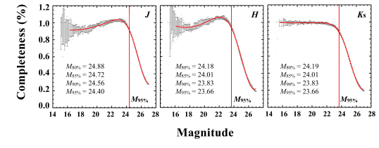
Figure 5: Completeness estimated by simulated stars for the $J$, $H$, and $K_{s}$ band data (fitted with red solid curves from left to right panels). The red vertical lines mark the limiting magnitudes for $95\%$ completeness. Magnitudes for other completeness values (from $80\%$ to $90\%$ ) are given in each panel.

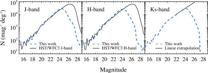
Figure 6: Comparisons of number densities between our work (blue dashed-lines) and the 3D-HST catalog (black solid lines) in $J$ and $H$ bands. In $K_{s}$ band, the black solid line shows the linear curve extrapolated based on the best fit in the magnitude range from 22 to 24 mag.

4 Photometric redshifts

We computed photo-$z$s using the publicly available code LePhare (Arnouts et al., 1999; Ilbert et al., 2006), which is based on $\chi^{2}$ minimization for obtaining the best-fit template. We divided the source catalog into non-X-ray-detected and X-ray-detected subsamples and applied an appropriate template library for each subsample separately. For non-X-ray-detected sources, we fitted with pure galaxy templates, whereas for the X-ray-detected sources, we fitted with AGN-galaxy hybrid templates. In addition, we fitted both subsamples with stellar SED templates to identify stars. In the following photo-$z$ quality analysis, we excluded not only spectroscopically-confirmed (spec-$z$ = 0) stars but also SED-classified stars defined by $\chi_{\rm star}^{2}<\chi_{\rm best}^{2}$. In the whole spectroscopic sample, there are 240 SED-classified stars, and 196 ($\sim$82%) of them are spectroscopically confirmed.

Sources with spec-$z$ (denoted by $z_{s}$) information were used to quantify the photo-$z$ (denoted by $z_{p}$) performance. Three parameters quantify the photo-$z$ quality: $\sigma_{\mathrm{NMAD}}$, $\eta$, and $b_{z}$. We measured the normalized median absolute deviation $\sigma_{\mathrm{NMAD}}\equiv 1.48\times\mathrm{median}(\frac{|\Delta z|}{1+z_{s}}$), where $\Delta z\equiv(z_{p}-z_{s})$. Outliers were not removed before computing $\sigma_{\mathrm{NMAD}}$. We defined outliers by $\frac{|\Delta z|}{1+z_{s}}>0.15$, and $\eta$ indicates the fraction of outliers. $b_{z}$ is defined by $\frac{\Delta z}{1+z_{s}}$ which indicates the difference between photo-$z$ and spec-$z$, and $\overline{b_{z}}$ is the mean value of $b_{z}$ after excluding the outliers. Figure 7 shows the photo-$z$ and spec-$z$ distributions. The majority of sources with spectra have $z_{s}<1.5$.

Figure 7: Spec-$z$ and photo-$z$ distributions in this work.

Table 4: Photo-$z$ quality for non-X-ray and X-ray sources.

	Non-X-ray sources				X-ray sources
	$N$	$\overline{b_{z}}$	$\sigma_{\mathrm{NMAD}}$	$\eta(\%)$	$N$	$\overline{b_{z}}$	$\sigma_{\mathrm{NMAD}}$	$\eta(\%)$
Total	2861	$-0.013$	0.036	7.34	352	$-0.003$	0.040	10.51
$R<23$	0947	$-0.011$	0.025	1.58	229	00.001	0.036	6.99
$R>23$	1914	$-0.014$	0.044	10.19	123	$-0.012$	0.054	17.07
$z<1.0$	1893	$-0.013$	0.034	4.07	224	00.001	0.035	5.36
$z>1.0$	0967	$-0.012$	0.042	13.75	128	$-0.011$	0.054	19.53

4.1 Non-X-ray sources

4.1.1 Galaxy templates

For the non-X-ray-detected sources, we applied the same templates as used by Ilbert et al. (2009) in the Cosmic Evolution Survey (COSMOS) field. The templates are well-verified SED templates for galaxies and have been used in many works (e.g., Salvato et al., 2009; Ilbert et al., 2013; Hsu et al., 2014; Laigle et al., 2016). The library contains 31 templates including 19 galaxies from Polletta et al. (2007) and 12 young, star-forming galaxies from Bruzual & Charlot (2003) models. LePhare adds emission lines to the galaxy templates during the fitting process (see Section 3.2 of Ilbert et al. 2009). These lines ([O II], [O III], H$\beta$, H$\alpha$, and Ly$\alpha$) were estimated from fixed ratios to the UV luminosity as defined by Kennicutt (1998). This helps characterize star-forming galaxies that have strong emission lines in their SEDs.

The extinction laws adopted in the fitting were from Prevot et al. (1984) and Calzetti et al. (2000) plus two additional models with modifications of the 2170Å bump based on the Calzetti et al. extinction laws. We allowed the parameter $E(B-V)$ to range from 0.00 to 0.50 in steps of 0.05 mag. As described by Ilbert et al. (2009), we set a prior of absolute magnitude range to be $-24<M_{B}<-8$ (typical for normal galaxies) during the fitting procedure to reduce the degeneracy.

Systematic differences can occur in each band between our photometry and predicted photometry based on the best-fit template selected during the photo-$z$ computation. Using the code LePhare, we derived zero-point offsets with the training sample (randomly selected $\sim$800 non-X-ray sources) to correct the systematic differences for all the sources. The same corrections were applied to X-ray objects.

4.1.2 Photo-$z$ results

The photo-$z$ result using 12 bands (i.e., $U$, $B$, $V$, $R$, $I$, $z$, $y$, $J$, $H$, $K_{s}$, 3.6 and 4.5 µm) is shown in Figure 9. We achieved an overall accuracy $\sigma_{\mathrm{NMAD}}=0.036$ with an outlier fraction $\eta=7.3\%$ from the comparison between photo-$z$ and spec-$z$. For the bright ($R<23$) sources, we obtained $\sigma_{\mathrm{NMAD}}=0.025$ and $\eta=1.58\%$. For low-redshift ($z<1.0$) sources, we obtained $\sigma_{\mathrm{NMAD}}=0.034$ and $\eta=4.0\%$ (Table 4).

There are several possible reasons for photo-$z$ outliers. The first is uncertain photometry, including faint or blended objects. (See two examples in Figure 8.) Second, outliers could be due to the absence of representative templates in the library. For instance, Onodera et al. (2012) found that photo-$z$s in the Ilbert et al. (2009) sample are often underestimated for quiescent galaxies at $1.5<z<2$. Third, misinterpreting a spectral break as Lyman break or Balmer break could lead to a catastrophic failure of photo-$z$ (Dahlen et al., 2010). Fourth, the broad-band data points may miss or mis-fit emission lines in the SEDs. In this case, as demonstrated by Ilbert et al. (2009) and Salvato et al. (2009), medium- or narrow-band data can help to pinpoint the emission line features and significantly improve the photo-$z$ quality. Due to the lack of medium- or narrow-band data in this work, it is not surprising that we are not able to achieve the same photo-$z$ qualities as presented in other deep fields such as COSMOS and CDFS. The upcoming Survey for High-$z$ Absorption Red and Dead Sources (SHARDS; Pérez-González & Cava, 2013) will help to improve the photo-$z$ quality in GOODS-N region.

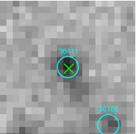
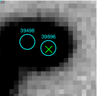
Figure 8: Two examples of photo-$z$ outliers in $R$-band negative images 6″$\times$6″ in size. Green crosses mark the spec-$z$ positions, and cyan open circles 1″ in diameter indicate the $zJHK_{{s}}$ detections. The left source is faint with most of of its visible magnitude $>$25. The right source is blended, and its photometry is contaminated.

Figure 9: Upper panel: spec-$z$ vs. photo-$z$ for non-X-ray sources (black dots) in this work. The solid line indicates $z_{p}=z_{s}$; the two dotted lines embrace the $z_{p}=z_{s}\pm 0.15(1+z_{s})$. Lower panel shows $\Delta z\equiv(z_{p}-z_{s})$.

4.2 X-ray sources

Because the majority of X-ray detections are associated with AGNs, we cannot use pure galaxy templates to fit their SEDs. A separate set of AGN-galaxy hybrid templates is required.

4.2.1 Cross-matching

The first step in computing photo-$z$s for X-ray sources was to cross-match our $zJHK_{{s}}$ detections to the 2Ms-CDFN X-ray catalog (Xue et al., 2016). The X-ray source positions used $K_{s}$-band images from Wang et al. (2010) as the reference frame, which is the same as ours. The median offset between the X-ray positions and our $zJHK_{{s}}$ positions is 0$\farcs$2. This value is smaller than the median value of X-ray positional uncertainty (0$\farcs$6). Therefore, we adopted a simple search radius of 1″ to match our $zJHK_{{s}}$ detections with X-ray sources. 602 X-ray sources have $zJHK_{{s}}$ detections within this search radius. Xue et al. (2016) used likelihood-ratio matching to identify the visible/near-infrared/mid-infrared/radio (ONIR) counterparts. We compared their positions to those of our $zJHK_{{s}}$ counterparts. When more than one $zJHK_{{s}}$ detection was found within the search radius, we chose the one closest to the ONIR counterpart. $zJHK_{{s}}$ counterparts within 1″ radius are labeled “xflag=1” in the catalog.

For the remaining 81 X-ray sources lacking counterparts within the 1″ search radius, we checked their multi-band cutouts visually. 56 of them have $zJHK_{{s}}$ detections nearby that are consistent with the ONIR counterparts from Xue et al. (2016), as shown in Figure 10. In our released catalog, we treated these 56 sources as the $zJHK_{{s}}$ counterparts of the X-ray sources and provided photo-$z$ measurement of them. The photo-$z$s of these 56 sources should be used with caution because of the large separation as shown in Figure 10. These sources are labeled “xflag=2” in the catalog.

In total, 25 out of 683 X-ray sources have no $zJHK_{{s}}$ counterparts. With visual inspection, we group these 25 sources into three cases:

• Case 1: 8 sources that are only detected by IRAC (Figure 11a);

• Case 2: 13 sources that have no $zJHK_{{s}}$ or IRAC detections around the X-ray detection (Figure 11b);

• Case 3: 4 sources that have highly extended $zJHK_{{s}}$ sources nearby. These sources have a large offset to the X-ray source position and therefore are not likely counterparts (Figure 11c).

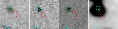
Figure 10: Example of multi-band cutouts for one X-ray source with $zJHK_{{s}}$ counterpart separated by more than 1″ from the Xue et al. (2016) ONIR counterpart position. From left to right, negative images show $R$, $z$, $H$, and IRAC 3.6 $\mu$m. Images are 8″$\times$8″ on a side. Yellow crosses mark the ONIR counterparts found by Xue et al. (2016), cyan open circles mark the corresponding $zJHK_{{s}}$ detection from this work, and red open circles mark the X-ray positions with radius being the positional uncertainty. In this case, the separation between the X-ray source ([XLB2016 CDFN] 32) and the $zJHK_{{s}}$ detection is about 2″.

In Case 1 above, the IRAC sources can be considered the correct identifications for the X-ray sources. However, because Case 1 has only IRAC photometry, we cannot compute photo-$z$s for these eight sources. In Case 2, 11 of them have either no $zJHK_{{s}}$ or ONIR counterparts around the X-ray detection, whereas the remaining two X-ray sources have ONIR counterparts in bluer bands but no $zJHK_{{s}}$ detections. For Case 3, the extended $zJHK_{{s}}$ sources are likely foreground galaxies that hide the true counterpart. We have excluded objects in all three cases above from the subsequent analysis for the X-ray sources.

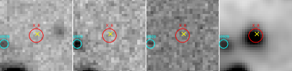
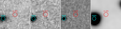
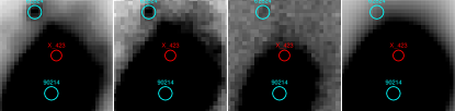
Figure 11: Three examples of multi-band cutouts for X-ray sources without $zJHK_{{s}}$ counterparts. From left to right are $R$, $z$, $H$, and IRAC 3.6 $\mu$m negative images 8″$\times$8″ on a side. Yellow crosses mark the ONIR counterparts (Xue et al., 2016), cyan open circles mark the corresponding $zJHK_{{s}}$ detections from this work, and red open circles mark the X-ray positions with radius being the positional uncertainty. From top to bottom are [XLB2016 CDFN] 8, 275, and 423 respectively.

4.2.2 AGN-galaxy hybrid training

After cross-matching, we computed photo-$z$s for the X-ray sources in the CDFN. We applied the AGN-galaxy hybrid templates built by Hsu et al. (2014), which were trained on the X-ray sources detected in the 4Ms-CDFS survey. Each AGN-galaxy hybrid is composed of a galaxy template and an AGN template with ratios varying from 1:9 to 9:1. The galaxy templates are from Bender et al. (2001), and the AGN templates are from Polletta et al. (2007). The best set of hybrid templates were tuned using randomly-selected $25\%$ of the X-ray sources from the 4Ms-CDFS catalog. The AGN-galaxy hybrid libraries used here contain 48 and 30 best-fit templates for optically extended sources and point-like sources, respectively. Details were given by Hsu et al. (2014).

During the SED fitting process for the X-ray sources, we adopted the same systematic offsets and extinction laws as used for the non-X-ray sources. For an absolute magnitude prior, we used $-24<M_{B}<-8$ for extended X-ray counterparts and $-30<M_{B}<-20$ for point-like X-ray counterparts (Salvato et al., 2009).

4.2.3 Photo-$z$ results

The UV bump from an AGN accretion disk is a significant spectral feature for distinguishing an AGN from a non-active galaxy. Therefore, UV data are particularly important for obtaining accurate photo-$z$s for AGNs, as demonstrated by Hsu et al. (2014). 222 out of 683 X-ray sources are detected in either FUV or NUV. For these sources, we included UV data in addition to the same 12 bands used for the non-X-ray objects when computing photo-$z$s. As shown in Table 4 and Figure 12, we achieved an overall $\sigma_{\mathrm{NMAD}}$ for X-ray counterparts almost as good as that for non-X-ray sources. The outlier fraction was higher, especially for fainter sources and those at $z>1$. To demonstrate the benefit of UV data, we compared photo-$z$ results with and without UV data for 174 X-ray sources that have spec-$z$. Figure 13 shows that $\sigma_{\mathrm{NMAD}}$ is almost unchanged, but the outlier fraction $\eta$ decreases from $9.8\%$ without UV data to $6.3\%$ when UV data are added.

The causes of the catastrophic failures of photo-$z$s for the X-ray sources are more complicated than for the non-X-ray sources. In addition to the reasons discussed in Section 4.1.2, the outliers could be also due to variability (Salvato et al., 2009) and to the uncertain contributions from AGNs.

In our released catalog, for both X-ray and non-X-ray sources, $z_{p}$ is defined by the peak value of the redshift probability distribution function $p(z)$. Figure 14 shows three examples of our results. In some cases (e.g., the object [HLD2018]=47637 in Figure 14), there are two or more peaks in the probability distribution function. In such situations, we defined photo-$z$ as the highest peak of $p(z)$.

Figure 12: Spec-$z$ vs. photo-$z$ for all the X-ray sources (black dots) with spec-$z$ in this work. The solid line indicates $z_{p}=z_{s}$; the two dotted lines embrace the $z_{p}=z_{s}\pm 0.15(1+z_{s})$. Lower panel shows $\Delta z\equiv(z_{p}-z_{s})$.

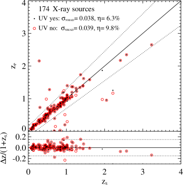
Figure 13: Spec-$z$ vs. photo-$z$ for 174 X-ray sources that have either FUV or NUV data. The black dots indicate the photo-$z$ computed with UV data, and the red open circles indicate the photo-$z$ computed without UV data.

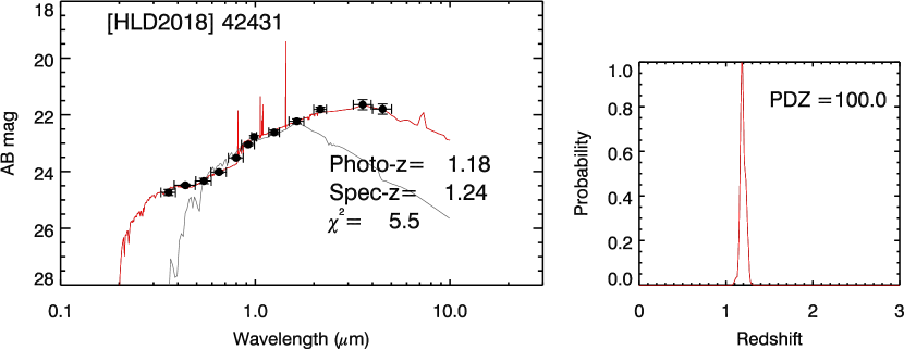
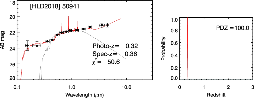
Figure 14: Examples of SED fitting. Left panels show the observed data points (black filled circles) with the best-fit templates (red solid line) and stellar templates (grey solid line). Right panels show the corresponding redshift probability distribution function $p(z)$. The sources from top to bottom are [HLD2018] 42431, 50941, and 47637, respectively. The first one is a non-X-ray source fitted with a galaxy template. The two below are X-ray sources fitted with AGN–galaxy hybrid templates. The PDZ is the normalized integration of $p(z)$ between $z_{p}\pm 0.1(1+z_{p})$. Higher values of PDZ indicates higher probability of the given $z_{p}$.

4.3 Comparison with previous work

Yang et al. (2014) used the code EAzY (Brammer et al., 2008) to estimate photo-$z$s for sources in the field. The main differences between our work and theirs are: (1) the templates used for SED fitting. Yang et al. (2014) used only 8 galaxy templates for non-X-ray sources and added 3 QSO templates for X-ray sources. We used 31 galaxy templates for non-X-ray sources and 78 galaxy or galaxy–AGN hybrid templates for X-ray sources. (2) the integration time of the NIR images. The NIR data we used are $0.5-1.0$ mag deeper. (3) the X-ray catalog. Yang et al. (2014) used the Alexander et al. (2003) X-ray catalog, whereas we used the one from Xue et al. (2016). (4) UV data. We added UV data to compute photo-$z$s for the X-ray sources. For 2842 non-X-ray sources with spec-$z$s in common between our work and Yang et al. (2014), the two studies achieved comparable quality ($\sigma_{\mathrm{NMAD}}=0.036$, $\eta=7.1\%$). At $z<1$, both works have similar error distributions as shown in Figure 15. At $z>1$, our work is more peaked near $\frac{\Delta z}{1+z_{s}}=0$ and has smaller scatter ($\sigma_{\mathrm{NMAD}}=0.042$), whereas Yang et al. (2014) tended to underestimate photo-$z$s and had slightly larger scatter ($\sigma_{\mathrm{NMAD}}=0.048$).

For the X-ray sources, Xue et al. (2016) adopted two main photo-$z$ catalogs (Yang et al., 2014; Skelton et al., 2014). Table 5 lists the comparisons for the 269 sources in common among all three works. Our photo-$z$ accuracy is similar to that of Yang et al. (2014). The accuracy of the 3D-HST catalog (Skelton et al., 2014) is better than the other two studies for both X-ray and non-X-ray sources because Skelton et al. (2014) used the extremely deep visible and NIR data from HST. However, Skelton et al. (2014) fitted the X-ray sources with normal galaxy templates, and that gave a larger outlier fraction ($11.9\%$) compared to ours ($8.6\%$). Figure 16 compares our $\frac{\Delta z}{1+z_{s}}$ distribution with the two other studies. Although Yang et al. achieved slightly lower outlier fraction than we did, their $\frac{\Delta z}{1+z_{s}}$ distribution for X-ray sources has a negative offset (see the upper panel in Figure 16), which was also mentioned by Xue et al. (2016). This is probably caused by systematic errors. The offsets of $\frac{\Delta z}{1+z_{s}}$ are quantified by $\overline{b_{z}}$ in Table 5.

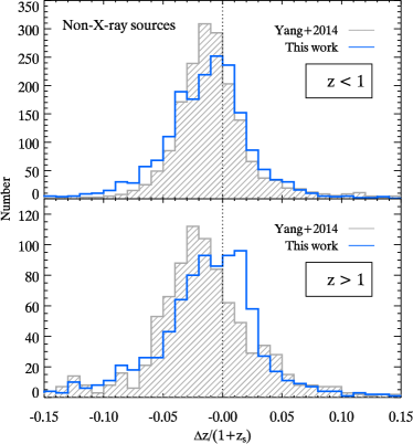
Figure 15: Comparison of the $\frac{\Delta z}{1+z_{s}}$ distribution for the non-X-ray sources with the previous work of Yang et al. 2014 at $z<1$ (upper panel) and $z>1$ (lower panel).

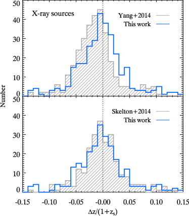
Figure 16: Comparison of the $\frac{\Delta z}{1+z_{s}}$ distribution for the X-ray sources with the previous studies of Yang et al. 2014 (upper panel) and Skelton et al. 2014 (lower panel).

5 Column description for the released catalogs

We release photometry and photo-$z$ catalog as shown in Table 6. We also release the NIR images online. All data are available through the portal: http://idv.sinica.edu.tw/lthsu. Below are the descriptions for the table columns.

• Column 1 ([HLD2018]) gives the sequence number of $zJHK_{{s}}$ detections.

• Column 2 (R.A.) gives the J2000 right ascension of $zJHK_{{s}}$ detections.

• Column 3 (Decl.) gives the J2000 declination of $zJHK_{{s}}$ detections.

• Column 4 ($z_{s}$) gives the spectroscopic redshift. The value $-99$ indicates that no $z_{s}$ is available.

• Column 5 ($Q_{{s}}$) gives the spectroscopic redshift quality. The value 1 indicates that the $z_{s}$ is good, and the value 2 indicates that the $z_{s}$ is uncertain. The value $-99$ indicates that no value is available.

• Column 6 ($z_{p}$) gives the best-fit photo-$z$, which is the highest peak in the associated redshift distribution function $p(z)$. (See the examples in Figure 14.) The value $-99$ indicates that no $z_{p}$ is available.

• Column 7 ($1\sigma^{\rm{low}}$): lower 1$\sigma$ value of $z_{p}$ estimated from the equation $\chi^{2}(z)=\chi^{2}_{\rm{min}}+1$, where $\chi^{2}_{\rm{min}}$ is the minimum of $\chi^{2}$ (Ilbert et al., 2009).

• Column 8 ($1\sigma^{\rm{up}}$): upper 1$\sigma$ value of $z_{p}$.

• Column 9 ($\chi^{2}_{\rm{best}}$): $\chi^{2}$ for the best galaxy fit for non-X-ray sources or AGN–galaxy fit for X-ray sources.

• Column 10 ($\chi^{2}_{\rm{star}}$): $\chi^{2}$ for the best stellar fit.

• Column 11 (PDZ): a measure of the probability of $z_{p}$: the integral of the normalized probability distribution function $p(z)$ between $z_{p}\pm 0.1(1+z_{p})$. A higher value of PDZ indicates higher probability of the given $z_{p}$.

• Column 12 (xflag): marks whether a $zJHK_{{s}}$ source is considered as the counterpart of a given X-ray source. xflag = 1 indicates a $zJHK_{{s}}$ source separated by less than 1″ from an X-ray source. xflag = 2 indicates a $zJHK_{{s}}$ separated from an X-ray source ${>}$1″. $\mathrm{xflag}=-99$ indicates $zJHK_{{s}}$ source not considered a counterpart of any X-ray source. Section 4.2.1 describes the counterpart identification process.

• Column 13 ([XLB2016 CDFN]) is the sequence number for the X-ray source given from the 2Ms-CDFN X-ray catalog (Xue et al., 2016). The value $-99$ indicates that the source has no X-ray counterpart.

• Column 14 (XRA) is the J2000 right ascension of the X-ray source in the 2Ms-CDFN X-ray catalog. The value $-99$ indicates that the source has no X-ray counterpart.

• Column 15 (XDEC) is the J2000 declination of the X-ray source in the 2Ms-CDFN X-ray catalog. The value $-99$ indicates that the source has no X-ray counterpart.

• Columns 16–19 give the total flux densities and uncertainties for FUV and NUV queried from GALEX GR6/7.

• Columns 20–39 give the 2″ diameter aperture flux densities and associated uncertainties from SExtractor output parameters FLUX_APER and FLUXERR_APER for $U$, $B$, $V$, $R$, $I$, $z$, $y$, $J$, $H$, $K_{{s}}$, respectively. Each flux density is immediately followed by its uncertainty. Unit of flux density is $\mu$Jy .

• Columns 40–59 give the flux densities and associated uncertainties from SExtractor output parameters FLUX_AUTO and FLUXERR_AUTO for $U$, $B$, $V$, $R$, $I$, $z$, $y$, $J$, $H$, $K_{{s}}$, respectively.

• Columns 60–63 give the total flux densities and uncertainties for IRAC 3.6 and 4.5 $\mu\rm{m}$ based on IRACLEAN.

Table 5: Comparison of our X-ray-source photo-$z$ quality with recent work

		This work			Yang et al. (2014)			Skelton et al. (2014)
	$N$	$\overline{b_{z}}$	$\sigma_{\mathrm{NMAD}}$	$\eta(\%)$	$\overline{b_{z}}$	$\sigma_{\mathrm{NMAD}}$	$\eta(\%)$	$\overline{b_{z}}$	$\sigma_{\mathrm{NMAD}}$	$\eta(\%)$
Total	269	-0.003	0.039	8.55	-0.014	0.040	7.43	0.001	0.032	11.90
$R<23$	170	0.000	0.036	4.12	-0.016	0.035	2.94	0.002	0.030	7.06
$R>23$	99	-0.011	0.055	16.16	-0.009	0.053	15.15	-0.002	0.042	20.20
$z<1.0$	169	-0.001	0.037	3.55	-0.015	0.037	4.73	0.005	0.030	5.33
$z>1.0$	100	-0.007	0.053	17.00	-0.012	0.048	12.00	-0.008	0.043	23.00

Table 6: Released photometric catalog

[HLD2018]	R.A.	Decl.	$z_{s}$	$Q_{\rm{spec}}$	$z_{p}$	$1\sigma^{\rm{low}}$	$1\sigma^{\rm{up}}$	$\chi^{2}_{\rm{best}}$	$\chi^{2}_{\rm{star}}$	PDZ	xflag
(1)	(2)	(3)	(4)	(5)	(6)	(7)	(8)	(9)	(10)	(11)	(12)
18637	189.264864	62.0859387	$-99$	$-99$	0.9024	0.8956	0.9104	44.6636	429.492	100	1
18709	189.1442586	62.0872443	0.6346	1	0.6243	0.616	0.6328	16.4447	731.437	100	$-99$
18837	189.3097146	62.0846307	$-99$	$-99$	0.423	0.4187	0.4255	75.3598	3006.53	100	1
18864	189.2370479	62.0831875	$-99$	$-99$	0.8087	0.794	0.8219	91.5799	903.539	100	1
19099	189.1462737	62.0888751	0.9876	1	0.9252	0.9181	1.0144	36.7712	4045.29	100	$-99$
19416	189.1381716	62.0901795	$-99$	$-99$	0.3834	0.38	0.3801	2650.6	172.872	100	$-99$

6 Summary

Homogeneous NIR images ($J$, $H$, and $K_{s}$) taken by the instrument CFHT/WIRCam in the extended GOODS-N achieve 5$\sigma$ limiting AB magnitudes in 2″ diameter apertures of 24.7, 24.2, and 24.4 mag in the $J$, $H$, and $K_{s}$ bands, respectively. The images are released along with the multi-band photometry and photometric redshift catalog, which contains $93598$ $zJHK_{{s}}$ detections.

1. For the non-X-ray sources, we obtained accuracy $\sigma_{\mathrm{NMAD}}=0.025$ and an outlier fraction $\eta=1.58\%$ for the $R<23$ sources. For the overall sample, we reached $\sigma_{\mathrm{NMAD}}=0.036$ with $\eta=7.3\%$.

2. For the X-ray sources, identified with the updated X-ray catalog from Xue et al. (2016), $\sigma_{\mathrm{NMAD}}=0.040$ with $\eta=10.5\%$. This outlier fraction is smaller than that of previous work from the 3D-HST catalog.

3. The use of UV data for the X-ray sample slightly improves the photo-$z$ accuracy and reduces $\eta$ from $9.8\%$ to $6.3\%$.

These data provide a large sample of objects to study galaxy formation and evolution and the coevolution between AGNs and their host galaxies. Future updates of the catalog will be on the website: http://idv.sinica.edu.tw/lthsu. Upcoming medium- or narrow-band data, e.g., SHARDS, will improve photo-$z$ quality, especially for AGNs and star-forming galaxies whose emission lines are usually strong.

References

- Alexander et al. (2003) Alexander, D. M., Bauer, F. E., Brandt, W. N., et al. 2003, AJ, 126, 539, doi: 10.1086/376473
- Arnouts et al. (1999) Arnouts, S., Cristiani, S., Moscardini, L., et al. 1999, MNRAS, 310, 540, doi: 10.1046/j.1365-8711.1999.02978.x
- Ashby et al. (2013) Ashby, M. L. N., Willner, S. P., Fazio, G. G., et al. 2013, ApJ, 769, 80, doi: 10.1088/0004-637X/769/1/80
- Ashby et al. (2015) —. 2015, ApJS, 218, 33, doi: 10.1088/0067-0049/218/2/33
- Barger et al. (2008) Barger, A. J., Cowie, L. L., & Wang, W.-H. 2008, ApJ, 689, 687, doi: 10.1086/592735
- Bender et al. (2001) Bender, R., Appenzeller, I., Böhm, A., et al. 2001, in Deep Fields, ed. S. Cristiani, A. Renzini, & R. E. Williams, 96
- Bertin (2006) Bertin, E. 2006, in Astronomical Society of the Pacific Conference Series, Vol. 351, Astronomical Data Analysis Software and Systems XV, ed. C. Gabriel, C. Arviset, D. Ponz, & S. Enrique, 112
- Bertin & Arnouts (1996) Bertin, E., & Arnouts, S. 1996, A&AS, 117, 393, doi: 10.1051/aas:1996164
- Bertin et al. (2002) Bertin, E., Mellier, Y., Radovich, M., et al. 2002, in Astronomical Society of the Pacific Conference Series, Vol. 281, Astronomical Data Analysis Software and Systems XI, ed. D. A. Bohlender, D. Durand, & T. H. Handley, 228
- Bielby et al. (2012) Bielby, R., Hudelot, P., McCracken, H. J., et al. 2012, A&A, 545, A23, doi: 10.1051/0004-6361/201118547
- Bouwens et al. (2010) Bouwens, R. J., Illingworth, G. D., González, V., et al. 2010, ApJ, 725, 1587, doi: 10.1088/0004-637X/725/2/1587
- Bouwens et al. (2015) Bouwens, R. J., Illingworth, G. D., Oesch, P. A., et al. 2015, ApJ, 803, 34, doi: 10.1088/0004-637X/803/1/34
- Brammer et al. (2008) Brammer, G. B., van Dokkum, P. G., & Coppi, P. 2008, ApJ, 686, 1503, doi: 10.1086/591786
- Bruzual & Charlot (2003) Bruzual, G., & Charlot, S. 2003, MNRAS, 344, 1000, doi: 10.1046/j.1365-8711.2003.06897.x
- Calzetti et al. (2000) Calzetti, D., Armus, L., Bohlin, R. C., et al. 2000, ApJ, 533, 682, doi: 10.1086/308692
- Capak et al. (2004) Capak, P., Cowie, L. L., Hu, E. M., et al. 2004, AJ, 127, 180, doi: 10.1086/380611
- Capak et al. (2007) Capak, P., Aussel, H., Ajiki, M., et al. 2007, ApJS, 172, 99, doi: 10.1086/519081
- Cassata et al. (2011) Cassata, P., Giavalisco, M., Guo, Y., et al. 2011, ApJ, 743, 96, doi: 10.1088/0004-637X/743/1/96
- Cooper et al. (2011) Cooper, M. C., Aird, J. A., Coil, A. L., et al. 2011, ApJS, 193, 14, doi: 10.1088/0067-0049/193/1/14
- Cowie et al. (2004) Cowie, L. L., Barger, A. J., Hu, E. M., Capak, P., & Songaila, A. 2004, AJ, 127, 3137, doi: 10.1086/420997
- Daddi et al. (2004) Daddi, E., Cimatti, A., Renzini, A., et al. 2004, ApJ, 617, 746, doi: 10.1086/425569
- Dahlen et al. (2010) Dahlen, T., Mobasher, B., Dickinson, M., et al. 2010, ApJ, 724, 425, doi: 10.1088/0004-637X/724/1/425
- Dey et al. (2008) Dey, A., Soifer, B. T., Desai, V., et al. 2008, ApJ, 677, 943, doi: 10.1086/529516
- Elbaz et al. (2011) Elbaz, D., Dickinson, M., Hwang, H. S., et al. 2011, A&A, 533, A119, doi: 10.1051/0004-6361/201117239
- Elston et al. (1988) Elston, R., Rieke, G. H., & Rieke, M. J. 1988, ApJ, 331, L77, doi: 10.1086/185239
- Franx et al. (2003) Franx, M., Labbé, I., Rudnick, G., et al. 2003, ApJ, 587, L79, doi: 10.1086/375155
- Giavalisco (2012) Giavalisco, M. 2012, VizieR Online Data Catalog, 2318
- Giavalisco et al. (2004) Giavalisco, M., Ferguson, H. C., Koekemoer, A. M., et al. 2004, ApJ, 600, L93, doi: 10.1086/379232
- Grogin et al. (2011) Grogin, N. A., Kocevski, D. D., Faber, S. M., et al. 2011, ApJS, 197, 35, doi: 10.1088/0067-0049/197/2/35
- Guo et al. (2012) Guo, Y., Giavalisco, M., Cassata, P., et al. 2012, ApJ, 749, 149, doi: 10.1088/0004-637X/749/2/149
- Hsieh et al. (2012) Hsieh, B.-C., Wang, W.-H., Hsieh, C.-C., et al. 2012, ApJS, 203, 23, doi: 10.1088/0067-0049/203/2/23
- Hsu et al. (2014) Hsu, L.-T., Salvato, M., Nandra, K., et al. 2014, ApJ, 796, 60, doi: 10.1088/0004-637X/796/1/60
- Ilbert et al. (2006) Ilbert, O., Arnouts, S., McCracken, H. J., et al. 2006, A&A, 457, 841, doi: 10.1051/0004-6361:20065138
- Ilbert et al. (2009) Ilbert, O., Capak, P., Salvato, M., et al. 2009, ApJ, 690, 1236, doi: 10.1088/0004-637X/690/2/1236
- Ilbert et al. (2013) Ilbert, O., McCracken, H. J., Le Fèvre, O., et al. 2013, A&A, 556, A55, doi: 10.1051/0004-6361/201321100
- Kajisawa et al. (2011) Kajisawa, M., Ichikawa, T., Tanaka, I., et al. 2011, PASJ, 63, 379, doi: 10.1093/pasj/63.sp2.S379
- Keenan et al. (2010) Keenan, R. C., Trouille, L., Barger, A. J., Cowie, L. L., & Wang, W.-H. 2010, ApJS, 186, 94, doi: 10.1088/0067-0049/186/1/94
- Kennicutt (1998) Kennicutt, Jr., R. C. 1998, ARA&A, 36, 189, doi: 10.1146/annurev.astro.36.1.189
- Koekemoer et al. (2011) Koekemoer, A. M., Faber, S. M., Ferguson, H. C., et al. 2011, ApJS, 197, 36, doi: 10.1088/0067-0049/197/2/36
- Kron (1980) Kron, R. G. 1980, ApJS, 43, 305, doi: 10.1086/190669
- Laigle et al. (2016) Laigle, C., McCracken, H. J., Ilbert, O., et al. 2016, ApJS, 224, 24, doi: 10.3847/0067-0049/224/2/24
- Lawrence et al. (2007) Lawrence, A., Warren, S. J., Almaini, O., et al. 2007, MNRAS, 379, 1599, doi: 10.1111/j.1365-2966.2007.12040.x
- Lee et al. (2012) Lee, K.-S., Ferguson, H. C., Wiklind, T., et al. 2012, ApJ, 752, 66, doi: 10.1088/0004-637X/752/1/66
- Lin et al. (2012) Lin, L., Dickinson, M., Jian, H.-Y., et al. 2012, ApJ, 756, 71, doi: 10.1088/0004-637X/756/1/71
- McCracken et al. (2012) McCracken, H. J., Milvang-Jensen, B., Dunlop, J., et al. 2012, A&A, 544, A156, doi: 10.1051/0004-6361/201219507
- Morrison et al. (2010) Morrison, G. E., Owen, F. N., Dickinson, M., Ivison, R. J., & Ibar, E. 2010, ApJS, 188, 178, doi: 10.1088/0067-0049/188/1/178
- Murphy et al. (2011) Murphy, E. J., Chary, R.-R., Dickinson, M., et al. 2011, ApJ, 732, 126, doi: 10.1088/0004-637X/732/2/126
- Onodera et al. (2012) Onodera, M., Renzini, A., Carollo, M., et al. 2012, ApJ, 755, 26, doi: 10.1088/0004-637X/755/1/26
- Ouchi et al. (2009) Ouchi, M., Mobasher, B., Shimasaku, K., et al. 2009, ApJ, 706, 1136, doi: 10.1088/0004-637X/706/2/1136
- Penner et al. (2012) Penner, K., Dickinson, M., Pope, A., et al. 2012, ApJ, 759, 28, doi: 10.1088/0004-637X/759/1/28
- Pérez-González & Cava (2013) Pérez-González, P. G., & Cava, A. 2013, in Revista Mexicana de Astronomia y Astrofisica Conference Series, Vol. 42, Revista Mexicana de Astronomia y Astrofisica Conference Series, 55–57
- Polletta et al. (2007) Polletta, M., Tajer, M., Maraschi, L., et al. 2007, ApJ, 663, 81, doi: 10.1086/518113
- Prevot et al. (1984) Prevot, M. L., Lequeux, J., Prevot, L., Maurice, E., & Rocca-Volmerange, B. 1984, A&A, 132, 389
- Puget et al. (2004) Puget, P., Stadler, E., Doyon, R., et al. 2004, in Proc. SPIE, Vol. 5492, Ground-based Instrumentation for Astronomy, ed. A. F. M. Moorwood & M. Iye, 978–987
- Rafferty et al. (2011) Rafferty, D. A., Brandt, W. N., Alexander, D. M., et al. 2011, ApJ, 742, 3, doi: 10.1088/0004-637X/742/1/3
- Salvato et al. (2009) Salvato, M., Hasinger, G., Ilbert, O., et al. 2009, ApJ, 690, 1250, doi: 10.1088/0004-637X/690/2/1250
- Salvato et al. (2011) Salvato, M., Ilbert, O., Hasinger, G., et al. 2011, ApJ, 742, 61, doi: 10.1088/0004-637X/742/2/61
- Shim et al. (2011) Shim, H., Chary, R.-R., Dickinson, M., et al. 2011, ApJ, 738, 69, doi: 10.1088/0004-637X/738/1/69
- Skelton et al. (2014) Skelton, R. E., Whitaker, K. E., Momcheva, I. G., et al. 2014, ApJS, 214, 24, doi: 10.1088/0067-0049/214/2/24
- Skrutskie et al. (2006) Skrutskie, M. F., Cutri, R. M., Stiening, R., et al. 2006, AJ, 131, 1163, doi: 10.1086/498708
- Steidel et al. (2003) Steidel, C. C., Adelberger, K. L., Shapley, A. E., et al. 2003, ApJ, 592, 728, doi: 10.1086/375772
- Teplitz et al. (2011) Teplitz, H. I., Chary, R., Elbaz, D., et al. 2011, AJ, 141, 1, doi: 10.1088/0004-6256/141/1/1
- Treister et al. (2006) Treister, E., Urry, C. M., Van Duyne, J., et al. 2006, ApJ, 640, 603, doi: 10.1086/500237
- Wang (2010) Wang, W.-H. 2010, in Astronomical Society of the Pacific Conference Series, Vol. 434, Astronomical Data Analysis Software and Systems XIX, ed. Y. Mizumoto, K.-I. Morita, & M. Ohishi, 87
- Wang et al. (2010) Wang, W.-H., Cowie, L. L., Barger, A. J., Keenan, R. C., & Ting, H.-C. 2010, ApJS, 187, 251, doi: 10.1088/0067-0049/187/1/251
- Xue et al. (2016) Xue, Y. Q., Luo, B., Brandt, W. N., et al. 2016, ApJS, 224, 15, doi: 10.3847/0067-0049/224/2/15
- Xue et al. (2011) —. 2011, ApJS, 195, 10, doi: 10.1088/0067-0049/195/1/10
- Yang et al. (2014) Yang, G., Xue, Y. Q., Luo, B., et al. 2014, ApJS, 215, 27, doi: 10.1088/0067-0049/215/2/27
- Younger et al. (2007) Younger, J. D., Huang, J.-S., Fazio, G. G., et al. 2007, ApJ, 671, 1241, doi: 10.1086/522773