NLOX, a one-loop provider for Standard Model processes

Abstract

NLOX is a computer program for calculations in high-energy particle physics. It provides fully renormalized scattering matrix elements in the Standard Model of particle physics, up to one-loop accuracy for all possible coupling-power combinations in the strong and electroweak couplings, and for processes with up to six external particles.

PROGRAM SUMMARY

Program Title: NLOX
Licensing provisions: CC BY NC 3.0
Programming language: C++. Fortran interface available, and Fortran compiler required for dependencies.
Required External Dependencies: QCDLoop 1.95, OneLOop 3.6 (available for download in utility tarball).
Required Compilers: gcc 4.6 or higher. Interface to certain optional libraries requires C++ 11 support found in gcc 4.7 or higher.
Operating System: Linux, MacOS.

1 Introduction

The increasing level of precision of high-energy collider experiments such as the Large Hadron Collider (LHC) has motivated the need for theoretical predictions with accuracies at the percent level. In the high-energy regime of experiments like the LHC, cross sections and branching ratios for elementary particle physics processes can be derived from perturbative calculations within the Standard Model (SM) and can be predicted with increasing theoretical accuracy the higher the achievable perturbative order in theoretical calculations.

The last fifteen years have seen an impressive effort to move perturbative calculations of scattering amplitudes for collider physics to a new level of accuracy and to provide automatic tools for their calculation. Theoretical predictions for processes of relevance to precision physics at high-energy colliders have been pushed to include the next-to-next-to-leading order (NNLO) of strong (QCD) corrections and the next-to-leading order (NLO) of electroweak (EW) corrections. If the effect of NLO QCD corrections on most collider processes is typically the dominant one, for several processes the effect of adding NLO EW corrections, hence considering mixed NLO QCD and EW corrections, can be as sizable as NNLO QCD corrections. Moreover, as EW corrections become typically more prominent at high energies, at the energy regime explored by e.g. Run II of the LHC the inclusion of NLO EW corrections on top of NLO and NNLO QCD corrections is mandatory.

Indeed, the problem of providing the NLO QCD and EW corrections for SM $2\rightarrow 3$ and $2\rightarrow 4$ processes has been largely tackled by dedicated calculations, and several automated frameworks have been created that can push NLO SM calculations to even higher final-state multiplicities [1, 2, 3, 4, 5, 6, 7, 8, 9, 10]. A collection of NLO QCD cross sections for selected processes at hadron colliders has been also made available in the context of the MCFM parton-level Monte Carlo program [11], whose recent version also includes NLO EW corrections for a small number of processes [12]. Furthermore, methods to match fixed-order NLO calculations with parton-shower Monte Carlo event generators have been made available in several frameworks (e.g. MG5_aMC@NLO [2], PowhegBox [13], Sherpa [14], Herwig7 [15, 16]), some of which follow standardized interface procedure between one-loop calculations and Monte Carlo tools, as e.g. discussed in Refs. [17, 18].

One-loop amplitudes are one important component of NLO QCD and EW calculations, where they enter the virtual corrections to scattering matrix elements, and the construction of efficient automatized One-Loop Providers (OLP) has played a major role in the field of NLO QCD and EW studies in recent years. Traditional calculational techniques of scattering amplitudes based on a Feynman diagram approach can prove themselves quite inefficient for high-multiplicity processes, unless special care is paid to their optimization. With the aim of reducing the complexity and improving the efficiency of one-loop QCD and EW calculations, several OLP have been based on new techniques, from unitarity-based methods [19, 20, 21, 22, 23, 24, 25, 26], to improved diagrammatic techniques and recursion relations  [5, 7, 8, 27, 28, 29, 30], as well as numerical methods [31, 30, 32, 33, 34, 28, 35]. Traditional as well as new methods have been implemented in several of the OLP that have been largely used for LHC physics, e.g. BlackHat [1], VBFNLO [36, 37, 38], Helac-1Loop [26, 39], MadLoop [40] (embedded in MG5_aMC@NLO [2]), GoSam [3, 4], OpenLoops [5], NJet [9] , and Recola [6, 8]. Some of these codes provide pre-generated code for matrix elements of parton-level processes, others allow to generate parton-level matrix elements from scratch. They all can calculate one-loop QCD corrections, while one-loop QCD and EW corrections have been fully included in the public version of MG5_aMC@NLO, OpenLoops, and Recola. Recent calculations of NLO QCD and EW corrections to important SM processes obtained in these frameworks include the production of a Higgs boson with a pair of on-shell [41] or off-shell top quarks [42], of $t\bar{t}$ plus jets [43], of EW vector bosons with jets [44, 45, 46] or photons [47], of diphotons plus jets [48], of a pair of off-shell EW bosons [49], of $WWW$ [50], and of four on-shell top-quarks or of top pairs with a $W$ boson [51].

NLOX, the program described in this article, is a new program for the automated computation of one-loop QCD and EW corrections in the Standard Model, which has recently been used in the computation of QCD and EW corrections to $Z+b$-jet production [52, 53], and further partook in a technical comparison of tools for the automation of NLO EW calculations [54]. A non-public predecessor of NLOX has been available in the past, to calculate one-loop QCD corrections to selected processes [55, 56]. NLOX has been extensively expanded, and the current version of NLOX provides fully renormalized QCD and EW one-loop corrections to SM processes at the squared-amplitude level, for all the possible QCD and EW mixed coupling-power combinations to a certain parton-level process up to one-loop accuracy, including the full mass dependence on initial- and final-state particle masses. Based on a Feynman-diagram approach, with optimized parsing and storing of recurrent building blocks,NLOX has been developed with the intent of providing one-loop QCD and EW corrections in the SM, while maintaining the flexibility to be further extended.

The generation and evaluation of one-loop QCD and EW corrections of a large variety of $2\rightarrow 3$ and $2\rightarrow 4$ SM processes has been thoroughly tested and, with this paper, we are releasing a description of the code functionalities, archives of pre-generated process code, and the core code to evaluate and interface to the pre-generated process code.

The conventions used in building renormalized one-loop QCD and EW amplitudes with NLOX are summarized in Sec. 2, while the NLOX workflow and code generation is briefly illustrated in Sec. 3. The TRed tensor-reduction library, an essential part of the NLOX package, is described in Sec. 4. Sec. 5 provides some practical instructions on how to download, install, and use the current public version of NLOX. Finally, in Sec. 6 we report benchmark results for selected processes. A brief summary is provided in Sec. 7. In the two appendices we collect more details about renormalization and tensor reduction in NLOX.

2 Conventions

NLOX computes the lowest-order (LO) and one-loop next-to-lowest-order (NLO) contributions to a certain subprocess at the level of the UV renormalized, color- and helicity-summed squared amplitude, in the Stueckelberg-Feynman gauge.

2.1 Dimensional Regularization

In NLOX ultraviolet (UV) and infrared (IR) singularities are regularized using $d$-dimensional regularization (with $d=4-2\epsilon$, $|\epsilon|\ll 1$). UV singularities are renormalized (see Sec. 2.3), while IR singularities are reported in terms of the Laurent coefficients of the corresponding $1/\epsilon^{2}$ and $1/\epsilon$ poles. By default, and the only currently supported choice, NLOX uses a variant of the t’Hooft-Veltman (HV) scheme [57]. In the HV scheme, Lorentz indices belonging to ”external” states, that is, those not belonging to a loop, are kept as 4-dimensional. Lorentz indices belonging to “internal” states are promoted to be $d$-dimensional. The algebra of Dirac gamma matrices, i.e. $\{\gamma^{\mu},\gamma^{\nu}\}=2g^{\mu\nu}$, is preserved accordingly, with $g^{\mu}_{\mu}=d$ if $\mu$ belongs to an internal state. However, this does not specify what to do with axial currents and $\gamma^{5}$. The original choice of HV, preserving it as a 4-dimensional object, is unwieldy but yields the correct result for triangle anomalies. Instead the choice in NLOX is to preserve the algebraic property that $\gamma^{5}$ anticommutes with all gamma matrices, $\{\gamma^{5},\gamma^{\mu}\}=0$, which is consistent with the derivation of the EW counterterms used by NLOX. To obtain the correct results from anomalous triangle diagrams thus requires some care in the ordering of gamma matrices in traces, which it is handled in our scripts by a reading-point prescription (see e.g. Ref. [58]).

2.2 Amplitudes and Mixed Expansions

NLOX organizes SM parton-level amplitudes as an expansion in the strong ($g_{s}$) and electromagnetic ($g_{e}$) couplings. Given a process, which at lowest-order is defined by tree amplitudes with $n$ external particles, NLOX calculates the tree and UV renormalized one-loop contributions to the total unpolarized, color- and helicity-summed squared amplitude, which up to these contributions is given by

$$\left|A_{n}\right|^{2}=\left|A_{n}^{(0)}\right|^{2}\,+\,\,2\,\mathrm{Re}\left(A_{n}^{(0)*}A_{n}^{(1)}\right)\,,$$ (1)

where $A_{n}^{(0)}$ and $A_{n}^{(1)}$ denote the tree-level and one-loop $n$-particle amplitudes, whose mixed coupling-power expansions in terms of $g_{s}$ and $g_{e}$ read

$$A_{n}^{(0)}\,\, =\sum\limits_{\begin{subarray}{c}i,j\,\geq\,0\\ i+\!j=n-2\end{subarray}}g_{s}^{i}\,g_{e}^{j}\,A_{n}^{(0)(i,j)}\,\,=\sum\limits_{\begin{subarray}{c}0\,\leq\,i\,\leq\,n-2\end{subarray}}g_{s}^{i}\,g_{e}^{n-2-i}A_{n}^{(0)(i)}\,,$$ (2)

$$A_{n}^{(1)}\,\, =\hskip 1.07639pt\sum\limits_{\begin{subarray}{c}i,j\,\geq\,0\\ i+\!j=n\end{subarray}}\hskip 1.07639ptg_{s}^{i}\,g_{e}^{j}\,A_{n}^{(1)(i,j)}\,\,=\sum\limits_{\begin{subarray}{c}0\,\leq\,i\,\leq\,n\end{subarray}}g_{s}^{i}\,g_{e}^{n-i}A_{n}^{(1)(i)}\,.$$ (3)

Notice that, making use of the fact that for any SM tree and one-loop amplitude we have $j+i=n-2$ and $j+i=n$ respectively, we have labeled the order-by-order terms in the expansion, $A_{n}^{(0)(i)}$ and $A_{n}^{(1)(i)}$, by the power of $g_{s}$ only. It follows that the one-loop amplitudes that can be generated from a tree amplitude $A_{n}^{(0)(i)}$ are either $A_{n}^{(1)(i+2)}$, by inserting loop particles coupling through a QCD interaction, or $A_{n}^{(1)(i)}$, by inserting loop particles coupling through an EW interaction. The mixed expansions of the lowest-order and next-to-lowest-order terms in Eq. (1) can then be written as

$$\left|A_{n}^{(0)}\right|^{2}\,\, =\,\sum\limits_{\begin{subarray}{c}0\,\leq\,i^{\prime}\!\!,i\,\leq\,n-2\\ 0\,\leq\,i^{\prime}\!\!+i\,\leq\,2(n-2)\end{subarray}}g_{s}^{i^{\prime}\!\!+i}g_{e}^{2(n-2)-i^{\prime}\!\!-i}\left(A_{n}^{(0)(i^{\prime})}\right)^{\!*}\!\left(A_{n}^{(0)(i)}\right)\,,$$ (4)

$$2\,\mathrm{Re}\left(A_{n}^{(0)*}A_{n}^{(1)}\right)\,\, =\,\sum\limits_{\begin{subarray}{c}0\,\leq\,i^{\prime}\leq\,n-2\,,\;0\,\leq\,i\,\leq\,n\\ 0\,\leq\,i^{\prime}\!\!+i\,\leq\,2(n-1)\end{subarray}}g_{s}^{i^{\prime}\!\!+i}g_{e}^{2(n-1)-i^{\prime}\!\!-i}\,2\,\mathrm{Re}\left(\left(A_{n}^{(0)(i^{\prime})}\right)^{\!*}\!\left(A_{n}^{(1)(i)}\right)\right)\,.$$ (5)

The results of NLOX are reported as coefficients $a_{0}$ and $c_{0}$, $c_{1}$, $c_{2}$ of Laurent series in $\epsilon$, such that

$$g_{s}^{i^{\prime}\!\!+i}g_{e}^{2(n-2)-i^{\prime}\!\!-i}\left(A_{n}^{(0)(i^{\prime})}\right)^{\!*}\!\left(A_{n}^{(0)(i)}\right) \,=\,a_{0}^{(i^{\prime}\!,i)}\;+\;\mathcal{O}(\epsilon)\,,$$ (6)

$$g_{s}^{i^{\prime}\!\!+i}g_{e}^{2(n-1)-i^{\prime}\!\!-i}\,2\,\mathrm{Re}\left(\left(A_{n}^{(0)(i^{\prime})}\right)^{\!*}\!\left(A_{n}^{(1)(i)}\right)\right) \,=\,S_{\epsilon}\,\bigg{(}\frac{c_{2}^{(i^{\prime}\!,i)}}{\epsilon^{2}}+\frac{c_{1}^{(i^{\prime}\!,i)}}{\epsilon}+c_{0}^{(i^{\prime}\!,i)}\bigg{)}\;+\;\mathcal{O}(\epsilon)\,,$$ (7)

with $S_{\epsilon}=(4\pi)^{\epsilon}/\Gamma(1-\epsilon)$. The previous expansion can be easily converted into an expansion in $\alpha_{s}=g_{s}^{2}/(4\pi)$ and $\alpha_{e}=g_{e}^{2}/(4\pi)$, where the lowest-order contributions in Eq. (4) contribute to $\alpha_{s}^{x}\alpha_{e}^{n-2-x}$, with $0\!\leq\!x\!\leq\!n\!-\!2$, while the one-loop next-to-lowest-order contributions in Eq. (5) contribute to $\alpha_{s}^{x}\alpha_{e}^{n-1-x}$, with $0\!\leq\!x\!\leq\!n\!-\!1$, and where in both types of contributions various amplitude-level $(i^{\prime}\!,i)$ configurations contribute to the same $x=(i^{\prime}\!+i)/2$ at the squared-amplitude level.

It is instructive at this point to give a quick example, in order to illustrate the subtleties of mixed coupling expansions. Consider two-parton production at the LHC, i.e. $pp\rightarrow jj$, with $p\ni\{\mathrm{quarks},g\}$ and $j\ni\{\mathrm{quarks},g\}$ (see the benchmark processes in Sects. 6.2.1 and 6.2.2). The possible subprocesses are all those with amplitudes with four quarks, with two quarks and two gluons, and with four gluons. The mixed expansions on the amplitude and squared-amplitude level for this process are depicted in Figs. 1(a) and 1(b) respectively:

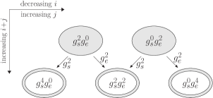
(a) We consider the coupling-power combinations $g_{s}^{i}g_{e}^{j}$ at the amplitude level. From left to right we have increasing $i$ / decreasing $j$ in steps of 2. From top to bottom the total order $i\!+\!j$ increases in steps of 2. The upper row depicts all possible coupling-power combinations for the lowest-order contributions, with $i\!+\!j\!=\!n\!-\!2$, while the lower row depicts all possible coupling-power combinations for the higher-order corrections of one loop order higher, with $i\!+\!j\!=\!n$.

(b) We consider the coupling-power combinations $\alpha_{s}^{x}\alpha_{e}^{y}$ at the squared-amplitude level. From left to right we have increasing $x$ / decreasing $y$ in steps of 1. From top to bottom the total order $x\!+\!y$ increases in steps of 1. The upper row depicts all possible coupling-power combinations for the lowest-order contributions, with $x\!+\!y\!=\!n\!-\!2$, while the lower row depicts all possible coupling-power combinations for the higher-order corrections of one order higher, with $x\!+\!y\!=\!n\!-\!1$.

Figure 1: Coupling-power flow chart for two-parton production at the LHC, for which the lowest-order contributions are defined by tree amplitudes with $n=4$ external particles, at the level of (a) the amplitude and (b) the squared amplitude. See the text for more details.

• At the amplitude level (see Fig. 1(a)), we note that the $g_{s}^{4}g_{e}^{0}$ one-loop contribution is obtained solely from $g_{s}^{2}$ corrections to the $g_{s}^{2}g_{e}^{0}$ lowest-order contribution, and that the $g_{s}^{0}g_{e}^{4}$ one-loop contribution is obtained solely from $g_{e}^{2}$ corrections to the $g_{s}^{0}g_{e}^{2}$ lowest-order contribution. However, the $g_{s}^{2}g_{e}^{2}$ one-loop contribution cannot be classified solely as a QCD or EW one-loop correction to a particular lowest-order contribution, as it contains $g_{s}^{2}$ corrections to $g_{s}^{0}g_{e}^{2}$ and $g_{e}^{2}$ corrections to $g_{s}^{2}g_{e}^{0}$ at the same time, where some of those corrections are being represented by the same diagrams, which do not need to be counted twice. Looking specifically at the four-quark subprocesses of the type $q\bar{q}\rightarrow q^{\prime}\bar{q}^{\prime}$, the two lowest-order contributions are either through gluon exchange or $Z$/$\gamma$ exchange, and for example the one-loop box correction which consists of, say, $qgq^{\prime}Z$ is only generated once, although being at the same time a $g_{s}^{2}$ correction to the lowest-order $Z$/$\gamma$-exchange contribution as well as a $g_{e}^{2}$ correction to the lowest-order gluon-exchange contribution.

• At the squared-amplitude level (see Fig. 1(b)), the possible lowest-order contributions are $\alpha_{s}^{2}\alpha_{e}^{0}$ for all of the subprocesses, as well as $\alpha_{s}^{1}\alpha_{e}^{1}$ and $\alpha_{s}^{0}\alpha_{e}^{2}$ for only the four-quark subprocesses. We note that the $\alpha_{s}^{2}\alpha_{e}^{0}$ lowest-order contributions result solely from squaring the corresponding amplitude-level $g_{s}^{2}g_{e}^{0}$ lowest-order contributions, the order $\alpha_{s}^{0}\alpha_{e}^{2}$ lowest-order contributions results solely from squaring the corresponding amplitude-level $g_{s}^{0}g_{e}^{2}$ lowest-order contributions, while the $\alpha_{s}^{1}\alpha_{e}^{1}$ lowest-order contributions are the result of interfering the amplitude-level contributions of different amplitude-level coupling-power combinations, i.e. interfering the $g_{s}^{2}g_{e}^{0}$ tree diagrams with the $g_{s}^{0}g_{e}^{2}$ tree diagrams consisting of the same external configurations. The one-loop next-to-lowest-order contributions to the contributions in the lower row of Fig. 1(b) are obtained by interfering the contributions from the upper row of Fig. 1(a) with the contributions from the lower row of Fig. 1(a), as formulated generically in Eq. (5). Further note, although the $\alpha_{s}^{1}\alpha_{e}^{1}$ lowest-order contribution, from interfering the lowest-order gluon-exchange and $Z$/$\gamma$-exchange diagrams, is identically zero, due to color arguments, the subset of the $\alpha_{s}^{2}\alpha_{e}^{1}$ one-loop next-to-lowest-order contribution that can be reached from the $\alpha_{s}^{1}\alpha_{e}^{1}$ lowest-order contribution by advancing one power in $\alpha_{s}$ is not zero.

2.3 Renormalization

UV renormalization in NLOX is carried out by means of counterterm (CT) diagrams. Upon generation of diagrams, also all possible CT diagrams are generated, and sorted by coupling powers. The CT diagrams with the same coupling power as a certain set of one-loop diagrams get eventually associated with that set.

The renormalization constants in terms of which the QCD UV counterterms are formulated are derived in a mixed renormalization scheme: a modified on-shell scheme is used for the wave-function and mass renormalization of massive quarks, while the $\overline{\mathrm{MS}}$ scheme is used for massless quarks and gluons, where, however, in the latter case heavy-quark-loop contributions are decoupled by subtracting them at zero momentum [59, 60].

The renormalization constants in terms of which the EW UV counterterms are formulated are derived in the on-shell renormalization scheme as described in Ref. [61] , or, in the presence of potential resonance channels, in the complex-mass scheme [62], where the choice in NLOX is to expand self-energies with complex squared momenta around real squared momenta. As EW input scheme choices NLOX provides both the $\alpha(0)$ and the $G_{\mu}$ EW input schemes [63, 61, 64, 65]. Per default the $\alpha(0)$ EW input scheme is used.

More details are provided in A.

3 Overview on Workflow and Code Generation

NLOX utilizes QGRAF [66], FORM [67, 68], and Python to algebraically generate C++ code for the virtual QCD and EW one-loop contributions to a certain process in terms of one-loop tensor-integral coefficients. The tensor-integral coefficients are calculated recursively at runtime through standard reduction methods by the C++ library TRed, an integral part of NLOX

In this chapter, we give a brief description of how NLOX generates the code and data for a process. As the current release of NLOX contains pre-generated process code and the TRed library, we defer a more complete discussion for a future release of NLOX, which will enable the user to generate process code on their own.

3.1 Algebraic Processing

NLOX begins with text-based model files containing the fields and vertices of the model under consideration. The current version supports the Standard Model with QCD and EW corrections as described in Sec. 2 and A. Such NLOX model is then parsed into a model file for QGRAF [66], which produces a list of diagrams for further processing. Python scripts take the QGRAF output and perform substitutions and simplifications to prepare for further processing by FORM scripts. In this step diagrams of the wrong coupling order, that is those not corresponding to the requested lowest-order or one-loop next-to-lowest-order contributions are discarded. Finally FORM [67, 68] is used to perform further algebraic manipulations and substitutions.

Three main ingredients into the algebraic processing are the treatment of color, the tensor decomposition of one-loop tensor-integrals and the utilization of Standard Matrix Elements, which we will briefly discuss below.

Color Treatment

At the amplitude level, the FORM scripts of NLOX identify the various color structures, i.e. products of color matrices, simplify them, and cache them whilst identifying identical ones, such that only a limited set of unique color strings is kept. At the squared-amplitude level, the various unique color structures are interfered and numerically evaluated, as the interference terms of the various diagrams that contribute to the requested coupling order are evaluated.

Tensor Decomposition

Loop diagrams will contain integrals over the loop momentum. The FORM scripts of NLOX detect these loops, and use a standard decomposition of a tensor integral onto a basis of Lorentz structures [61, 69]. What remains after tensor decomposition are the one-loop tensor-integral coefficients and external momenta of the process. The external momenta are folded into the rest of the diagram, with the tensor coefficients remaining symbolically during script processing, ultimately to be computed at runtime by the tensor-reduction library TRed (see Sec. 4).

Standard Matrix Elements

From a computing standpoint, the most challenging aspect of a diagram-based approach is processing the many gamma matrix expressions that appear in the calculation. To minimize this, strings of gamma matrices (multiplied by momenta and external polarization vectors) in a diagram are brought into a canonical order by anticommutation. Later scripts identify them and reduce the code to unique structures, hence improving efficiency. By an abuse of the standard terminology, we call these unique strings of gamma matrices multiplied by momenta and polarization vectors Standard Matrix Elements (SMEs). After diagram processing, the unique SMEs from a loop or tree amplitude are interfered with the unique (conjugated) SMEs of a tree amplitude. After simplification, a interfered pairs of SMEs, which we will refer to as ISME from here on, can only have uncontracted Lorentz indices within a diagram if the indices belong to different fermion lines. We can safely take all remaining $d$-dimensional indices to be 4-dimensional for SMEs in the HV scheme.. Finally the ISMEs are computed by performing polarization/spin sums and taking traces of the combined strings of gamma matrices (all in 4 dimensions)

At this stage we have color- and helicity-summed expressions stored for each tree or loop diagram interfered with the sum of conjugated tree diagrams, which we call an xdiagram, and which contains references to the ISMEs and to the tensor coefficients in case of loop diagrams, and expressions stored for the ISMEs themselves.

3.2 C++ Code and Process Data Generation

The final stage of process code generation consists of reading the stored analytical xdiagram expressions, and turning them into C++ code to be compiled as well as raw data to be read at runtime. To that end NLOX has a sophisticated Python script to parse FORM output. The script reads xdiagram expressions and ISMEs, and processes the stored expressions. During parsing, any quantity recognized as a variable is identified to be used later in a list of needed variables, to be passed by an interface code. These variables can include constants, couplings, masses, momentum invariants, denominators, and momentum-contracted epsilon tensors. In the case of the latter three, the script generates code to calculate them from momenta and masses. In addition, the list of needed tensor coefficients is compiled.

In one-loop diagrams we must keep terms of $O(\epsilon^{0})$ through $O(\epsilon^{2})$ in case they multiply poles in $\epsilon^{-1}$ or $\epsilon^{-2}$ from the tensor coefficients, resulting in finite pieces. A convenient solution from a C++ coding standpoint is to encapsulate the expression in a class called Poly3 (see B.2), which stores the expression as a three-term polynomial in $\epsilon$.

Turning the FORM output into C++ code directly can result in large code sizes, a disadvantage of using a diagram-based approach, especially in the case of FORM where its strategy is to flatten expressions to many small terms to be processed serially. However, the advantage of the approach is that the expressions produced are very regular. As such, we have implemented options for turning these regular expressions into data stored in text files, to be read at run time. Their computation then requires only simple loops over many terms, both for the diagrams and ISMEs. Many identical expressions are also identified at this stage. In our current release we only support producing processes that have been turned to data to the full extent possible. Not only does this reduce code size, but it results in much faster code.

The final result is a small C++ code that computes with the following steps:

• Pass to the process the variables it needs, namely constants, couplings, masses, and momenta for a given phase-space point (PSP).

• Calculate the ISMEs, whose results are stored in an array to be retrieved by the xdiagram calculating code.

• Calculate the needed tensor coefficients, which we call TIs, stored in a TRed object (see Sec. 4).

• For each xdiagram, calculate the result, using the ISME and tensor coefficient results as input. Schematically these calculations are loops summing prefactor*ISME*TI, where each prefactor contains all the dependence of the diagram that is not an ISME or tensor coefficient, usually couplings, masses, and momentum invariants.

4 Tensor Reduction and the TRed library

The tensor-integral coefficients (see Sec. 3.2), in terms of which the C++ code for the virtual contributions to a particular process is expressed, are calculated recursively at runtime by the C++ library TRed. Several reduction techniques are available to TRed, many of which are found in Refs. [71, 69, 72]. From here on we use TRed interchangeably to refer either to the tensor-reduction library TRed or an object of the TRed class (see B.1).

TRed accumulates and stores a list of all tensor coefficients which appear during the recursion and are needed by a particular process, along with their dependencies. Only needed coefficients are computed, and no coefficient is computed more than once, making the reduction process particularly efficient. The coefficient values are returned as Poly3 (see B.2).

4.1 Functionality of TRed

As mentioned in Sec. 3.1, tensor integrals appearing in Feynman diagrams are identified and tensor decomposed during diagram processing by FORM scripts. The tensor coefficients appearing in this expansion are identified in Python scripts during source code generation, and a list of needed coefficients is accumulated. This list is loaded at runtime, and one-by-one a tensor coefficient is requested of TRed. Each created tensor coefficient is stored in TRed, and a pointer returned to the calling process for later retrieval of its value.

Many schemes to reduce tensor one-loop integrals to combinations of known scalar one-loop integrals have been described in the literature. One approach to implement these schemes would be to compute the tensor coefficients analytically and code the result into a library. Not even accounting for the different kinematic limits of each tensor coefficient, this would require hundreds of coded functions just to cover 5-point integrals. However, it may be more efficient and general to do this numerically at run-time by coding the functions that determine one coefficient from others, which is the approach that TRed take, thereby implementing several traditional reduction schemes, many of which are found in Refs. [71, 69, 72].

The dependencies of a given coefficient are different depending on the chosen reduction method. Multiple methods, some overlapping, are implemented in TRed. When a coefficient is requested during process initialization, the following steps are taken:

• Check whether the coefficient is already stored. If so, just return a pointer to it. If not, build a new coefficient.

• If a new coefficient is needed, for each active reduction method, determine the new coefficient’s dependencies. If a dependency already exists, create and store a pointer to it for use by the new coefficient. If not, create that coefficient, and so on, recursively.

Eventually for a given method and requested coefficient, this process will terminate with coefficients that can be computed directly, usually a scalar coefficient. This process guarantees that all needed coefficients are available, but no unneeded coefficients are ever created or computed. The coefficient objects (and pointers to dependencies) are created once at runtime. From there, TRed is given a PSP and asked to evaluate its stored coefficients. In NLOX a process then is computed at that PSP using these coefficient values as input.

The scalar integrals that stand at the end of the recursions are not computed by the TRed library, as many libraries are already available. Rather, interfaces to several external scalar libraries are available in TRed: QCDLoop  1 [73] and 2 [74], LoopTools [75], and OneLOop [76]. In its current version the NLOX package, provided through the NLOX_util collection of necessary dependencies, contains QCDLoop  1.95 and OneLOop 3.6 by default.

4.2 Features of TRed

Multiple Reduction Methods

As of this note, the following reduction methods are implemented and used in TRed:

• 1- and 2-point integrals ($A$ and $B$ coefficients): Rather than use a standard reduction, these are computed directly, without numerical recursion, using the analytical formulas of Ref. [69]. However, in the current implementation of the Standard Model used by NLOX and reduction methods available for higher-point integrals, the only $A$ coefficients appearing in the reduction are scalars and the higher-rank $A$ coefficients are not used.

• 3- and 4-point integrals ($C$ and $D$ coefficients): Two reduction methods are implemented, Passarino-Veltman (PV) [71] and an alternate, similar reduction of Denner and Dittmaier (DD) [69], that uses modified Cayley matrices instead of Gram matrices. As the Cayley matrices are singular when there are IR singularities, TRed requires that PV be available, and when such a singularity is detected TRed will disable the DD node and revert to PV. PV alone is enabled by default.

• 5- and 6-point integrals ($E$ and $F$ coefficients): These types of nodes are different in that their reductions make use of the fact that only four independent momenta are needed to span a 4-dimensional spacetime. Two reduction methods are implemented, one by Diakonidis et. al. [72], and one by Denner and Dittmaier [69]. As the former method is limited to rank 3 integrals, we use the latter by default.

The TRed source code is extensible to other methods without much modification beyond the actual implementation of the method, and we anticipate adding others in the future.

Stability Checks and Higher Precision

$\epsilon$-pole parts of tensor coefficients tend to be much simpler analytically than their corresponding finite parts. This is especially true for IR-finite coefficients. A library of coefficients with UV-only divergences exists inside TRed for the purposes of comparing to values determined by the numerical reduction method – this code is simple and fast, so it can be used to check the numerical reduction without significant effect on the runtime. If a given coefficient fails to match within a certain threshold, it and all its dependencies are recomputed at a higher floating-point precision level automatically. Three precision levels are attempted: double precision (64-bit), long double precision (80-bit on typical modern machines) and finally 128-bit (implemented by the quadmath library). In addition, it is possible to request all coefficients at a higher precision by requesting evaluation from TRed again before feeding a new PSP, which may be useful if further checks are done at the level of an interfaced process, where for instance the poles of a renormalized virtual and real process are checked for cancellation. If, after recomputation at the highest set floating-point precision, a given coefficient still fails to match within a certain precision, the one-loop contribution in question at the PSP in question is deemed inaccurate, and TRed returns a corresponding flag.

Kinematics Cache

Invariants and various matrices, determinants, etc. are used (and reused) during the numerical reduction. Rather than constantly recompute them, for each PSP they are computed on first request and stored for future use. The cache is cleared when the PSP is updated.

5 Using NLOX

To access the host URL for the NLOX package, please go to http://www.hep.fsu.edu/~nlox. For further details on downloading and using NLOX, beyond what is described in the section at hand, please follow the instructions on the website.

5.1 Components of the NLOX package

The current release of the NLOX package contains the following.

• NLOX: This first public release of NLOX consists of the TRed library, as well as the functionality to interface process archives, containing already generated process code.

• NLOX_util: Scalar integrals are not computed by the TRed library, as many libraries are already available. Rather, interfaces to external scalar libraries are available. QCDLoop  1 [73] and OneLOop [76] are the current default and are in this release of the NLOX package provided through the NLOX_util collection of necessary dependencies, containing QCDLoop  1.95 and OneLOop 3.6.

• Process archives: Currently, already generated process code is provided through process archives, i.e. tarballs containing pre-generated process code.

A simple set of instructions on how to download and install the various components can be found on http://www.hep.fsu.edu/~nlox.

5.2 Interfacing Processes

NLOX computes the lowest-order and one-loop next-to-lowest-order contributions to a certain subprocess at the level of the UV renormalized, color- and helicity-summed squared amplitude and returns the values for the Laurent coefficients defined in Eqs. (6) and (7), which we briefly repeat :

$$g_{s}^{i^{\prime}\!\!+i}g_{e}^{2(n-2)-i^{\prime}\!\!-i}\left(A_{n}^{(0)(i^{\prime})}\right)^{\!*}\!\left(A_{n}^{(0)(i)}\right) \,=\;a_{0}^{(i^{\prime}\!,i)}\;+\;\mathcal{O}(\epsilon)\,,$$ (8)

$$g_{s}^{i^{\prime}\!\!+i}g_{e}^{2(n-1)-i^{\prime}\!\!-i}\,2\,\mathrm{Re}\left(\left(A_{n}^{(0)(i^{\prime})}\right)^{\!*}\!\left(A_{n}^{(1)(i)}\right)\right) \,=\;S_{\epsilon}\,\bigg{(}\frac{c_{2}^{(i^{\prime}\!,i)}}{\epsilon^{2}}+\frac{c_{1}^{(i^{\prime}\!,i)}}{\epsilon}+c_{0}^{(i^{\prime}\!,i)}\bigg{)}\;+\;\mathcal{O}(\epsilon)\,,$$ (9)

with $S_{\epsilon}=(4\pi)^{\epsilon}/\Gamma(1-\epsilon)$. Given a process, of which the lowest-order contributions are defined by tree amplitudes with $n$ external particles, in terms of an expansion in $\alpha_{s}^{x}\alpha_{e}^{y}$, for a particular lowest-order Laurent coefficient $a_{0}^{(i^{\prime}\!,i)}$ with a combined power $(i^{\prime}\!\!+\!i)=2x$ of $g_{s}$ in the tree${}^{*}\!$/tree interference we read off the combined power of $g_{e}$ to be $2y=(j^{\prime}\!\!+\!j)=2(n\!-\!2)\!-\!(i^{\prime}\!\!+\!i)$, whereas for a particular one-loop next-to-lowest-order Laurent coefficient $c_{\epsilon}^{(i^{\prime}\!,i)}$ with a combined power $(i^{\prime}\!\!+\!i)=2x$ of $g_{s}$ in the tree${}^{*}\!$/one-loop interference we read off the combined power of $g_{e}$ to be $2y=(j^{\prime}\!\!+\!j)=2(n\!-\!1)\!-\!(i^{\prime}\!\!+\!i)$.

Once NLOX and NLOX_util are installed, and the libraries in the process archive for the process under consideration are compiled (see previous section),

• the only file that needs to be included in the users main program is nlox_olp.h for a C++ program and nlox_fortran_interface.f90 for a Fortran program,

• the value for a particular lowest-order or next-to-lowest-order Laurent coefficient of a particular subprocess can be retrieved by the function NLOX_OLP_EvalSubProcess(). This function is based on the standard BLHA [18], with additional arguments to select the desired power of couplings.

In a C++ program we have

• NLOX_OLP_EvalSubProcess(&isub, typ, cp, pp, &next, &mu, rval2, &acc)

with

• isub: Integer number specifying the ID of the subprocess in question.

• typ: Character string specifying the interference type, i.e. either "tree_tree" or "tree_loop" (note the double quotes).

• cp: Character string specifying the coupling power of the interference type in question, in the format "g$i^{\prime}$e$j^{\prime}$_g$i$e$j$". For example, for $u\bar{u}\rightarrow t\bar{t}$ the interference of the tree amplitude with the highest possible $g_{s}$ power of 2 (and a complementing $g_{e}$ power of 0) with the one-loop amplitude with the highest possible $g_{s}$ power of 4 (and a complementing $g_{e}$ power of 0) has cp="g2e0_g4e0".

  • For a particular isub and a particular typ, there are potentially multiple values of cp that contribute to the same coupling power at the squared-amplitude level, i.e. in terms of an expansion in $\alpha_{s}^{x}\alpha_{e}^{y}=\alpha_{s}^{(i^{\prime}\!+i)/2}\alpha_{e}^{(j^{\prime}\!+j)/2}$. For typ="tree_loop" they need to be retrieved separately and summed, e.g. cp="g2e0_g2e2" and cp="g0e2_g4e0" for $u\bar{u}\rightarrow t\bar{t}$. For typ="tree_tree" each yields the same result, e.g. cp="g2e0_g0e2" or cp="g0e2_g2e0" for $u\bar{u}\rightarrow t\bar{t}$.

  • All available values for isub, typ and cp, for a particular process in question, are listed in the SUBPROCESSES file in the corresponding process archive.

• mu: Double precision number specifying the scale, in units of GeV.

• next: Integer determining the number of external particles of the subprocess in question.

• pp: Array of double precision numbers, with dimension $5\cdot\texttt{next}$, which specifies the PSP $\{p_{1},p_{2}\}\rightarrow\{p_{3},...,p_{\texttt{next}}\}$, in units of GeV, and is of the form pp = [ $p_{1,t}$ , $p_{1,x}$ , $p_{1,y}$ , $p_{1,z}$ , $m_{1}$ , $p_{2,t}$ , $p_{2,x}$ , ... ].

• rval2: Returned array of double precision numbers, with dimension 3, which contains the results for the Laurent coefficients of order $(i^{\prime}\!,i)$ in Eqs. (8) and (9), evaluated at pp, and

  • for typ = "tree_tree" is of the form rval2[0,1,2] = [$\,0\,$,$\,0\,$,$\,a_{0}^{(i^{*}\!,i)}\,$],

  • for typ = "tree_loop" is of the form rval2[0,1,2] = [$\,c_{2}^{(i^{*}\!,i)}$, $c_{1}^{(i^{*}\!,i)}$, $c_{0}^{(i^{*}\!,i)}\,$].

• acc: Always reports the integer 0 in this release.

In a Fortran program we have

• NLOX_OLP_EvalSubProcess(isub, typ, ltyp, cp, lcp, pp, next, mu, rval2, acc)

where

• in addition to the above there are two additional arguments, ltyp and lcp, i.e. integer numbers specifying the number of characters in the character strings typ (always ltyp=9) and cp (most likely always lcp=9) respectively. Where arrays in C++ start with element 0, arrays in Fortran start with element 1: pp[0,1,...,5$\cdot$next-1]$\rightarrow$pp(1,2,...,5$\cdot$next) and rval2[0,1,2]$\rightarrow$rval2(1,2,3).

A simple set of instructions on how to interface to the process archives, which further point to the example programs that are currently provided with each process archive, can be found on http://www.hep.fsu.edu/~nlox.

6 Benchmarks

In this section we compare PSP results of NLOX for selected processes against another program, Recola [6]. Comparisons to other codes can be found in [77]. In addition to serving as a useful check, this section can serve as a useful reference for those attempting to test the installation and use of a process archive. We also give NLOX time benchmarks for each of the processes in this section.

6.1 General Setup

The results presented in this section are obtained calculating EW corrections using the complex mass scheme and defining renormalized EW parameters in the $\alpha(0)$ input scheme (see Sect. 2.3 and A.2). All particles have zero width unless otherwise specified. We use a diagonal CKM matrix. All leptons and the four lightest quarks are considered massless, and all other parameters are listed in Table 1. Their values are arbitrarily chosen just for the sake of benchmarking, and correspond to values used e.g. already in [77] to compare with other packages such as GoSam (see Ref. [77] for more details). The same setup is also used as NLOX default setup, and will have to be adapted to specific calculations as needed by modifying the choice of input parameters as further explained on http://www.hep.fsu.edu/~nlox.

$\alpha$	1	$\alpha_{s}$	1
$m_{b}$	4.2 GeV	$m_{t}$	171.2 GeV
$m_{W}$	80.376 GeV	$m_{Z}$	91.1876 GeV
$m_{H}$	125 GeV	$\mu$	1000 GeV

Table 1: Input values used in this chapter’s comparisons, and the defaults for NLOX.

For simplicity we test all processes with a common set of PSPs, obtained for a center-of-mass energy $\sqrt{s}=1$ TeV. For a given multiplicity, these PSPs only depend on the masses of the external particles. We list them in Tables 6 through 12 of C. According to Table 1, the renormalization scale is also chosen to be $\mu=1$ TeV.

6.2 Processes

For all processes, we report PSP results for all or part of the individual channels contributing to the process in terms of the Laurent coefficients of the expansions in Eqs. (6)/(8) and (7)/(9). As explained above, given a process, of which the lowest-order contributions are defined by tree amplitudes with $n$ external particles, in terms of an expansion in $\alpha_{s}^{x}\alpha_{e}^{y}$, for a particular lowest-order Laurent coefficient $a_{0}^{(i^{\prime}\!,i)}$ with a combined power $(i^{\prime}\!\!+\!i)=2x$ of $g_{s}$ in the tree${}^{*}\!$/tree interference we read off the combined power of $g_{e}$ to be $2y=(j^{\prime}\!\!+\!j)=2(n\!-\!2)\!-\!(i^{\prime}\!\!+\!i)$, whereas for a particular one-loop next-to-lowest-order Laurent coefficient $c_{\epsilon}^{(i^{\prime}\!,i)}$ with a combined power $(i^{\prime}\!\!+\!i)=2x$ of $g_{s}$ in the tree${}^{*}\!$/one-loop interference we read off the combined power of $g_{e}$ to be $2y=(j^{\prime}\!\!+\!j)=2(n\!-\!1)\!-\!(i^{\prime}\!\!+\!i)$.

Note that for each coupling-power combination $(i^{\prime}\!,i)$ the evaluation time for each associated Laurent coefficient is the same, as they are retrieved simultaneously through TRed’s Poly3 construct.

In the following benchmark results, we will not print those that are identically zero throughout all $\epsilon$ due to symmetry considerations (e.g. due to color arguments; we make an exception in the following for $u\bar{u}\rightarrow t\bar{t}$, though, as an example), and in general we will not give all possible power-coupling combinations. We also refrain from giving results for every subprocess, although they have been generated and are available in the process repository, allowing also for massive initial-state $b$ quarks if applicable.

All results are computed using OneLOop as the scalar provider, since it allows the option of complex mass arguments, needed if widths are used.

6.2.1 $pp\rightarrow t\bar{t}$

In the case of massless initial-state particles this process consists of three independent subprocesses: $u\bar{u}\rightarrow t\bar{t}$, $d\bar{d}\rightarrow t\bar{t}$, and $gg\rightarrow t\bar{t}$, all tested with the PSP of Table 6. In our process archive we also provide a distinct initial state for the $b$-quark channel, in case of a massive $b$ quark. The fixed-order NLO QCD corrections to $pp\rightarrow t\bar{t}$ were first calculated in [60, 78, 79, 80], while the corresponding NLO EW corrections can be found in [81, 82, 83, 84, 85, 86, 87, 88].

To give an example, for the quark-initiated subprocesses the complete set of lowest-order contributions is ($a_{0}^{(i^{\prime},i)}\,\widehat{=}\,$ tree_tree g$i^{\prime}$e$j^{\prime}$_g$i$e$j$, with $j^{\prime}=n-2-i^{\prime}$, $j=n-2-i$ and $n=4$)

• $a_{0}^{(2,2)}\,\widehat{=}\,$ tree_tree g2e0_g2e0, $a_{0}^{(2,0)}\!=\!a_{0}^{(0,2)}\,\widehat{=}\,$ tree_tree g2e0_g0e2 = tree_tree g0e2_g2e0, $a_{0}^{(0,0)}\,\widehat{=}\,$ tree_tree g0e2_g0e2,

while the complete set of next-to-lowest-order contributions is ($c_{\epsilon}^{(i^{\prime},i)}\,\widehat{=}\,$ tree_loop g$i^{\prime}$e$j^{\prime}$_g$i$e$j$, with $j^{\prime}=n-2-i^{\prime}$, $j=n-i$ and $n=4$)

• $c_{\epsilon}^{(2,4)}\,\widehat{=}\,$ tree_loop g2e0_g4e0, $c_{\epsilon}^{(2,2)}\,\widehat{=}\,$ tree_loop g2e0_g2e2, $c_{\epsilon}^{(2,0)}\,\widehat{=}\,$ tree_loop g2e0_g0e4, $c_{\epsilon}^{(0,4)}\,\widehat{=}\,$ tree_loop g0e2_g4e0, $c_{\epsilon}^{(0,2)}\,\widehat{=}\,$ tree_loop g0e2_g2e2, $c_{\epsilon}^{(0,0)}\,\widehat{=}\,$ tree_loop g0e2_g0e4.

The following contributions are identically zero throughout all $\epsilon$, though, due to color arguments (always producing a color trace over only one fundamental color matrix): $a_{0}^{(2,0)}=a_{0}^{(0,2)}$ and $c_{\epsilon}^{(2,0)}$. For the gluon-initiated subprocess we only have $a_{0}^{(2,2)}$, $c_{\epsilon}^{(2,4)}$ and $c_{\epsilon}^{(2,2)}$, none of them being identically zero throughout all $\epsilon$ (e.g. due to color arguments; the $\mathcal{O}(\alpha_{s}^{2}\alpha_{e}^{1})$ contribution has no double pole, though). More details in regards to the coupling-power picture for this process (and also the process $pp\rightarrow jj$; see next section) are given in the example at the end of Sec. 2.2.

$u\bar{u}\rightarrow t\bar{t}$		NLOX	Recola
$\mathcal{O}(\alpha_{s}^{2}\alpha_{e}^{0})$	$a_{0}^{(2,2)}$	69.83600143751471	69.83600143751464
$\mathcal{O}(\alpha_{s}^{1}\alpha_{e}^{1})$	$a_{0}^{(2,0)}$	0	0
	$a_{0}^{(0,2)}$	0	0
$\mathcal{O}(\alpha_{s}^{0}\alpha_{e}^{2})$	$a_{0}^{(0,0)}$	8.373783006235811	8.373783006235795
$\mathcal{O}(\alpha_{s}^{3}\alpha_{e}^{0})$	$c_{2}^{(2,4)}$	-29.63931955881074	-29.63931955869816
	$c_{1}^{(2,4)}$	-21.62010557945776	-21.62010557948297
	$c_{0}^{(2,4)}$	326.7316251339323	326.7316251338464
$\mathcal{O}(\alpha_{s}^{2}\alpha_{e}^{1})$	$c_{2}^{(2,2)}$	-9.879773186270731	-9.879773186033162
	$c_{1}^{(2,2)}$	100.9206592499375	100.9206592501215
	$c_{0}^{(2,2)}$	-264.008143628928	-264.0081436286176
$\mathcal{O}(\alpha_{s}^{2}\alpha_{e}^{1})$	$c_{2}^{(0,4)}$	-3.016507999556917e-13	3.632294465205632e-11
	$c_{1}^{(0,4)}$	24.46218467653051	24.46218467654894
	$c_{0}^{(0,4)}$	40.71710556011429	40.71710556012410
$\mathcal{O}(\alpha_{s}^{1}\alpha_{e}^{2})$	$c_{2}^{(2,0)}$	0	5.797831350820261e-16
	$c_{1}^{(2,0)}$	0	1.627710312214327e-14
	$c_{0}^{(2,0)}$	0	-7.232455052854060e-15
$\mathcal{O}(\alpha_{s}^{1}\alpha_{e}^{2})$	$c_{2}^{(0,2)}$	-3.553943887523572	-3.553943887523602
	$c_{1}^{(0,2)}$	3.465847464830842	3.465847464830841
	$c_{0}^{(0,2)}$	44.3414894585291	44.34148945852903
$\mathcal{O}(\alpha_{s}^{0}\alpha_{e}^{3})$	$c_{2}^{(0,0)}$	-1.184647962507978	-1.184647962463359
	$c_{1}^{(0,0)}$	-2.08629577374953	-2.086295773705025
	$c_{0}^{(0,0)}$	-46.41633996223131	-46.41633996214514

Table 2: $u\bar{u}\rightarrow t\bar{t}$. The following contributions are identically zero throughout all $\epsilon$, due to color arguments: $a_{0}^{(2,0)}=a_{0}^{(0,2)}$, $c_{\epsilon}^{(2,0)}$.

$d\bar{d}\rightarrow t\bar{t}$		NLOX	Recola
$\mathcal{O}(\alpha_{s}^{2}\alpha_{e}^{0})$	$a_{0}^{(2,2)}$	69.83600143751471	69.83600143751464
$\mathcal{O}(\alpha_{s}^{0}\alpha_{e}^{2})$	$a_{0}^{(0,0)}$	2.807482983131919	2.807482983131935
$\mathcal{O}(\alpha_{s}^{3}\alpha_{e}^{0})$	$c_{2}^{(2,4)}$	-29.63931955881074	-29.63931955869816
	$c_{1}^{(2,4)}$	-21.62010557945776	-21.62010557948297
	$c_{0}^{(2,4)}$	326.7316251339323	326.7316251338464
$\mathcal{O}(\alpha_{s}^{2}\alpha_{e}^{1})$	$c_{2}^{(2,2)}$	-2.46994329656692	-2.469943296594337
	$c_{1}^{(2,2)}$	-10.30104753296668	-10.30104753304126
	$c_{0}^{(2,2)}$	-876.7537677581068	-876.7537677580882
$\mathcal{O}(\alpha_{s}^{2}\alpha_{e}^{1})$	$c_{2}^{(0,4)}$	-5.255491264144508e-14	1.550315431586569e-12
	$c_{1}^{(0,4)}$	2.361140127198419	2.361140127198432
	$c_{0}^{(0,4)}$	3.873233073210399	3.873233073210025
$\mathcal{O}(\alpha_{s}^{1}\alpha_{e}^{2})$	$c_{2}^{(0,2)}$	-1.191532785098194	-1.191532785098204
	$c_{1}^{(0,2)}$	1.161996647440871	1.161996647440898
	$c_{0}^{(0,2)}$	17.55679660782326	17.55679660782354
$\mathcal{O}(\alpha_{s}^{0}\alpha_{e}^{3})$	$c_{2}^{(0,0)}$	-0.09929439875817378	-0.09929439875884327
	$c_{1}^{(0,0)}$	-4.282220826752567	-4.282220826748949
	$c_{0}^{(0,0)}$	-48.01638812955415	-48.01638812949420

Table 3: $d\bar{d}\rightarrow t\bar{t}$. The following contributions are identically zero throughout all $\epsilon$, due to color arguments: $a_{0}^{(2,0)}=a_{0}^{(0,2)}$, $c_{\epsilon}^{(2,0)}$.

$gg\rightarrow t\bar{t}$		NLOX	Recola
$\mathcal{O}(\alpha_{s}^{2}\alpha_{e}^{0})$	$a_{0}^{(2,2)}$	726.898367145306	726.8983671453062
$\mathcal{O}(\alpha_{s}^{3}\alpha_{e}^{0})$	$c_{2}^{(2,4)}$	-694.1368095396184	-694.1368095396263
	$c_{1}^{(2,4)}$	-2548.515434412368	-2548.515434412614
	$c_{0}^{(2,4)}$	-429.2152536196467	-429.2152536220427
$\mathcal{O}(\alpha_{s}^{2}\alpha_{e}^{1})$	$c_{2}^{(2,2)}$	0	0.000000000000000
	$c_{1}^{(2,2)}$	254.5385946968528	254.5385946969382
	$c_{0}^{(2,2)}$	523.671501813473	523.6715018106897

Table 4: $gg\rightarrow t\bar{t}$.

6.2.2 $pp\rightarrow jj$

Fixed-order NLO QCD corrections to $pp\rightarrow jj$ were first calculated in [89], while the corresponding NLO EW corrections can be found in [90]. With electroweak corrections included, this process contains 37 numerically distinct subprocesses, including $b$ jets in the final state and $b$ quarks in the initial state, which are distinct if the $b$ quarks are massive. This count takes into account symmetries that produce identical subprocess code. We present a few representative comparisons here for the entirely massless 2-to-2 PSP in Table 7.

More details in regards to the coupling-power picture for this process (and also the process $pp\rightarrow t\bar{t}$; see previous section) are given in the example at the end of Sec. 2.2.

$u\bar{u}\rightarrow d\bar{d}$		NLOX	Recola
$\mathcal{O}(\alpha_{s}^{2}\alpha_{e}^{0})$	$a_{0}^{(2,2)}$	69.78980394856457	69.78980394856457
$\mathcal{O}(\alpha_{s}^{1}\alpha_{e}^{1})$	$a_{0}^{(2,0)}$	-0.001242222784080782	-0.001242222784081074
	$a_{0}^{(0,2)}$	-0.001242222784080782	-0.001242222784081074
$\mathcal{O}(\alpha_{s}^{3}\alpha_{e}^{0})$	$c_{2}^{(2,4)}$	-59.239425471085	-59.23942547109301
	$c_{1}^{(2,4)}$	-175.9794797288048	-175.9794797287917
	$c_{0}^{(2,4)}$	-98.41451624298804	-98.41451624298804
$\mathcal{O}(\alpha_{s}^{2}\alpha_{e}^{1})$	$c_{2}^{(2,2)}$	-12.34049254169433	-12.34049254170276
	$c_{1}^{(2,2)}$	-66.57794605840587	-66.57794605839047
	$c_{0}^{(2,2)}$	-641.7235774288396	-641.7235774288340
$\mathcal{O}(\alpha_{s}^{2}\alpha_{e}^{1})$	$c_{2}^{(0,4)}$	0.001054431448151187	0.001054431447901294
	$c_{1}^{(0,4)}$	9.889347931105585	9.889347931106062
	$c_{0}^{(0,4)}$	19.48443223966789	19.48443223965836
$dg\rightarrow dg$		NLOX	Recola
$\mathcal{O}(\alpha_{s}^{2}\alpha_{e}^{0})$	$a_{0}^{(2,2)}$	25089.40333374167	25089.40333374156
$\mathcal{O}(\alpha_{s}^{3}\alpha_{e}^{0})$	$c_{2}^{(2,4)}$	-34606.88885152432	-34606.88885153094
	$c_{1}^{(2,4)}$	-189987.7760195865	-189987.7760195137
	$c_{0}^{(2,4)}$	-308102.3176212214	-308102.3176212332
$\mathcal{O}(\alpha_{s}^{2}\alpha_{e}^{1})$	$c_{2}^{(2,2)}$	-887.3561243980364	-887.3561243987060
	$c_{1}^{(2,2)}$	-1333.535787238849	-1333.535787235778
	$c_{0}^{(2,2)}$	-5924.964392741716	-5924.964392718713
$gg\rightarrow gg$		NLOX	Recola
$\mathcal{O}(\alpha_{s}^{2}\alpha_{e}^{0})$	$a_{0}^{(2,2)}$	44706663.18826243	44706663.18826232
$\mathcal{O}(\alpha_{s}^{3}\alpha_{e}^{0})$	$c_{2}^{(2,4)}$	-85383437.22667754	-85383437.22669885
	$c_{1}^{(2,4)}$	-369364175.5404882	-369364175.5404322
	$c_{0}^{(2,4)}$	-281755147.8249173	-281755147.8249879

6.2.3 $pp\rightarrow Zb$

This process was examined by the authors using NLOX recently [52, 53], where particular attention was paid to EW corrections and using a massive $b$ quark. The corresponding fixed-order NLO QCD corrections were first calculated in [91].

This process proceeds through only one channel, $bg\rightarrow Zb$. We present the case of a massive $b$, with the PSP given in Tab. 8.

$bg\rightarrow Zb$		NLOX	Recola
$\mathcal{O}(\alpha_{s}^{1}\alpha_{e}^{1})$	$a_{0}^{(1,1)}$	56.70705366755421	56.70705366755446
$\mathcal{O}(\alpha_{s}^{2}\alpha_{e}^{1})$	$c_{2}^{(1,3)}$	-27.07562369811053	-27.07562369824791
	$c_{1}^{(1,3)}$	219.1031319518903	219.1031319535024
	$c_{0}^{(1,3)}$	1719.562951862683	1719.562951868557
$\mathcal{O}(\alpha_{s}^{1}\alpha_{e}^{2})$	$c_{2}^{(1,1)}$	0	0.000000000000000
	$c_{1}^{(1,1)}$	-29.9292665465376	-29.92926654654536
	$c_{0}^{(1,1)}$	-1381.341046035739	-1381.341046280566

6.2.4 $pp\rightarrow e^{+}e^{-}$

To provide a simple test of the complex mass scheme, we examine the Drell-Yan process mediated both by a photon, and, in contrast to other tests in this section, by a $Z$ with its width. For this process only, the parameters $m_{Z}=91.1534806191828$ and $\Gamma_{Z}=2.49426637877282$ (GeV) are used, with all other parameters as in Tab. 1. In the following we give results for the $u\bar{u}\rightarrow e^{+}e^{-}$ channel, using the PSP of Tab. 7. Fixed-order NLO QCD corrections to the Drell-Yan process were first calculated in [92], while NLO EW corrections for the neutral current Drell-Yan process can be found in [93, 94].

$u\bar{u}\rightarrow e^{+}e^{-}$		NLOX	Recola
$\mathcal{O}(\alpha_{s}^{0}\alpha_{e}^{2})$	$a_{0}^{(0,0)}$	117.4358832604318	117.4358832604319
$\mathcal{O}(\alpha_{s}^{1}\alpha_{e}^{2})$	$c_{2}^{(0,2)}$	-49.84133684602794	-49.84133684602804
	$c_{1}^{(0,2)}$	-74.76200526904191	-74.76200526904215
	$c_{0}^{(0,2)}$	46.59179136175548	46.59179136175552
$\mathcal{O}(\alpha_{s}^{0}\alpha_{e}^{3})$	$c_{2}^{(0,0)}$	-53.99478158319884	-53.99478158322654
	$c_{1}^{(0,0)}$	53.74087481152656	53.74087481148945
	$c_{0}^{(0,0)}$	-2951.1335231532	-2951.133523154139

6.2.5 $e^{+}e^{-}\rightarrow ht\bar{t}$

As an example of a lepton-initiated process, we present $e^{+}e^{-}\rightarrow ht\bar{t}$. It uses the PSP given in Tab. 9. Fixed-order NLO QCD corrections for this process have been calculated in [95, 96], while the corresponding NLO EW corrections have been presented in [97, 98, 99].

$e^{+}e^{-}\rightarrow ht\bar{t}$		NLOX	Recola
$\mathcal{O}(\alpha_{s}^{0}\alpha_{e}^{3})$	$a_{0}^{(0,0)}$	0.1650875547906978	0.1650875547906976
$\mathcal{O}(\alpha_{s}^{1}\alpha_{e}^{3})$	$c_{2}^{(0,2)}$	0	0.000000000000000
	$c_{1}^{(0,2)}$	0.04539059879996656	0.04539059879996588
	$c_{0}^{(0,2)}$	0.4149530650547262	0.4149530650547257
$\mathcal{O}(\alpha_{s}^{0}\alpha_{e}^{4})$	$c_{2}^{(0,0)}$	-0.05254900077578735	-0.05254900077578772
	$c_{1}^{(0,0)}$	-0.4184851162495272	-0.4184851162495317
	$c_{0}^{(0,0)}$	-5.119506322697255	-5.119506321326591

6.2.6 $pp\rightarrow Zt\bar{t}$

This process has three (four) distinct subprocesses if the initial state $b$ is treated as massless (massive). In the following we give benchmark results for the $u\bar{u}\rightarrow Zt\bar{t}$ and $gg\rightarrow Zt\bar{t}$ channels, using the PSP of Tab. 10. Fixed-order NLO QCD corrections for this process have been calculated in [100, 101, 102, 103, 104], while the corresponding NLO EW corrections have been presented in [41].

$u\bar{u}\rightarrow Zt\bar{t}$		NLOX	Recola
$\mathcal{O}(\alpha_{s}^{2}\alpha_{e}^{1})$	$a_{0}^{(2,2)}$	0.02418281962609314	0.02418281962609323
$\mathcal{O}(\alpha_{s}^{3}\alpha_{e}^{1})$	$c_{2}^{(2,4)}$	-0.01026350741704608	-0.01026350741704629
	$c_{1}^{(2,4)}$	-0.01772187646503733	-0.01772187646503737
	$c_{0}^{(2,4)}$	0.1034156002235128	0.1034156002235174
$\mathcal{O}(\alpha_{s}^{2}\alpha_{e}^{2})$	$c_{2}^{(2,2)}$	-0.003421169139015138	-0.003421169139015495
	$c_{1}^{(2,2)}$	-0.02453440885384433	-0.02453440885384411
	$c_{0}^{(2,2)}$	-0.3832664778286854	-0.3832664783495138
$\mathcal{O}(\alpha_{s}^{2}\alpha_{e}^{2})$	$c_{2}^{(0,4)}$	1.834978622567579e-16	6.418476861114186e-17
	$c_{1}^{(0,4)}$	-0.003287144564297587	-0.003287144564297309
	$c_{0}^{(0,4)}$	-0.006365140215048126	-0.006365140215044396
$gg\rightarrow Zt\bar{t}$		NLOX	Recola
$\mathcal{O}(\alpha_{s}^{2}\alpha_{e}^{1})$	$a_{0}^{(2,2)}$	0.01377970228330338	0.01377970228330350
$\mathcal{O}(\alpha_{s}^{3}\alpha_{e}^{1})$	$c_{2}^{(2,4)}$	-0.0131586463963351	-0.01315864639633449
	$c_{1}^{(2,4)}$	-0.0189899781008642	-0.01898997810086434
	$c_{0}^{(2,4)}$	0.05073427513231134	0.05073427513231166
$\mathcal{O}(\alpha_{s}^{2}\alpha_{e}^{2})$	$c_{2}^{(2,2)}$	0	0.000000000000000
	$c_{1}^{(2,2)}$	-0.007929673919194006	-0.007929673919193275
	$c_{0}^{(2,2)}$	-0.162870316537v5728	-0.1628703165354349

6.2.7 $pp\rightarrow W^{+}t\bar{t}$

This process proceeds through only one distinct channel. The following results are obtained using the PSP in Table 11. Fixed-order NLO QCD corrections for this process have been calculated in [105, 103, 104], while the corresponding NLO EW corrections have been presented in [41, 51].

$u\bar{d}\rightarrow W^{+}t\bar{t}$		NLOX	Recola
$\mathcal{O}(\alpha_{s}^{2}\alpha_{e}^{1})$	$a_{0}^{(2,2)}$	0.03893217777719004	0.03893217777718989
$\mathcal{O}(\alpha_{s}^{3}\alpha_{e}^{1})$	$c_{2}^{(2,4)}$	-0.01652332943619126	-0.01652332943619256
	$c_{1}^{(2,4)}$	-0.02847293904026631	-0.02847293904026624
	$c_{0}^{(2,4)}$	0.2071974285545872	0.2071974285546108
$\mathcal{O}(\alpha_{s}^{2}\alpha_{e}^{2})$	$c_{2}^{(2,2)}$	-0.003442360299206428	-0.003442360299207081
	$c_{1}^{(2,2)}$	-0.01496796182114426	-0.01496796182114191
	$c_{0}^{(2,2)}$	-0.8087579238035377	-0.8087579204322376
$\mathcal{O}(\alpha_{s}^{2}\alpha_{e}^{2})$	$c_{2}^{(0,4)}$	2.270873927545318e-15	-3.408731630294426e-16
	$c_{1}^{(0,4)}$	0.001082295240220039	0.001082295240219950
	$c_{0}^{(0,4)}$	-0.003917997147393862	-0.003917997147326103

6.2.8 $pp\rightarrow e^{+}\nu_{e}\mu^{-}\bar{\nu}_{\mu}$

This process is intended to reflect $WW$ production with decays, and includes all appropriate intermediate particles for this final state. It only has quark-initiated channels due to the purely EW final state. The EW corrections to $u\bar{u}\rightarrow e^{+}\nu_{e}\mu^{-}\bar{\nu}_{\mu}$, in the complex mass scheme with $W$ and $Z$ widths, first calculated in [49], were recently tested among various codes in [54]. The parameters $m_{Z}=91.1534806191828$, $\Gamma_{Z}=2.49426637877282$, $m_{W}=80.3579736098775$, and $\Gamma_{W}=2.08429899827822$ are used instead of the masses of Tab. 1, with all other parameters the same. The subprocesses below use the PSP of Tab. 12.

$u\bar{u}\rightarrow e^{+}\nu_{e}\mu^{-}\bar{\nu}_{\mu}$		NLOX	Recola
$\mathcal{O}(\alpha_{s}^{0}\alpha_{e}^{4})$	$a_{0}^{(0,0)}$	7.887069176044188e-05	7.887069176044208e-05
$\mathcal{O}(\alpha_{s}^{1}\alpha_{e}^{4})$	$c_{2}^{(0,2)}$	-3.347376122333766e-05	-3.347376122333511e-05
	$c_{1}^{(0,2)}$	-5.021064183500852e-05	-5.021064183503748e-05
	$c_{0}^{(0,2)}$	7.08451416208973e-05	7.084514162084351e-05
$\mathcal{O}(\alpha_{s}^{0}\alpha_{e}^{5})$	$c_{2}^{(0,0)}$	-3.626324132527428e-05	-3.626324132527568e-05
	$c_{1}^{(0,0)}$	-0.0002743890608279887	-0.0002743890608279680
	$c_{0}^{(0,0)}$	-0.005521968082280729	-0.005521968082281660
$d\bar{d}\rightarrow e^{+}\nu_{e}\mu^{-}\bar{\nu}_{\mu}$		NLOX	Recola
$\mathcal{O}(\alpha_{s}^{0}\alpha_{e}^{4})$	$a_{0}^{(0,0)}$	0.000510020443960627	0.0005100204439606252
$\mathcal{O}(\alpha_{s}^{1}\alpha_{e}^{4})$	$c_{2}^{(0,2)}$	-0.0002164593992913518	-0.0002164593992913509
	$c_{1}^{(0,2)}$	-0.0003246890989370246	-0.0003246890989370279
	$c_{0}^{(0,2)}$	0.0004289020803322432	0.0004289020803322372
$\mathcal{O}(\alpha_{s}^{0}\alpha_{e}^{5})$	$c_{2}^{(0,0)}$	-0.0001803828327427987	-0.0001803828327427868
	$c_{1}^{(0,0)}$	-0.00229568929769725	-0.002295689297697336
	$c_{0}^{(0,0)}$	-0.02911547502773986	-0.02911547502774042

6.2.9 $pp\rightarrow e^{+}e^{-}\mu^{+}\mu^{-}$

This process is similar to the previous one 6.2.8, reflecting $ZZ$ production with decays, and uses the same masses, widths, and PSP. NLO EW corrections were first calculated in [106], and the corresponding one-loop matrix elements were cross checked among several automated OLPs in [54].

$u\bar{u}\rightarrow e^{+}e^{-}\mu^{+}\mu^{-}$		NLOX	Recola
$\mathcal{O}(\alpha_{s}^{0}\alpha_{e}^{4})$	$a_{0}^{(0,0)}$	0.000236139465881233	0.0002361394658812330
$\mathcal{O}(\alpha_{s}^{1}\alpha_{e}^{4})$	$c_{2}^{(0,2)}$	-0.0001002207020108752	-0.0001002207020108742
	$c_{1}^{(0,2)}$	-0.0001503310530163127	-0.0001503310530163135
	$c_{0}^{(0,2)}$	0.0001734208724655893	0.0001734208724656161
$\mathcal{O}(\alpha_{s}^{0}\alpha_{e}^{5})$	$c_{2}^{(0,0)}$	-0.0001837379536866157	-0.0001837379536866150
	$c_{1}^{(0,0)}$	-0.001085519471500961	-0.001085519471501003
	$c_{0}^{(0,0)}$	-0.01202757057543053	-0.01202757057542850
$d\bar{d}\rightarrow e^{+}e^{-}\mu^{+}\mu^{-}$		NLOX	Recola
$\mathcal{O}(\alpha_{s}^{0}\alpha_{e}^{4})$	$a_{0}^{(0,0)}$	2.094078745814468e-05	2.094078745814468e-05
$\mathcal{O}(\alpha_{s}^{1}\alpha_{e}^{4})$	$c_{2}^{(0,2)}$	-8.887546229867955e-06	-8.887546229867840e-06
	$c_{1}^{(0,2)}$	-1.333131934480209e-05	-1.333131934480482e-05
	$c_{0}^{(0,2)}$	1.024691111771567e-05	1.024691111771076e-05
$\mathcal{O}(\alpha_{s}^{0}\alpha_{e}^{5})$	$c_{2}^{(0,0)}$	-1.407194819729486e-05	-1.407194819729254e-05
	$c_{1}^{(0,0)}$	-0.0001170110505691798	-0.0001170110505691632
	$c_{0}^{(0,0)}$	-0.0006080499354058187	-0.0006080499354053612

6.3 NLOX Timings

For the tested processes of Sec. 6.2, we also present average PSP timings for each loop contribution $c_{\epsilon}^{(i^{\prime},i)}$, which can be run independently in NLOX. As the entire polynomial in $\epsilon$ is returned simultaneously as a Poly3, there is only one time for all $c_{\epsilon}^{(i^{\prime},i)}$ terms for a given $(i^{\prime},i)$.

These timings were tested by interfacing NLOX with a simple PSP generator. Since NLOX sometimes evaluates at higher precision, for a better representative time we allow the generator to sample much of phase space, cutting out only singular regions, using as a guide $p_{T}$ and $\Delta R$ cuts similar to those found in LHC analyses, for energies similar to typical LHC partonic energies. We generate 1000 points, and typically 500 to 900 points pass these cuts, depending mostly on particle multiplicity. The final average time number presented for each subprocess is the total run time (after program initialization) divided by the number of points that pass the cuts (those that don’t pass are not evaluated). As in the PSP checks, OneLOop is used, though the runtime does not strongly depend on the scalar provider as evaluation of scalar integrals is not a large contributor to the overall runtime, especially for large processes.

The timing benchmarks are meant to serve as a useful estimate of the efficiency of NLOX. As benchmarks are typically very machine and environment dependent, we refrain from direct timing comparisons to other codes, but we generally find very good performance of NLOX.

		$t_{avg}$ [ms]
Subprocess	$c_{\epsilon}^{(max,max)}$	$c_{\epsilon}^{(max,max-2)}$	$c_{\epsilon}^{(max-2,max)}$
$u\bar{u}\rightarrow t\bar{t}$	0.22	0.48	0.22
$d\bar{d}\rightarrow t\bar{t}$	0.23	0.47	0.19
$gg\rightarrow t\bar{t}$	0.74	1.5	-
$u\bar{u}\rightarrow d\bar{d}$	0.19	0.48	0.20
$dg\rightarrow dg$	0.45	0.68	-
$gg\rightarrow gg$	1.6	-	-
$bg\rightarrow Zb$	0.61	1.9	-
$u\bar{u}\rightarrow e^{+}e^{-}$	0.11	0.92	-
$e^{+}e^{-}\rightarrow ht\bar{t}$	2.1	39	-
$u\bar{u}\rightarrow Zt\bar{t}$	4.3	17	5.2
$gg\rightarrow Zt\bar{t}$	32	69	-
$u\bar{u}\rightarrow e^{+}\nu_{e}\mu^{-}\bar{\nu}_{\mu}$	6.3	237	-
$u\bar{u}\rightarrow e^{+}e^{-}\mu^{+}\mu^{-}$	24	1116	-

Table 5: Timings for various contributions to processes in this version of NLOX, in ms. $c_{\epsilon}^{(max,max)}$ denotes the set of one-loop Laurent coefficients with the highest possible power of $g_{s}$ for the subprocess in question. Combinations that produce a trivial zero are represented with ”-”. These benchmarks were performed on an Intel i7 950 (3.07 GHz) running Scientific Linux 7.3, compiled with gcc 4.8.5 with option -Og.

7 Summary and Outlook

We have presented the NLOX package, a one-loop provider for the calculation of NLO QCD and EW corrections to SM processes with up to six external particles. Based on a traditional Feynman-diagram approach, NLOX optimizes parsing and storing of recurrent building blocks, as realized at various stages during C++ process code generation and in particular by the TRed library.

TRed accumulates and stores a list of all tensor coefficients which appear during the recursive tensor-integral reduction, along with their dependencies. It is designed to handle multiple reduction methods simultaneously, deal with additional coefficients at runtime, and uses an efficient numerical approach with internal stability checks, only calculating what is requested and needed. It is extensible to new reduction methods, and we plan to add more in the future. It can be used as a standalone library, and we may issue standalone releases with updates in the future.

We have reviewed all the information necessary to understand the pre-generated processes that are released and the underlying code functionalities. More pre-generated processes will be added to the repository as they become available or by request. We will follow with a release of the source code for process code generation. Alongside, further developments of the code will be documented and released as soon as they are implemented and tested. In particular, in the short term we expect to improve the OLP interface of NLOX, to add the capability of computing polarized matrix elements as well as color- and spin-correlated matrix elements, to test the numerical accuracy of the results using a more complete set of cross checks, and to allow for the computation of processes with more than six external legs. In the long term, we plan to allow for a more flexible and more transparent user implementation of different models.

8 Acknowledgments

We would like to thank T. Schutzmeier for the initial working design of NLOX, and D. Wackeroth for sharing her expertise and knowledge of QCD and EW one-loop calculations. This work has been supported by the U.S. Department of Energy under grant DE-SC0010102. C.R. acknowledges current support by the European Union’s Horizon 2020 research and innovative programme, under grant agreement No. 668679. S.H., L.R., and C.R. are grateful for the hospitality of the Kavli Institute for Theoretical Physics (KITP) during the workshop on LHC Run II and the Precision Frontier where part of this work was being developed. Their research at the KITP was supported in part by the National Science Foundation under Grant No. NSF PHY-1748958. L. R. would like to also thank the Aspen Center for Physics for the hospitality offered while parts of this work were being completed.

Appendix A Details on Renormalization

We briefly collect in this appendix some general aspects of the NLOX renormalization procedure that may be of interest to the user.

A.1 Counterterms

NLOX’s approach to renormalization is in terms of counterterm (CT) diagrams. In the NLOX model a set of CT Feynman rules is specified. Upon generation of diagrams, also all possible CT diagrams are generated, and sorted by coupling powers and associated to the corresponding set of one-loop diagrams. There are two types of corrections, i.e. QCD and EW corrections, divided in three cases each, i.e. corrections to QCD vertices, to EW vertices and to propagators. The CT Feynman rules are organized accordingly (we suppress possible color indices; global minus signs and factors of $i$ are accounted for at the end of the calculation):

1. QCD corrections.

2. To QCD vertices: $g_{s}^{2}\big{(}\sum_{i}c_{i}\delta Z_{i}\big{)}V^{(0)}$, where $i=\{g_{s}\},\{G,q,Q\}$. For $i=\{g_{s}\}$ we have $c_{g_{s}}=1$ for each factor of $g_{s}$ that appears in the corresponding tree vertex $V^{(0)}$ (which already includes the corresponding factors of $g_{s}$ in its definition), while for $i=\{G,q,Q\}$ we have $c_{i}=\frac{1}{2}$ for each strongly charged field of the type of $i$ that appears in the corresponding $V^{(0)}$.

3. To EW vertices: $g_{s}^{2}\big{(}\sum_{i}c_{i}\delta Z_{i}\big{)}V^{(0)}$, where $i=\{q,Q\},\{m_{Q}\}$. For $i=\{q,Q\}$ we have $c_{i}=\frac{1}{2}$ for each electroweakly charged field of the type of $i$ that appears in the corresponding tree vertex $V^{(0)}$ (which already includes the corresponding factors of $g_{e}$ in its definition), while for $i=\{m_{Q}\}$ we have $c_{m_{Q}}=1$ for each factor of $m_{Q}$ that appears in the corresponding $V^{(0)}$.

4. The propagator CT diagrams are implemented via standard insertions: $g_{s}^{2}\big{(}p\!\!\!/\delta Z_{Q}-m_{Q}(\delta Z_{Q}+\delta Z_{m_{Q}})\big{)}$ for quarks $Q$ with mass $m_{Q}$ (which can also be massless quarks $q$, in which case $m_{Q}=m_{q}=0$), and $g_{s}^{2}(p_{\mu}p_{\nu}-p^{2}g_{\mu\nu})\delta Z_{G}$ for gluons, where $p$ denotes the four-momentum flowing through the propagator.

1. EW corrections.

2. To EW vertices: $g_{e}^{2}\big{(}\sum_{i}c_{i}\delta Z_{i}\big{)}V^{(0)}$, where for each sum over the $\delta Z_{i}$, depending on the underlying corresponding tree vertex $V^{(0)}$ (which already includes the corresponding tree factors of $g_{e}$ in its definition), we follow the prescription as given in Appendix A in Ref. [61] (for a mass renormalization constant for a mass $m$ we use the notation $\delta Z_{m}=\delta m/m$).

3. To QCD vertices: As in the preceding case, with the difference that only $q\bar{q}G$ or $Q\bar{Q}G$ tree vertices are considered (which already include the corresponding factors of $g_{s}$ in their definition), which also means that no $\delta Z_{i}$ for the EW coupling, the masses or the weak mixing angle are considered.

4. The propagator CT diagrams are implemented via standard insertions, where we follow the prescription as given in Appendix A in Ref. [61], factoring out the corresponding coupling power $g_{e}^{2}$ already at the level of the CT Feynman rules for the propagators.

In the above description $\delta Z_{i}$ denote the $i$ renormalization constant, where $i$ can denote either a field or a mass or a coupling (we specify them further down below). In addition there is external field renormalization: For each external field $X$ in a given subprocess and each tree diagram $D_{i}^{(0)}$, we consider a CT diagram $\frac{1}{2}\delta\bar{R}_{X}D_{i}^{(0)}$. As only our QCD renormalization has non-trivial $\delta\bar{R}_{X}$, this results in the total external field CT for that given subprocess to be of the form $\sum_{\{X\}}\frac{1}{2}\delta\bar{R}_{X}\sum_{i}D_{i}^{(0)}=\sum_{\{X\}}\frac{1}{2}\delta\bar{R}_{X}A^{(0)}$, where $A^{(0)}$ is the corresponding tree amplitude to the tree diagrams $D_{i}^{(0)}$.

A.2 EW Renormalization

In regards to EW renormalization, i.e. the implementation of the renormalization constants in terms of the EW self energies, and the implementation of the EW self energies, we follow Ref. [61]. However, Ref. [61] uses a small photon mass $\lambda$ to regulate IR singularities, whereas we use dimensional regularization. This changes the pole and finite parts of the photon terms in the fermion self energies for massless fermions. With respect to the expressions of $\Sigma_{ij}^{f,L/R/S}$ in App. B of Ref. [61] we thus have slightly different expressions for the respective photon terms, in the cases $m_{f,i}=0$, making the replacements $[2B_{1}(p^{2},m_{f,i}=0,\lambda)+1]\rightarrow 2B_{1}(p^{2},m_{f,i}=0,0)$ and $[4B_{0}(p^{2},m_{f,i}=0,\lambda)-2]\rightarrow 4B_{0}(p^{2},m_{f,i}=0,0)$ in these cases. For non-zero $m_{f,i}$ we recover the same expressions for $\Sigma_{ij}^{f,L/R/S}$ as in App. B of Ref. [61], but with $\lambda=0$.

As EW input scheme choices NLOX provides both the $\alpha(0)$ and the $G_{\mu}$ EW input schemes [63, 61, 64, 65]. We remind that, according to the $G_{\mu}$ input scheme, the Born-level coupling factors $\alpha_{e}(0)$ are replaced by $\alpha_{G_{\mu}}$:

$$\alpha_{e}(0)\to\alpha_{G_{\mu}}=\frac{\sqrt{2}G_{\mu}M_{W}^{2}}{\pi}\left(1-\frac{M_{W}^{2}}{M_{Z}^{2}}\right)\,\,\,,$$ (10)

changing the set of independent parameters from $\{\alpha_{e}(0),M_{W},M_{Z}\}$ to $\{G_{\mu},M_{W},M_{Z}\}$, and the coupling renormalization constant $\delta Z_{e}$ receives a contribution from $\Delta r$ [107], which describes the EW one-loop corrections to muon decay. Consequently, a generic $O(\alpha_{s}^{x}\alpha_{e}^{y})$ term in the expansion of a one-loop amplitude squared in the $G_{\mu}$-scheme is related to the corresponding term in the $\alpha(0)$-scheme as follows:

$${\cal O}(\alpha_{s}^{x}\alpha_{e}^{y})_{G_{\mu}}=\left[{\cal O}(\alpha_{s}^{x}\alpha_{e}^{y})_{\alpha(0)}-\Delta r\,\alpha_{e}(0){\cal O}(\alpha_{s}^{x}\alpha_{e}^{y-1})\right]\frac{\alpha_{G_{\mu}}}{\alpha_{e}(0)}\,,$$ (11)

where $O(\alpha_{s}^{x}\alpha^{y-1})$ denotes the corresponding term in the expansion of the amplitude squared at one order less in $\alpha$. Per default the $\alpha(0)$ EW input scheme is used and the corresponding results in the $G_{\mu}$ scheme are obtained via Eq. (11). Apart from replacing $\alpha_{e}(0)$ by $\alpha_{G_{\mu}}$ using Eq. (10), switching to the $G_{\mu}$ scheme technically simply consists in replacing the charge renormalization constant $\delta Z_{e}$ with $\delta Z_{e}-\Delta r/2$.

The implementation of the complex-mass scheme follows the description in Ref. [62], where the choice in NLOX is to follow the approximation that expands self-energies with complex squared momenta around real squared momenta, as also described in Ref. [62].

A.3 QCD Renormalization

In the following we denote the ’t Hooft-mass in dimensional regularization by $\mu$. Factors of $S_{\epsilon}\alpha_{s}/(4\pi)$, with $S_{\epsilon}=(4\pi)^{\epsilon}/\Gamma(1-\epsilon)$, are commonly factored out. $S_{\epsilon}/\epsilon=\Delta+\mathcal{O}(\epsilon)$, where $\Delta=1/\epsilon-\gamma_{E}+\log(4\pi)$ denotes the $\overline{\mathrm{MS}}$ pole. If we want to be specific about the $\overline{\mathrm{MS}}$ UV pole, then we write $S_{\epsilon}/\epsilon_{\mathrm{uv}}$. Similarly, if we want to be specific about the $\overline{\mathrm{MS}}$ IR pole, then we write $S_{\epsilon}/\epsilon_{\mathrm{ir}}$. Factors of $(m^{2}/\mu^{2})^{-\epsilon}$, where $m$ is a mass, are not commonly factored out, but are rather expanded in $\epsilon$. Furthermore we have $C_{A}=N_{c}$ and $C_{F}=(N_{c}^{2}-1)/(2N_{c})$, as well as $T_{R}=1/2$. In numerical calculations we use $N_{c}=3$.

We renormalize the mass and wave function of a massive quark $Q$ of non-zero mass $m_{Q}$ in a modified on-shell scheme, where the corresponding renormalization constants only contain UV poles, i.e.

$$\delta Z_{m_{Q}} =-\frac{\alpha_{s}}{4\pi}\,C_{F}S_{\epsilon}\bigg{(}\frac{3}{\epsilon_{\mathrm{uv}}}-3\ln\Big{(}\frac{m_{Q}^{2}}{\mu^{2}}\Big{)}+4\bigg{)}\,,$$ (12)

$$\delta Z_{Q} =-\frac{\alpha_{s}}{4\pi}\,C_{F}S_{\epsilon}\Big{(}\frac{1}{\epsilon_{\mathrm{uv}}}-3\ln\bigg{(}\frac{m_{Q}^{2}}{\mu^{2}}\Big{)}+4\bigg{)}\,.$$ (13)

We renormalize the wave function of a massless quark $Q=q$ of mass $m_{Q}=m_{q}=0$ in the $\overline{\mathrm{MS}}$ scheme, i.e. we use

$$\delta Z_{q}=-\frac{\alpha_{s}}{4\pi}\,C_{F}S_{\epsilon}\frac{1}{\epsilon_{\mathrm{uv}}}\,.$$ (14)

The gluon wave function is also renormalized in the $\overline{\mathrm{MS}}$ scheme, except for the heavy-quark contributions which are subtracted at zero momentum [59, 60], such that

$$\delta Z_{G}(\{q,Q\})=-\frac{\alpha_{s}}{4\pi}\,2S_{\epsilon}\bigg{(}\,\frac{1}{\epsilon_{\mathrm{uv}}}\,\Big{(}\frac{2T_{R}(n_{lf}\!+\!n_{hf})}{3}-\frac{5}{2}\frac{C_{A}}{3}\Big{)}\,-\,\frac{2T_{R}}{3}\!\!\!\sum_{f\in\{Q\}}\!\!\!\ln\Big{(}\frac{m_{f}^{2}}{\mu^{2}}\Big{)}\,\bigg{)}\,,$$ (15)

where $n_{lf}$ and $n_{hf}$ denote the number of light and heavy quark flavors respectively (which are the respective dimensions of the corresponding sets $\{q\}$ and $\{Q\}$ above). Consequently, the coupling renormalization constant is

$$\delta Z_{g_{s}}(\{q,Q\})=-\frac{\alpha_{s}}{4\pi}\,S_{\epsilon}\bigg{(}\,\frac{1}{\epsilon_{\mathrm{uv}}}\,\Big{(}\frac{11}{2}\frac{C_{A}}{3}-\frac{2T_{R}(n_{lf}\!+\!n_{hf})}{3}\Big{)}\,+\,\frac{2T_{R}}{3}\!\!\!\sum_{f\in\{Q\}}\!\!\!\ln\Big{(}\frac{m_{f}^{2}}{\mu^{2}}\Big{)}\,\bigg{)}\,.$$ (16)

For each external field $X$ in a given process we consider a term $(1/2)\delta\bar{R}_{X}=(1/2)\big{(}\bar{R}_{X}-1\big{)}$ times the corresponding Born contribution, where $\bar{R}_{X}=R_{X}/Z_{X}$ denotes the renormalized residue. For massive and massless quarks we use

$$\delta\bar{R}_{Q} =-\frac{\alpha_{s}}{4\pi}\,C_{F}S_{\epsilon}\frac{2}{\epsilon_{\mathrm{ir}}}\,,$$ (17)

$$\delta\bar{R}_{q} =-\frac{\alpha_{s}}{4\pi}\,C_{F}S_{\epsilon}\frac{(-1)}{\epsilon_{\mathrm{ir}}}\,,$$ (18)

respectively, whereas for gluons we use

$$\delta\bar{R}_{G}(\{q^{\prime},Q^{\prime}\},\{q,Q\}) =-\frac{\alpha_{s}}{4\pi}\,2S_{\epsilon}\bigg{(}\,\frac{(-1)}{\epsilon_{\mathrm{ir}}}\,\Big{(}\frac{2T_{R}\,n_{lf}^{\prime}}{3}-\frac{5}{2}\frac{C_{A}}{3}\Big{)}\,-\,\frac{2T_{R}}{3}\!\!\!\!\!\!\!\!\!\!\sum_{\scriptstyle f\in\{Q^{\prime}\}\setminus\{Q\}}\!\!\!\!\!\!\!\!\!\!\ln\Big{(}\frac{m_{f}^{2}}{\mu^{2}}\Big{)}\,\bigg{)}\,,$$ (19)

where we introduce two different sets $\{q,Q\}$ and $\{q^{\prime},Q^{\prime}\}$, with $\{q^{\prime}\}\subseteq\{q\}$ (of dimensions $n^{\prime}_{lf}\leq n_{lf}$) and $\{Q^{\prime}\}\supseteq\{Q\}$ (of dimensions $n^{\prime}_{hf}\geq n_{hf}$). In the commonly used prescription in Refs.  [59, 60] to decouple a given number of inactive flavors, one usually considers all active flavors in the set $\{q\}$ to be massless, and to be renormalized in $\overline{\mathrm{MS}}$, while the masses of all of the inactive flavors in the set $\{Q\}$ are usually considered larger than the typical physical scale of a given process, and are decoupled by renormalization through zero-momentum subtraction. In this context, the active flavors are often referred to as light flavors, whereas the inactive flavors are referred to as heavy flavors. In NLOX the user may also chose to only consider the first $n^{\prime}_{lf}$ flavors to be massless, such that there are $n_{lf}$ active and $n_{hf}$ inactive flavors $\{q,Q\}$, but $n^{\prime}_{lf}\leq n_{lf}$ massless and massive flavors $\{q^{\prime},Q^{\prime}\}$, with $n^{\prime}_{lf}+n^{\prime}_{hf}=n_{lf}+n_{hf}$. In particular, in cases where one wants to study the effects of keeping the $n_{lf}$’th flavor massive, in an $n_{lf}$-flavor scheme, this is of importance (see e.g. Ref. [52]). For $\{q^{\prime}\}=\{q\}$ and $\{Q^{\prime}\}=\{Q\}$ the commonly used prescription in Refs. [59, 60] is recovered.

Appendix B Details on Tensor Reduction

In this appendix we give further details on the technical use and operation of the TRed library. Header files described in this appendix, as well as the TRed source, are found in the tred directory of the NLOX package, whose location can be found in the online documentation on http://www.hep.fsu.edu/~nlox.

B.1 The TRed Class

The primary interface for the TRed library is the class TRed, which mangages the storage and computation of all tensor coefficients, and interfaces to external scalar libraries. Here we describe some of its more important interface functions. The class and its function declarations may be found in the file tred.h; some details of function calls are omitted in the following. All functions described in this section are methods of the TRed class unless otherwise stated.

TRed stores the names of external particle momenta and masses symbolically, as the recursion dependencies in the reduction only depend on the corresponding symbols, not their actual values. The first step in using the TRed library is to create a TRed object, given a basis of these momentum and mass name (which are C++ strings, stored inside the TRed object for matching later). In this way, TRed can determine symbolically which tensor coefficients are being requested and relate them to others it needs or stores. To construct a TRed object, one first builds a vector containing names of momenta used in the process, e.g. "p1". Masses, being fixed complex numbers, are actually assembled as C++ pairs of symbolic strings and their values and assembled into another vector. These momenta and masses then allow TRed to determine a symbolic basis for tensor coefficient integrals, and to store and retrieve mass and momentum values as needed. To create a TRed object from these vectors, one calls the constructor

TRed(momenta, masses)

with momenta and masses the aforementioned assembled vectors. There are two additional optional arguments to the constructor. The third takes an integer parameter representing the number of decimal digits invariants are assumed to be accurate to relative to other invariants for a given PSP, so that TRed can internally determine whether these invariants are meant to be identical. The user may want to adjust this depending on the level of accuracy expected for the PSP given to TRed. The fourth argument is an integer representing the allowed methods of the reduction (see Sec.4.2); the default is to use Passarino-Veltman (PV) for 3- and 4-point reduction and Denner and Dittmaier’s 5/6-point reduction schemes (E_DD). The method integer is assembled bitwise. For example, the default is

method = PV_Reduction | E_DD_Reduction.

The names are aliases to numbers found in methods.h.

The tensor coefficients required are handled and stored in TRed as CoefficientNode objects. These objects contain information about the type of coefficient and stores pointers to its dependencies. They can be used to retrieve the value of the tensor coefficient depending on the active reduction method through the CoefficientNode method value(), returning a Poly3 object containing the result for the coefficient, after it has been calculated using the active reduction method(s).

To add a tensor coefficient, one can call push_coefficient(), which takes as arguments the number of particles comprising the loop integral, a vector of denominator momenta (strings built from combinations of external momenta, e.g. "p1+p2"), a vector of mass names (e.g. "mt"), and a vector of integers representing the tensor coefficient indices. These names should correspond to momenta and masses from the basis of names given to the TRed constructor when the object is created; TRed parses the strings from +/- combinations of external momenta in the denominators automatically. push_coefficient() returns a pointer to a CoefficientNode object. TRed will create the node or find it already existing as appropriate when push_coefficient() is called. Other functions are also available if one does not want to build a general coefficient, but specify an $A$, $B$, $C$ coefficient, etc. specifically, e.g. add_a_coeff(). As discussed in the main body of the text, coefficients will create a separate method-dependent object for each allowed method, and create the necessary dependencies for each as needed. Pointers to these are stored in the CoefficientNode objects for retrieval as needed, but only unique ones are stored in the TRed object. Tensor coefficients only need to be requested from TRed once after the object is built, after which they and their dependencies persist for the life of the TRed object.

To actually calculate the values of coefficients for a given PSP, the numerical momenta must be updated. To do this, one must pass a vector containing the four-momenta to the function set_momenta(). For this purpose, a FourMomentum class has been defined inside TRed, which also contains useful functions for operating on four-momenta; creating a FourMomentum object is straightforward: FourMomentum(pE, px, py, pz), with the arguments being double precision values of $E$, $p_{x}$, $p_{y}$ and $p_{z}$, in GeV. To update the momenta stored in TRed, one assembles a vector of pairs of momentum strings and values (FourMomentum objects) as the mass pairs are created for the TRed constructor, then call set_momenta() with the vector as the argument.

For dynamic scale choices, one must update the scale used to compute the integrals. This is accomplished by the set_musq() function.

Finally, all desired coefficients are evaluated with the evaluate() function, storing values for all coefficients that have been requested through push_coefficient() and their dependencies. This should be done after each PSP is updated, but before one attempts to retrieve the values through the CoefficientNode value() function.

TRed also manages the kinematics cache and interfaces to the scalar integral providers, though the user does not need to know the inner workings of this. To change the scalar integral provider, see evaluation.h.

B.2 The Poly3 Class

As discussed in the main body of the text, dimensional regularization requires an expansion in powers of $\epsilon$, specifically three powers are needed at one-loop order. Rather than handle the expansion in $\epsilon$ entirely analytically in the scripts, much of the work is done numerically through a class, Poly3, dedicated to that purpose. This has the advantage of keeping expressions organized by their purpose.

The Poly3 class is defined in TRed in the file poly3.h, though it is used in NLOX for process-dependent code as well. Poly3 objects store the coefficients $a,b,c$ of a three-term polynomial for a given minimum order $n$:

$$a\epsilon^{n}+b\epsilon^{n+1}+c\epsilon^{n+2}.$$ (20)

TRed tensor coefficients return a Poly3 object of order $n\!=\!-2$. Poly3 objects resulting from expanding numerator algebra in $d$ dimensions are of order $n\!=\!0$. The Poly3 class handles the arithmetic on these polynomials automatically, and the result is another Poly3 object of order $n\!=\!-2$. Since we compute all orders at once, one may retrieve the $\epsilon^{-1}$ and $\epsilon^{-2}$ pole coefficients, in addition to the finite value ($\epsilon^{0}$) without performance penalty for comparison against other divergent pieces such as real-emission contributions, as a check on cancellation. This also makes it simple to convert NLOX’s conventions to a different overall factor than $S_{\epsilon}=(4\pi)^{\epsilon}/\Gamma(1-\epsilon)$, for instance to $(4\pi)^{\epsilon}\Gamma(1+\epsilon)$ instead, without having to perform additional recomputations at different orders in $\epsilon$ (the finite values between the two conventions differ, and for the conversion knowledge of the $\epsilon^{-2}$ pole coefficient for each PSP is required).

Appendix C Benchmarking Phase-Space Points

This appendix contains the collection of PSP used in the comparisons reported in Sec. 6. They have been obtained for center-of-mass energy $\sqrt{s}=1$ TeV and for the values of particle masses listed in Table 1. All values are in GeV.

	E	$p_{x}$	$p_{y}$	$p_{z}$
$p_{1}$	500	0	0	500
$p_{2}$	500	0	0	-500
$p_{3}$	500.0000000000001	24.79419119005815	-43.16708238242285	-467.1321130920246
$p_{4}$	500.0000000000001	-24.79419119005815	43.16708238242285	467.1321130920246

Table 6: PSP used for $2\rightarrow 2$ processes with masses {0, 0} $\rightarrow$ {$m_{t}$, $m_{t}$}.

	E	$p_{x}$	$p_{y}$	$p_{z}$
$p_{1}$	500	0	0	500
$p_{2}$	500	0	0	-500
$p_{3}$	500	26.38931223984965	-45.94421357571205	-497.18480813317
$p_{4}$	500	-26.38931223984965	45.94421357571205	497.18480813317

Table 7: PSP used for $2\rightarrow 2$ processes with masses {0, 0} $\rightarrow$ {0, 0}.

	E	$p_{x}$	$p_{y}$	$p_{z}$
$p_{1}$	500.0132299027607	0	0	499.9955900583434
$p_{2}$	499.9955900583435	0	0	-499.9955900583434
$p_{3}$	504.1531425857718	26.16964177919545	-45.56176379949805	-493.0461320342924
$p_{4}$	495.8556773753323	-26.16964177919545	45.56176379949805	493.0461320342924

Table 8: PSP used $2\rightarrow 2$ processes with masses {$m_{b}$, 0} $\rightarrow$ {$m_{Z}$, $m_{b}$}.

	E	$p_{x}$	$p_{y}$	$p_{z}$
$p_{1}$	500	0	0	500
$p_{2}$	500	0	0	-500
$p_{3}$	410.3062535434128	209.5952076232996	319.7844730351641	80.83292301902506
$p_{4}$	319.3952351003139	-23.91602267647318	-268.5728349481489	0.7296519976099702
$p_{5}$	270.2985113562734	-185.6791849468265	-51.21163808701539	-81.56257501663505

Table 9: PSP used for $2\rightarrow 3$ processes with masses {0, 0} $\rightarrow$ {$m_{h}$, $m_{t}$, $m_{t}$}.

	E	$p_{x}$	$p_{y}$	$p_{z}$
$p_{1}$	500	0	0	500
$p_{2}$	500	0	0	-500
$p_{3}$	403.850342409396	210.9997079884658	321.9273531813533	81.37458554645134
$p_{4}$	323.3024476543406	-21.68882659922996	-273.3877478529604	1.940820425061027
$p_{5}$	272.8472099362635	-189.3108813892359	-48.53960532839304	-83.31540597151238

Table 10: PSP used for $2\rightarrow 3$ processes with masses {0, 0} $\rightarrow$ {$m_{Z}$, $m_{t}$, $m_{t}$}.

	E	$p_{x}$	$p_{y}$	$p_{z}$
$p_{1}$	500	0	0	500
$p_{2}$	500	0	0	-500
$p_{3}$	402.0189080897786	211.2578676637872	322.3212336362917	81.474147942932212
$p_{4}$	324.4071486511459	-20.88469923564341	-274.7522666471455	2.362076641283053
$p_{5}$	273.5739432590755	-190.3731684281437	-47.56896698914623	-83.83622458421519

Table 11: PSP used for $2\rightarrow 3$ processes with masses {0, 0} $\rightarrow$ {$m_{W}$, $m_{t}$, $m_{t}$}.

	E	$p_{x}$	$p_{y}$	$p_{z}$
$p_{1}$	500	0	0	500
$p_{2}$	500	0	0	-500
$p_{3}$	418.7463828230725	283.4177855536268	214.8754803831553	221.0235731531681
$p_{4}$	38.89603897017435	-4.704398436105869	-38.20914350134605	5.552642237460592
$p_{5}$	263.1489010119332	-86.76860120270908	-121.0944656633457	-133.2112770557442
$p_{6}$	279.2086771948202	-191.9447859148119	-55.5718712184636	-93.36493833488464

Table 12: PSP used for $2\rightarrow 4$ processes with masses {0, 0} $\rightarrow$ {0, 0, 0, 0}.

References

- [1] C. F. Berger, Z. Bern, L. J. Dixon, F. Febres Cordero, D. Forde, H. Ita, D. A. Kosower, D. Maitre, An Automated Implementation of On-Shell Methods for One-Loop Amplitudes, Phys. Rev. D78 (2008) 036003. arXiv:0803.4180, doi:10.1103/PhysRevD.78.036003.
- [2] J. Alwall, R. Frederix, S. Frixione, V. Hirschi, F. Maltoni, et al., The automated computation of tree-level and next-to-leading order differential cross sections, and their matching to parton shower simulations, JHEP 1407 (2014) 079. arXiv:1405.0301, doi:10.1007/JHEP07(2014)079.
- [3] G. Cullen, N. Greiner, G. Heinrich, G. Luisoni, P. Mastrolia, G. Ossola, T. Reiter, F. Tramontano, Automated One-Loop Calculations with GoSam, Eur. Phys. J. C72 (2012) 1889. arXiv:1111.2034, doi:10.1140/epjc/s10052-012-1889-1.
- [4] G. Cullen, H. van Deurzen, N. Greiner, G. Heinrich, G. Luisoni, et al., GOSAM-2.0: a tool for automated one-loop calculations within the Standard Model and beyond, Eur.Phys.J. C74 (8) (2014) 3001. arXiv:1404.7096, doi:10.1140/epjc/s10052-014-3001-5.
- [5] F. Cascioli, P. Maierhöfer, S. Pozzorini, Scattering Amplitudes with Open Loops, Phys. Rev. Lett. 108 (2012) 111601. arXiv:1111.5206, doi:10.1103/PhysRevLett.108.111601.
- [6] S. Actis, A. Denner, L. Hofer, J.-N. Lang, A. Scharf, S. Uccirati, RECOLA: REcursive Computation of One-Loop Amplitudes, Comput. Phys. Commun. 214 (2017) 140–173. arXiv:1605.01090, doi:10.1016/j.cpc.2017.01.004.
- [7] A. van Hameren, Multi-gluon one-loop amplitudes using tensor integrals, JHEP 07 (2009) 088. arXiv:0905.1005, doi:10.1088/1126-6708/2009/07/088.
- [8] S. Actis, A. Denner, L. Hofer, A. Scharf, S. Uccirati, Recursive generation of one-loop amplitudes in the Standard Model, JHEP 04 (2013) 037. arXiv:1211.6316, doi:10.1007/JHEP04(2013)037.
- [9] S. Badger, B. Biedermann, P. Uwer, V. Yundin, Numerical evaluation of virtual corrections to multi-jet production in massless QCD, Comput. Phys. Commun. 184 (2013) 1981–1998. arXiv:1209.0100, doi:10.1016/j.cpc.2013.03.018.
- [10] B. Biedermann, S. Bräuer, A. Denner, M. Pellen, S. Schumann, J. M. Thompson, Automation of NLO QCD and EW corrections with Sherpa and Recola, Eur. Phys. J. C77 (2017) 492. arXiv:1704.05783, doi:10.1140/epjc/s10052-017-5054-8.
- [11] J. M. Campbell, R. K. Ellis, C. Williams, MCFM, from v.8.0, http://mcfm.fnal.gov (2015).
- [12] J. M. Campbell, D. Wackeroth, J. Zhou, Study of weak corrections to Drell-Yan, top-quark pair, and dijet production at high energies with MCFM, Phys. Rev. D94 (9) (2016) 093009. arXiv:1608.03356, doi:10.1103/PhysRevD.94.093009.
- [13] S. Alioli, P. Nason, C. Oleari, E. Re, A general framework for implementing NLO calculations in shower Monte Carlo programs: the POWHEG BOX, JHEP 1006 (2010) 043. arXiv:1002.2581, doi:10.1007/JHEP06(2010)043.
- [14] T. Gleisberg, S. Höche, F. Krauss, M. Schönherr, S. Schumann, et al., Event generation with SHERPA 1.1, JHEP 0902 (2009) 007. arXiv:0811.4622, doi:10.1088/1126-6708/2009/02/007.
- [15] J. Bellm, et al., Herwig 7.0/Herwig++ 3.0 release note, Eur. Phys. J. C76 (4) (2016) 196. arXiv:1512.01178, doi:10.1140/epjc/s10052-016-4018-8.
- [16] J. Bellm, et al., Herwig 7.1 Release Note, arXiv:1705.06919.
- [17] T. Binoth, et al., A Proposal for a standard interface between Monte Carlo tools and one-loop programs, Comput. Phys. Commun. 181 (2010) 1612–1622, [,1(2010)]. arXiv:1001.1307, doi:10.1016/j.cpc.2010.05.016.
- [18] S. Alioli, et al., Update of the Binoth Les Houches Accord for a standard interface between Monte Carlo tools and one-loop programs, Comput. Phys. Commun. 185 (2014) 560–571. arXiv:1308.3462, doi:10.1016/j.cpc.2013.10.020.
- [19] Z. Bern, L. J. Dixon, D. C. Dunbar, D. A. Kosower, One loop n point gauge theory amplitudes, unitarity and collinear limits, Nucl. Phys. B425 (1994) 217–260. arXiv:hep-ph/9403226, doi:10.1016/0550-3213(94)90179-1.
- [20] Z. Bern, L. J. Dixon, D. C. Dunbar, D. A. Kosower, Fusing gauge theory tree amplitudes into loop amplitudes, Nucl. Phys. B435 (1995) 59–101. arXiv:hep-ph/9409265, doi:10.1016/0550-3213(94)00488-Z.
- [21] R. Britto, F. Cachazo, B. Feng, Generalized unitarity and one-loop amplitudes in N=4 super-Yang-Mills, Nucl. Phys. B725 (2005) 275–305. arXiv:hep-th/0412103, doi:10.1016/j.nuclphysb.2005.07.014.
- [22] G. Ossola, C. G. Papadopoulos, R. Pittau, Reducing full one-loop amplitudes to scalar integrals at the integrand level, Nucl. Phys. B763 (2007) 147–169. arXiv:hep-ph/0609007, doi:10.1016/j.nuclphysb.2006.11.012.
- [23] R. K. Ellis, W. T. Giele, Z. Kunszt, A Numerical Unitarity Formalism for Evaluating One-Loop Amplitudes, JHEP 03 (2008) 003. arXiv:0708.2398, doi:10.1088/1126-6708/2008/03/003.
- [24] W. T. Giele, Z. Kunszt, K. Melnikov, Full one-loop amplitudes from tree amplitudes, JHEP 04 (2008) 049. arXiv:0801.2237, doi:10.1088/1126-6708/2008/04/049.
- [25] R. K. Ellis, W. T. Giele, Z. Kunszt, K. Melnikov, Masses, fermions and generalized -dimensional unitarity, Nucl. Phys. B822 (2009) 270–282. arXiv:0806.3467, doi:10.1016/j.nuclphysb.2009.07.023.
- [26] A. van Hameren, C. G. Papadopoulos, R. Pittau, Automated one-loop calculations: A Proof of concept, JHEP 09 (2009) 106. arXiv:0903.4665, doi:10.1088/1126-6708/2009/09/106.
- [27] S. Weinzierl, Automated computation of spin- and colour-correlated Born matrix elements, Eur. Phys. J. C45 (2006) 745–757. arXiv:hep-ph/0510157, doi:10.1140/epjc/s2005-02467-6.
- [28] S. Becker, C. Reuschle, S. Weinzierl, Efficiency Improvements for the Numerical Computation of NLO Corrections, JHEP 07 (2012) 090. arXiv:1205.2096, doi:10.1007/JHEP07(2012)090.
- [29] C. Reuschle, S. Weinzierl, Decomposition of one-loop QCD amplitudes into primitive amplitudes based on shuffle relations, Phys. Rev. D88 (10) (2013) 105020. arXiv:1310.0413, doi:10.1103/PhysRevD.88.105020.
- [30] S. Becker, C. Reuschle, S. Weinzierl, Numerical NLO QCD calculations, JHEP 12 (2010) 013. arXiv:1010.4187, doi:10.1007/JHEP12(2010)013.
- [31] Z. Nagy, D. E. Soper, General subtraction method for numerical calculation of one loop QCD matrix elements, JHEP 09 (2003) 055. arXiv:hep-ph/0308127, doi:10.1088/1126-6708/2003/09/055.
- [32] Z. Nagy, D. E. Soper, Numerical integration of one-loop Feynman diagrams for N-photon amplitudes, Phys. Rev. D74 (2006) 093006. arXiv:hep-ph/0610028, doi:10.1103/PhysRevD.74.093006.
- [33] W. Gong, Z. Nagy, D. E. Soper, Direct numerical integration of one-loop Feynman diagrams for N-photon amplitudes, Phys. Rev. D79 (2009) 033005. arXiv:0812.3686, doi:10.1103/PhysRevD.79.033005.
- [34] J. Carter, G. Heinrich, SecDec: A general program for sector decomposition, Comput. Phys. Commun. 182 (2011) 1566–1581. arXiv:1011.5493, doi:10.1016/j.cpc.2011.03.026.
- [35] S. Becker, S. Weinzierl, Direct contour deformation with arbitrary masses in the loop, Phys. Rev. D86 (2012) 074009. arXiv:1208.4088, doi:10.1103/PhysRevD.86.074009.
- [36] K. Arnold, et al., VBFNLO: A Parton level Monte Carlo for processes with electroweak bosons, Comput. Phys. Commun. 180 (2009) 1661–1670. arXiv:0811.4559, doi:10.1016/j.cpc.2009.03.006.
- [37] J. Baglio, et al., VBFNLO: A Parton Level Monte Carlo for Processes with Electroweak Bosons – Manual for Version 2.7.0, arXiv:1107.4038.
- [38] J. Baglio, et al., Release Note - VBFNLO 2.7.0, arXiv:1404.3940.
- [39] G. Bevilacqua, M. Czakon, M. V. Garzelli, A. van Hameren, A. Kardos, C. G. Papadopoulos, R. Pittau, M. Worek, HELAC-NLO, Comput. Phys. Commun. 184 (2013) 986–997. arXiv:1110.1499, doi:10.1016/j.cpc.2012.10.033.
- [40] V. Hirschi, et al., Automation of one-loop QCD corrections, JHEP 05 (2011) 044. arXiv:1103.0621, doi:10.1007/JHEP05(2011)044.
- [41] S. Frixione, V. Hirschi, D. Pagani, H. S. Shao, M. Zaro, Electroweak and QCD corrections to top-pair hadroproduction in association with heavy bosons, JHEP 06 (2015) 184. arXiv:1504.03446, doi:10.1007/JHEP06(2015)184.
- [42] A. Denner, J.-N. Lang, M. Pellen, S. Uccirati, Higgs production in association with off-shell top-antitop pairs at NLO EW and QCD at the LHC, JHEP 02 (2017) 053. arXiv:1612.07138, doi:10.1007/JHEP02(2017)053.
- [43] C. Gütschow, J. M. Lindert, M. Schönherr, Multi-jet merged top-pair production including electroweak corrections, Eur. Phys. J. C78 (4) (2018) 317. arXiv:1803.00950, doi:10.1140/epjc/s10052-018-5804-2.
- [44] S. Kallweit, J. M. Lindert, P. Maierhöfer, S. Pozzorini, M. Schönherr, NLO electroweak automation and precise predictions for W+multijet production at the LHC, JHEP 04 (2015) 012. arXiv:1412.5157, doi:10.1007/JHEP04(2015)012.
- [45] S. Kallweit, J. M. Lindert, P. Maierhöfer, S. Pozzorini, M. Schönherr, NLO QCD+EW predictions for V + jets including off-shell vector-boson decays and multijet merging, JHEP 04 (2016) 021. arXiv:1511.08692, doi:10.1007/JHEP04(2016)021.
- [46] M. Chiesa, N. Greiner, F. Tramontano, Automation of electroweak corrections for LHC processes, J. Phys. G43 (1) (2016) 013002. arXiv:1507.08579, doi:10.1088/0954-3899/43/1/013002.
- [47] N. Greiner, M. Schönherr, NLO QCD+EW corrections to diphoton production in association with a vector boson, JHEP 01 (2018) 079. arXiv:1710.11514, doi:10.1007/JHEP01(2018)079.
- [48] M. Chiesa, N. Greiner, M. Schönherr, F. Tramontano, Electroweak corrections to diphoton plus jets, JHEP 10 (2017) 181. arXiv:1706.09022, doi:10.1007/JHEP10(2017)181.
- [49] S. Kallweit, J. M. Lindert, S. Pozzorini, M. Schönherr, NLO QCD+EW predictions for diboson signatures at the LHC, JHEP 11 (2017) 120. arXiv:1705.00598, doi:10.1007/JHEP11(2017)120.
- [50] M. Schönherr, Next-to-leading order electroweak corrections to off-shell WWW production at the LHC, JHEP 07 (2018) 076. arXiv:1806.00307, doi:10.1007/JHEP07(2018)076.
- [51] R. Frederix, D. Pagani, M. Zaro, Large NLO corrections in and hadroproduction from supposedly subleading EW contributions, JHEP 02 (2018) 031. arXiv:1711.02116, doi:10.1007/JHEP02(2018)031.
- [52] D. Figueroa, S. Honeywell, S. Quackenbush, L. Reina, C. Reuschle, D. Wackeroth, Electroweak and QCD corrections to -boson production with one jet in a massive five-flavor scheme, Phys. Rev. D98 (9) (2018) 093002. arXiv:1805.01353, doi:10.1103/PhysRevD.98.093002.
- [53] D. Figueroa, S. Honeywell, S. Quackenbush, L. Reina, C. Reuschle, D. Wackeroth, Precision studies of vector-boson production with heavy quarks at the LHC: the case of jet., PoS LL2018 (2018) 082. doi:10.22323/1.303.0082.
-
[54]
J. R. Andersen, et al.,
Les
Houches 2017: Physics at TeV Colliders Standard Model Working Group Report,
in: 10th Les Houches Workshop on Physics at TeV Colliders (PhysTeV 2017) Les
Houches, France, June 5-23, 2017, 2018.
arXiv:1803.07977.
URL https://inspirehep.net/record/1663483/files/1803.07977.pdf - [55] L. Reina, T. Schutzmeier, Towards W b bbar + j at NLO with an Automatized Approach to One-Loop Computations, JHEP 1209 (2012) 119. arXiv:1110.4438, doi:10.1007/JHEP09(2012)119.
- [56] L. Reina, T. Schutzmeier, Towards + j at NLO with NLOX, PoS LL2012 (2012) 021.
- [57] G. ’t Hooft, M. J. G. Veltman, Regularization and Renormalization of Gauge Fields, Nucl. Phys. B44 (1972) 189–213. doi:10.1016/0550-3213(72)90279-9.
- [58] D. Kreimer, The Role of gamma(5) in dimensional regularization, arXiv:hep-ph/9401354.
- [59] J. C. Collins, F. Wilczek, A. Zee, Low-Energy Manifestations of Heavy Particles: Application to the Neutral Current, Phys. Rev. D18 (1978) 242. doi:10.1103/PhysRevD.18.242.
- [60] P. Nason, S. Dawson, R. K. Ellis, The Total Cross-Section for the Production of Heavy Quarks in Hadronic Collisions, Nucl. Phys. B303 (1988) 607–633. doi:10.1016/0550-3213(88)90422-1.
- [61] A. Denner, Techniques for calculation of electroweak radiative corrections at the one loop level and results for W physics at LEP-200, Fortsch. Phys. 41 (1993) 307–420. arXiv:0709.1075, doi:10.1002/prop.2190410402.
- [62] A. Denner, S. Dittmaier, M. Roth, L. H. Wieders, Electroweak corrections to charged-current e+ e- to 4 fermion processes: Technical details and further results, Nucl. Phys. B724 (2005) 247–294, [Erratum: Nucl. Phys.B854,504(2012)]. arXiv:hep-ph/0505042, doi:10.1016/j.nuclphysb.2011.09.001,10.1016/j.nuclphysb.2005.06.033.
- [63] W. F. L. Hollik, Radiative Corrections in the Standard Model and their Role for Precision Tests of the Electroweak Theory, Fortsch. Phys. 38 (1990) 165–260. doi:10.1002/prop.2190380302.
- [64] S. Dittmaier, M. Krämer, Electroweak radiative corrections to W boson production at hadron colliders, Phys. Rev. D65 (2002) 073007. arXiv:hep-ph/0109062, doi:10.1103/PhysRevD.65.073007.
- [65] J. R. Andersen, et al., Les Houches 2013: Physics at TeV Colliders: Standard Model Working Group Report, arXiv:1405.1067.
- [66] P. Nogueira, Automatic Feynman graph generation, J. Comput. Phys. 105 (1993) 279–289. doi:10.1006/jcph.1993.1074.
- [67] J. Vermaseren, New features of FORM, arXiv:math-ph/0010025.
- [68] J. Kuipers, T. Ueda, J. A. M. Vermaseren, J. Vollinga, FORM version 4.0, Comput. Phys. Commun. 184 (2013) 1453–1467. arXiv:1203.6543, doi:10.1016/j.cpc.2012.12.028.
- [69] A. Denner, S. Dittmaier, Reduction schemes for one-loop tensor integrals, Nucl. Phys. B734 (2006) 62–115. arXiv:hep-ph/0509141, doi:10.1016/j.nuclphysb.2005.11.007.
- [70] A. Bredenstein, A. Denner, S. Dittmaier, S. Pozzorini, NLO QCD corrections to t anti-t b anti-b production at the LHC: 1. Quark-antiquark annihilation, JHEP 08 (2008) 108. arXiv:0807.1248, doi:10.1088/1126-6708/2008/08/108.
- [71] G. Passarino, M. J. G. Veltman, One Loop Corrections for e+ e- Annihilation Into mu+ mu- in the Weinberg Model, Nucl. Phys. B160 (1979) 151–207. doi:10.1016/0550-3213(79)90234-7.
- [72] T. Diakonidis, J. Fleischer, J. Gluza, K. Kajda, T. Riemann, J. B. Tausk, A Complete reduction of one-loop tensor 5 and 6-point integrals, Phys. Rev. D80 (2009) 036003. arXiv:0812.2134, doi:10.1103/PhysRevD.80.036003.
- [73] R. K. Ellis, G. Zanderighi, Scalar one-loop integrals for QCD, JHEP 02 (2008) 002. arXiv:0712.1851, doi:10.1088/1126-6708/2008/02/002.
- [74] S. Carrazza, R. K. Ellis, G. Zanderighi, QCDLoop: a comprehensive framework for one-loop scalar integrals, Comput. Phys. Commun. 209 (2016) 134–143. arXiv:1605.03181, doi:10.1016/j.cpc.2016.07.033.
- [75] T. Hahn, M. Perez-Victoria, Automatized one loop calculations in four-dimensions and D-dimensions, Comput. Phys. Commun. 118 (1999) 153–165. arXiv:hep-ph/9807565, doi:10.1016/S0010-4655(98)00173-8.
- [76] A. van Hameren, OneLOop: For the evaluation of one-loop scalar functions, Comput. Phys. Commun. 182 (2011) 2427–2438. arXiv:1007.4716, doi:10.1016/j.cpc.2011.06.011.
-
[77]
S. Honeywell,
Automated
One-Loop QCD and Electroweak Calculations with NLOX, Dissertation
Manuscript.
URL https://fsu.digital.flvc.org/islandora/object/fsu%3A507679 - [78] P. Nason, S. Dawson, R. K. Ellis, The One Particle Inclusive Differential Cross-Section for Heavy Quark Production in Hadronic Collisions, Nucl. Phys. B327 (1989) 49–92, [Erratum: Nucl. Phys.B335,260(1990)]. doi:10.1016/0550-3213(90)90180-L,10.1016/0550-3213(89)90286-1.
- [79] W. Beenakker, H. Kuijf, W. L. van Neerven, J. Smith, QCD Corrections to Heavy Quark Production in p anti-p Collisions, Phys. Rev. D40 (1989) 54–82. doi:10.1103/PhysRevD.40.54.
- [80] W. Beenakker, W. L. van Neerven, R. Meng, G. A. Schuler, J. Smith, QCD corrections to heavy quark production in hadron hadron collisions, Nucl. Phys. B351 (1991) 507–560. doi:10.1016/S0550-3213(05)80032-X.
- [81] W. Beenakker, A. Denner, W. Hollik, R. Mertig, T. Sack, D. Wackeroth, Electroweak one loop contributions to top pair production in hadron colliders, Nucl. Phys. B411 (1994) 343–380. doi:10.1016/0550-3213(94)90454-5.
- [82] J. H. Kuhn, A. Scharf, P. Uwer, Electroweak corrections to top-quark pair production in quark-antiquark annihilation, Eur. Phys. J. C45 (2006) 139–150. arXiv:hep-ph/0508092, doi:10.1140/epjc/s2005-02423-6.
- [83] W. Bernreuther, M. Fücker, Z. G. Si, Mixed QCD and weak corrections to top quark pair production at hadron colliders, Phys. Lett. B633 (2006) 54–60, [Erratum: Phys. Lett.B644,386(2007)]. arXiv:hep-ph/0508091, doi:10.1016/j.physletb.2006.11.052,10.1016/j.physletb.2005.11.056.
- [84] J. H. Kuhn, A. Scharf, P. Uwer, Electroweak effects in top-quark pair production at hadron colliders, Eur. Phys. J. C51 (2007) 37–53. arXiv:hep-ph/0610335, doi:10.1140/epjc/s10052-007-0275-x.
- [85] W. Bernreuther, M. Fücker, Z.-G. Si, Weak interaction corrections to hadronic top quark pair production, Phys. Rev. D74 (2006) 113005. arXiv:hep-ph/0610334, doi:10.1103/PhysRevD.74.113005.
- [86] S. Moretti, M. R. Nolten, D. A. Ross, Weak corrections to gluon-induced top-antitop hadro-production, Phys. Lett. B639 (2006) 513–519, [Erratum: Phys. Lett.B660,607(2008)]. arXiv:hep-ph/0603083, doi:10.1016/j.physletb.2006.06.078,10.1016/j.physletb.2007.10.039.
- [87] W. Bernreuther, M. Fücker, Z.-G. Si, Weak interaction corrections to hadronic top quark pair production: Contributions from quark-gluon and b anti-b induced reactions, Phys. Rev. D78 (2008) 017503. arXiv:0804.1237, doi:10.1103/PhysRevD.78.017503.
- [88] W. Hollik, M. Kollar, NLO QED contributions to top-pair production at hadron collider, Phys. Rev. D77 (2008) 014008. arXiv:0708.1697, doi:10.1103/PhysRevD.77.014008.
- [89] R. K. Ellis, J. C. Sexton, QCD Radiative Corrections to Parton Parton Scattering, Nucl. Phys. B269 (1986) 445–484. doi:10.1016/0550-3213(86)90232-4.
- [90] S. Moretti, M. R. Nolten, D. A. Ross, Weak corrections to four-parton processes, Nucl. Phys. B759 (2006) 50–82. arXiv:hep-ph/0606201, doi:10.1016/j.nuclphysb.2006.09.028.
- [91] J. M. Campbell, R. K. Ellis, F. Maltoni, S. Willenbrock, Associated production of a Boson and a single heavy quark jet, Phys. Rev. D69 (2004) 074021. arXiv:hep-ph/0312024, doi:10.1103/PhysRevD.69.074021.
- [92] G. Altarelli, R. K. Ellis, G. Martinelli, Large Perturbative Corrections to the Drell-Yan Process in QCD, Nucl. Phys. B157 (1979) 461–497. doi:10.1016/0550-3213(79)90116-0.
- [93] U. Baur, O. Brein, W. Hollik, C. Schappacher, D. Wackeroth, Electroweak radiative corrections to neutral current Drell-Yan processes at hadron colliders, Phys. Rev. D65 (2002) 033007. arXiv:hep-ph/0108274, doi:10.1103/PhysRevD.65.033007.
- [94] U. Baur, S. Keller, W. K. Sakumoto, QED radiative corrections to boson production and the forward backward asymmetry at hadron colliders, Phys. Rev. D57 (1998) 199–215. arXiv:hep-ph/9707301, doi:10.1103/PhysRevD.57.199.
- [95] S. Dawson, L. Reina, QCD corrections to associated Higgs boson heavy quark production, Phys. Rev. D59 (1999) 054012. arXiv:hep-ph/9808443, doi:10.1103/PhysRevD.59.054012.
- [96] S. Dittmaier, M. Krämer, Y. Liao, M. Spira, P. M. Zerwas, Higgs radiation off top quarks in e+ e- collisions, Phys. Lett. B441 (1998) 383–388. arXiv:hep-ph/9808433, doi:10.1016/S0370-2693(98)01192-7.
- [97] A. Denner, S. Dittmaier, M. Roth, M. M. Weber, Electroweak radiative corrections to H, Phys. Lett. B575 (2003) 290–299. arXiv:hep-ph/0307193, doi:10.1016/j.physletb.2003.09.069.
- [98] A. Denner, S. Dittmaier, M. Roth, M. M. Weber, Radiative corrections to Higgs boson production in association with top quark pairs at e+ e- colliders, Nucl. Phys. B680 (2004) 85–116. arXiv:hep-ph/0309274, doi:10.1016/j.nuclphysb.2003.12.028.
- [99] Y. You, W.-G. Ma, H. Chen, R.-Y. Zhang, S. Yan-Bin, H.-S. Hou, Electroweak radiative corrections to e+ e- —¿ t anti-t h at linear colliders, Phys. Lett. B571 (2003) 85–91. arXiv:hep-ph/0306036, doi:10.1016/j.physletb.2003.07.064.
- [100] A. Lazopoulos, T. McElmurry, K. Melnikov, F. Petriello, Next-to-leading order QCD corrections to production at the LHC, Phys. Lett. B666 (2008) 62–65. arXiv:0804.2220, doi:10.1016/j.physletb.2008.06.073.
- [101] M. V. Garzelli, A. Kardos, C. G. Papadopoulos, Z. Trocsanyi, Z0 - boson production in association with a top anti-top pair at NLO accuracy with parton shower effects, Phys. Rev. D85 (2012) 074022. arXiv:1111.1444, doi:10.1103/PhysRevD.85.074022.
- [102] A. Kardos, Z. Trocsanyi, C. Papadopoulos, Top quark pair production in association with a Z-boson at NLO accuracy, Phys. Rev. D85 (2012) 054015. arXiv:1111.0610, doi:10.1103/PhysRevD.85.054015.
- [103] M. V. Garzelli, A. Kardos, C. G. Papadopoulos, Z. Trocsanyi, t and t Z Hadroproduction at NLO accuracy in QCD with Parton Shower and Hadronization effects, JHEP 11 (2012) 056. arXiv:1208.2665, doi:10.1007/JHEP11(2012)056.
- [104] F. Maltoni, D. Pagani, I. Tsinikos, Associated production of a top-quark pair with vector bosons at NLO in QCD: impact on searches at the LHC, JHEP 02 (2016) 113. arXiv:1507.05640, doi:10.1007/JHEP02(2016)113.
- [105] J. M. Campbell, R. K. Ellis, production and decay at NLO, JHEP 07 (2012) 052. arXiv:1204.5678, doi:10.1007/JHEP07(2012)052.
- [106] B. Biedermann, A. Denner, S. Dittmaier, L. Hofer, B. Jäger, Next-to-leading-order electroweak corrections to the production of four charged leptons at the LHC, JHEP 01 (2017) 033. arXiv:1611.05338, doi:10.1007/JHEP01(2017)033.
- [107] A. Sirlin, Radiative Corrections in the SU(2)-L x U(1) Theory: A Simple Renormalization Framework, Phys. Rev. D22 (1980) 971–981. doi:10.1103/PhysRevD.22.971.