$B\to K^{\ast}_{2}(1430)\ell^{+}\ell^{-}$ distributions in Standard Model at large recoil

Abstract

We study the rare decay $B\to K_{2}^{\ast}(1430)(\to K\pi)\ell^{+}\ell^{-}$ in the Standard Model and beyond. Working in the transversity basis, we exploit the relations between the heavy-to-light form factors in the limit of heavy quark ($m_{b}\to\infty$) and large energy ($E_{K_{2}^{\ast}}\to\infty$) of the $K^{\ast}_{2}$ meson. This allows us to construct observables where at leading order in $\Lambda_{\rm QCD}/m_{b}$ and $\alpha_{s}$ the form factor dependence involving the $B\to K^{\ast}_{2}$ transitions cancels. Higher order corrections are systematically incorporated in the numerical analysis. In the Standard Model the decay has a sizable branching ratio and therefore a large number of events can be expected at LHCb. Going beyond the Standard Model, we explore the implications of the global fit to presently available $b\to s\ell^{+}\ell^{-}$ data on the $B\to K_{2}^{\ast}\ell^{+}\ell^{-}$ observables.

I Introduction

In the ongoing endeavor to unravel the flavor structure at the electroweak scale, the $b$-flavored mesons have played a very important role. In this effort, the exclusive $B$ meson decays that are induced by the $b\to s\ell^{+}\ell^{-}$ flavor changing neutral current transition are sensitive to physics in and beyond the Standard Model (SM), also known as the New Physics (NP). Well known candidates of this type of decays, the $B\to(K,K^{\ast})\ell^{+}\ell^{-}$ are at the center of theoretical and experimental investigations at present. Recent measurements of the observables $R_{K^{(\ast)}}\equiv{\rm BR}(B\to K^{(\ast)}\mu^{+}\mu^{-})/{\rm BR}(B\to K^{(\ast)}e^{+}e^{-})$ have shown hints of violation of lepton flavor universality (LFU). More explicitly, the LHCb collaboration has measured $R_{K}^{\rm{LHCb}}=0.745\pm_{0.074}^{0.090}\pm 0.036$ in $q^{2}\in[1,6]~{}\text{GeV}^{2}$ Aaij:2014ora , $R_{K^{\ast}}^{\rm{LHCb}}=0.66^{+0.11}_{-0.07}\pm 0.03$ in $q^{2}\in[0.045,1.1]~{}\text{GeV}^{2}$, and $R_{K^{\ast}}^{\rm{LHCb}}=0.69^{+0.11}_{-0.07}\pm 0.05$ in $q^{2}\in[1.1,6]~{}\text{GeV}^{2}$ Aaij:2017vbb and finds departure from the SM prediction $R_{K^{(\ast)}}\sim 1$ by about $\sim 2-3\sigma$. Other notable deviation is the anomaly in the $P_{5}^{\prime}$ Descotes-Genon:2013wba observed in recent measurements Aaij:2013qta ; Aaij:2015oid ; Abdesselam:2016llu ; Wehle:2016yoi ; ATLAS:2017dlm ; CMS:2017ivg , and the systematic deficit in $B_{s}\to\phi\mu^{+}\mu^{-}$ branching ratio Aaij:2015esa . Global fits to these $b\to s\ell^{+}\ell^{-}$ data Descotes-Genon:2013wba ; Descotes-Genon:2015uva ; Altmannshofer:2014rta ; Hurth:2016fbr ; Altmannshofer:2015sma ; Altmannshofer:2013foa ; Beaujean:2013soa ; Hurth:2013ssa suggest that NP contributions to the Wilson coefficients can alleviate some of these tensions.

If the anomalies are indeed due to NP, it will show up in other $b\to s\ell^{+}\ell^{-}$ mediated transitions as well. The decay $B\to K^{\ast}_{2}(1430)\ell^{+}\ell^{-}$, where $K_{2}^{\ast}$ is a tensor meson is very similar to the well studied $B\to K^{\ast}\ell^{+}\ell^{-}$ and can provide complementary information to NP. Interestingly, the closely related radiative mode $B\to K_{2}^{\ast}\gamma$ has already been observed by the Babar Aubert:2003zs and Belle Nishida:2002me collaborations and the branching ratio is comparable to that with $B\to K^{\ast}\gamma$. This implies that the mode $B\to K_{2}^{\ast}\ell^{+}\ell^{-}$ also has sizable branching ratio which has been confirmed by direct computations RaiChoudhury:2006bnu ; Choudhury:2009fz ; Hatanaka:2009gb ; Hatanaka:2009sj .

The short distance physics of $B\to K_{2}^{\ast}\ell^{+}\ell^{-}$ is contained in the perturbatively calculable Wilson coefficients. The long-distance physics of $B\to K_{2}^{\ast}$ hadronic matrix elements are parametrized in terms of the form factors and the parametrization is similar to that of $B\to K^{\ast}$ hadronic matrix elements Hatanaka:2009sj . The form factors has been calculated Wang:2010ni in perturbative QCD approach using light-cone distribution amplitudes Cheng:2010hn and in light-cone sum rules in conjunction with the $B$ meson wave function Wang:2010tz . Calculations in light-cone QCD sum rule approach can be found in Yang:2010qd . Using different form factors, phenomenological analysis of $B\to K_{2}^{\ast}\ell^{+}\ell^{-}$ has been performed in many works Ahmed:2012zzc ; Junaid:2011bh ; Hatanaka:2009sj ; Li:2010ra ; Lu:2011jm ; Aliev:2011gc ; RaiChoudhury:2006bnu . Majority of these works have focussed on simple observables like decay rate, forward-backward asymmetry of dilepton system, and the polarization fractions of $K_{2}^{\ast}$. In Ref. RaiChoudhury:2006bnu , the four-fold angular distribution of decay products of $K_{2}^{\ast}$ has been analysed in the SM. In Ref. Li:2010ra , the decay $B\to K_{2}^{\ast}(\to K\pi)\ell^{+}\ell^{-}$ was studied in the SM as well as in non-universal $Z^{\prime}$ and vector-like quark models, but branching fraction of the decay $K_{2}^{\ast}\to K\pi$ was ignored in their analysis. In this paper, building upon the previous works we study the full four fold angular distribution of $B\to K_{2}^{\ast}(\to K\pi)\ell^{+}\ell^{-}$ decay in the low dilepton invariant mass squared $q^{2}$ or large recoil of the $K^{\ast}_{2}$ meson. In this region, the heavy quark ($m_{b}\to\infty$) and large recoil ($E_{K_{2}^{\ast}}\to\infty$) imply relations between $B\to K^{\ast}_{2}$ form factors. These relations reduce the number of independent form factors from seven to two. This helps us construct “clean” observables where the form factor dependence cancels at the leading order in $\Lambda_{\rm QCD}/m_{b}$ and $\alpha_{s}$, making them suitable probes of NP. We have presented the determinations of the clean observables in the SM and studied the implications of global fits to the present $b\to s\ell^{+}\ell^{-}$ data.

The rest of the paper is organized as follows. In Sec. II we discuss the general effective Hamiltonian and relevant operators for $b\to s\ell^{+}\ell^{-}$. In the Sec. III the hadronic matrix elements for $B\to K_{2}^{\ast}$ and their parametrization in terms of form factors are discussed. In Sec. IV we discuss the $B\to K_{2}^{\ast}$ helicity amplitudes in the transversity basis and give their expressions in terms of form factors and short-distance Wilson coefficients. In Sec. V we discuss $B\to K_{2}^{\ast}\ell^{+}\ell^{-}$ in the large recoil and large energy limit in detail. In Sec. VI the four-body fully differential angular distribution and angular observables for $B\to K_{2}^{\ast}(\to K\pi)\ell^{+}\ell^{-}$ are discussed. In the next Sec. VII we discuss the considered angular observables in the SM and in interesting NP scenarios. We give numerical predictions for observables and discuss their sensitivity to possible NP in $b\to s\ell^{+}\ell^{-}$. Finally in Sec. VIII we summarize our results of this paper.

II Effective Hamiltonian

We work with the following low energy effective Hamiltonian for rare $|\Delta B|=|\Delta S|=1$ transition

$${\cal{H}}_{\rm eff}=-\frac{4\,G_{F}}{\sqrt{2}}V_{tb}V_{ts}^{\ast}\,\frac{\alpha_{e}}{4\pi}\,\sum_{i=7,9,10}\Big{[}C_{i}(\mu){\cal{O}}_{i}(\mu)+C_{i}^{\prime}(\mu){\cal{O}}_{i}^{\prime}(\mu)\Big{]}\,,$$ (1)

where

$${\cal{O}}_{7}^{(\prime)} = \frac{m_{b}}{e}[\bar{s}\sigma^{\mu\nu}P_{R}(P_{L})b]F_{\mu\nu}\,,\quad{\cal{O}}_{9}^{(\prime)}=[\bar{s}\gamma_{\mu}P_{L}(P_{R})b]\,[\bar{\ell}\gamma^{\mu}\ell]\,,\quad{\cal{O}}_{10}^{(\prime)}=[\bar{s}\gamma_{\mu}P_{L}(P_{R})b]\,[\bar{\ell}\gamma^{\mu}\gamma_{5}\ell]\,.$$ (2)

Here $\mu$ is the renormalization scale, $\alpha_{e}$ is the fine structure constant, $F_{\mu\nu}$ is the electromagnetic field strength tensor and $P_{L/R}=(1\mp\gamma_{5})/2$ are the chiral projectors. The $b$-quark mass multiplying the dipole operator is assumed to be the running quark mass in the modified minimal-subtraction ($\overline{\rm MS}$) mass scheme. The contributions of the factorizable quark-loop corrections to current-current and penguin operators are absorbed in the effective Wilson coefficients $C^{\rm eff}_{7,9}$ as described in Appendix A. All the SM Wilson coefficients are evaluated at the renormalization scale $\mu=m_{b}=4.2$ GeV Detmold:2016pkz . For simplicity we will neglect the superscript “eff” in the rest of the text. We ignore the non-factorizable corrections to the Hamiltonian which are expected to be significant at large recoil Beneke:2001at ; Beneke:2004dp . The primed Wilson coefficients are zero in the SM but can appear in some NP models. We will not consider NP contributions to $\mathcal{O}_{7}$ since these are well constrained Paul:2016urs .

III $B\to K_{2}^{\ast}$ hadronic matrix elements

We work in the $B$ meson rest frame and denote by $p,k,p_{\ell^{+}},p_{\ell^{-}}$ the four-momentum of the $B$-meson, the $K^{\ast}_{2}$, and the positively and negatively charged leptons respectively. Tensor meson of spin-2 polarization tensor $\epsilon^{\mu\nu}(n)$, where the helicities are $n=t,0,\pm 1,\pm 2$, satisfies $\epsilon^{\mu\nu}k_{\nu}=0$. In the final state, the $K^{\ast}_{2}$ meson is partnered with two spin-half leptons and hence the $K^{\ast}_{2}$ can only have helicities $n=t,0,\pm 1$. Noting that the polarization tensor of spin-$2$ state $K_{2}^{\ast}$ can be conveniently written in terms of polarization vectors of a spin-$1$ state Berger:2000wt , we introduce a new polarization vector $\epsilon_{T\mu}$ (see Appendix. B) in terms of which the $B\to K^{\ast}_{2}$ hadronic matrix elements can be written as Wang:2010ni

$$\langle K_{2}^{*}(k,n)|\bar{s}\gamma^{\mu}b|\overline{B}(p)\rangle = -\frac{2V(q^{2})}{m_{B}+m_{K_{2}^{*}}}\epsilon^{\mu\nu\rho\sigma}\epsilon^{*}_{T\nu}p_{\rho}k_{\sigma},$$

$$\langle K_{2}^{*}(k,n)|\bar{s}\gamma^{\mu}\gamma_{5}b|\overline{B}(p)\rangle = 2im_{K_{2}^{*}}A_{0}(q^{2})\frac{\epsilon^{*}_{T}\cdot q}{q^{2}}q^{\mu}+i(m_{B}+m_{K_{2}^{*}})A_{1}(q^{2})\left[\epsilon^{*}_{T\mu}-\frac{\epsilon^{*}_{T}\cdot q}{q^{2}}q^{\mu}\right]$$ (3)

$$-iA_{2}(q^{2})\frac{\epsilon^{*}_{T}\cdot q}{m_{B}+m_{K_{2}^{*}}}\left[P^{\mu}-\frac{m_{B}^{2}-m_{K_{2}^{*}}^{2}}{q^{2}}q^{\mu}\right],$$

$$\langle K_{2}^{*}(k,n)|\bar{s}q_{\nu}\sigma^{\mu\nu}b|\overline{B}(p)\rangle = -2iT_{1}(q^{2})\epsilon^{\mu\nu\rho\sigma}\epsilon^{*}_{T\nu}p_{B\rho}p_{K\sigma},$$

$$\langle K_{2}^{*}(k,n)|\bar{s}q_{\nu}\sigma^{\mu\nu}\gamma_{5}b|\overline{B}(p)\rangle = T_{2}(q^{2})\left[(m_{B}^{2}-m_{K_{2}^{*}}^{2})\epsilon^{*}_{T\mu}-{\epsilon^{*}_{T}\cdot q}P^{\mu}\right]+T_{3}(q^{2}){\epsilon^{*}_{T}\cdot q}\left[q^{\mu}-\frac{q^{2}(p+k)^{\mu}}{m_{B}^{2}-m_{K_{2}^{*}}^{2}}\right]\,,$$

where $q=p_{\ell^{+}}+p_{\ell^{-}}=p-k$ is the momentum transfer.

IV Transversity amplitudes

Corresponding to the effective Hamiltonian (1), the $B\to K_{2}^{\ast}\ell^{+}\ell^{-}$ amplitude for a given helicity of the $K_{2}^{\ast}$ can be written as

$$\mathcal{A}(n) = -\frac{G_{F}}{\sqrt{2}}V_{tb}V_{ts}^{\ast}\frac{\alpha_{e}}{\pi}\Bigg{(}\Bigg{[}(C_{9}-C_{10})\langle K_{2}^{*}(k,n)|\bar{s}\gamma^{\mu}P_{L}b|\overline{B}(p)\rangle-i\frac{2C_{7}m_{b}}{q^{2}}\langle K_{2}^{*}(k,n)|\bar{s}\sigma^{\mu\nu}q_{\nu}P_{R}b|\overline{B}(p)\rangle\,$$ (4)

$$+ (C_{9}^{\prime}-C_{10}^{\prime})\langle K_{2}^{*}(k,n)|\bar{s}\gamma^{\mu}P_{R}b|\overline{B}(p)\rangle\Bigg{]}\bar{\ell}\gamma_{\mu}P_{L}\ell+\bigg{[}C_{10}\to-C_{10},C^{\prime}_{10}\to-C_{10}^{\prime}\bigg{]}\bar{\ell}\gamma_{\mu}P_{R}\ell\Bigg{)}\,.$$

The differential distribution for the decay can be calculated using helicity amplitudes $H^{L,R}_{\pm}$ and $H^{L,R}_{0}$ which are defined as the projections of the hadronic amplitudes on the polarization vectors of the gauge boson that creates dilepton pair. Here the superscripts $L,R$ correspond to the chiralities of the leptonic current. However, for comparison with the literature we introduce the so called the transversity amplitudes which are linear combinations of helicity amplitudes: $A_{\|L,R}=(H^{L,R}_{+}+H^{L,R}_{-})/\sqrt{2}$, $A_{\perp L,R}=(H^{L,R}_{+}-H^{L,R}_{-})/\sqrt{2}$, and $A_{0L,R}=H^{L,R}_{0}$. The expressions of the transversity amplitudes for $B\to K_{2}^{\ast}(\to K\pi)\ell^{+}\ell^{-}$ read Li:2010ra

$$A_{0L,R} = N\frac{\sqrt{\lambda}}{\sqrt{6}m_{B}m_{K_{2}^{*}}}\frac{1}{2m_{K^{*}_{2}}\sqrt{q^{2}}}\left[(C_{9-}\mp C_{10-})[(m_{B}^{2}-m_{K^{*}_{2}}^{2}-q^{2})(m_{B}+m_{K^{*}_{2}})A_{1}-\frac{\lambda}{m_{B}+m_{K^{*}_{2}}}A_{2}]\right.$$ (5)

$$\left.+2m_{b}C_{7}[(m_{B}^{2}+3m_{K_{2}^{*}}^{2}-q^{2})T_{2}-\frac{\lambda}{m_{B}^{2}-m_{K_{2}^{*}}^{2}}T_{3}]\right],$$

$$A_{\perp L,R} = -\sqrt{2}\frac{\sqrt{\lambda}}{\sqrt{8}m_{B}m_{K_{2}^{*}}}N\left[(C_{9+}\mp C_{10+})\frac{\sqrt{\lambda}V}{m_{B}+m_{K^{*}_{2}}}+\frac{2m_{b}C_{7}}{q^{2}}\sqrt{\lambda}T_{1}\right],$$ (6)

$$A_{||L,R} = \sqrt{2}\frac{\sqrt{\lambda}}{\sqrt{8}m_{B}m_{K_{2}^{*}}}N\left[(C_{9-}\mp C_{10-})(m_{B}+m_{K^{*}_{2}})A_{1}+\frac{2m_{b}C_{7}}{q^{2}}(m_{B}^{2}-m_{K^{*}_{2}}^{2})T_{2}\right]\,,$$ (7)

$$A_{t} = 2\frac{\sqrt{\lambda}}{\sqrt{6}m_{B}m_{K^{\ast}_{2}}}N[C_{10-}]A_{0}\,,$$ (8)

where the normalization constant is given by

$$N=\Bigg{[}\frac{G_{F}^{2}\alpha_{e}^{2}}{3\cdot 2^{10}\pi^{5}m_{B}^{3}}|V_{tb}V_{ts}^{\ast}|^{2}\lambda^{1/2}(m_{B}^{2},m_{K_{2}^{\ast}}^{2},q^{2})\mathcal{B}(K_{2}^{\ast}\to K\pi)\beta_{\ell}\Bigg{]}^{\frac{1}{2}}\,,\quad\beta_{\ell}=\sqrt{1-\frac{4m_{\ell}^{2}}{q^{2}}}\,.$$ (9)

Here $\lambda(a,b,c)=a^{2}+b^{2}+c^{2}-2(ab+bc+ca)$ and we have defined

$$C_{9\pm}=C_{9}\pm C_{9}^{\prime}\,,\quad C_{10\pm}=C_{10}\pm C_{10}^{\prime}\,.$$ (10)

V Heavy to light form factors at large recoil

The $B\to K_{2}^{\ast}$ hadronic matrix elements, parametrized in terms of form factors in eq. (III) are non-perturbative in nature and constitute the dominant uncertainty in theoretical predictions. In the absence of any lattice calculations of the form factors at present, the uncertainty can be reduced by making use of the relations between the form factors that originate in the limit of heavy quark $m_{b}\to\infty$ of the initial meson and large energy $E_{K_{2}^{\ast}}$ of the final meson Dugan:1990de ; Charles:1998dr . In these limits, the heavy to light form factors can be expanded in small ratios of $\Lambda_{\rm QCD}/m_{b}$ and $\Lambda_{\rm QCD}/E_{K^{\ast}_{2}}$. To leading order in $\Lambda_{\rm QCD}/m_{b}$ and $\alpha_{s}$, the large energy symmetry dictates that there are only two independent universal soft form factors, $\xi_{\|}(q^{2})$ and $\xi_{\perp}(q^{2})$ Charles:1998dr , in terms of which the rest of the form factors can be written as Hatanaka:2009sj

$$\begin{split}&A_{0}(q^{2})=\frac{{m_{K_{2}^{\ast}}}}{|p_{K^{\ast}_{2}}|}\Bigg{[}\Bigg{(}1-\frac{{m^{2}_{K^{\ast}_{2}}}}{m_{B}}\Bigg{)}\xi_{\|}(q^{2})+\frac{{m_{K_{2}^{\ast}}}}{m_{B}}\xi_{\perp}(q^{2})\Bigg{]}\,,\\ &A_{1}(q^{2})=\frac{{m_{K_{2}^{\ast}}}}{|p_{K^{\ast}_{2}}|}\frac{2{E_{K_{2}^{\ast}}}}{m_{B}+{m_{K_{2}^{\ast}}}}\xi_{\perp}(q^{2})\,,\quad A_{2}(q^{2})=\frac{{m_{K_{2}^{\ast}}}}{|p_{K^{\ast}_{2}}|}\Big{(}1+\frac{{m_{K_{2}^{\ast}}}}{m_{B}}\Big{)}\Big{[}\xi_{\perp}(q^{2})-\frac{{m_{K_{2}^{\ast}}}}{E}\xi_{\|}\Big{]}\,,\\ &V(q^{2})=\frac{{m_{K_{2}^{\ast}}}}{|p_{K^{\ast}_{2}}|}\Big{(}1+\frac{{m_{K_{2}^{\ast}}}}{m_{B}}\Big{)}\xi_{\perp}\,,\quad T_{1}(q^{2})=\frac{{m_{K_{2}^{\ast}}}}{|p_{K^{\ast}_{2}}|}\xi_{\perp}(q^{2})\,,\\ &T_{2}(q^{2})=\frac{{m_{K_{2}^{\ast}}}}{|p_{K^{\ast}_{2}}|}\Big{(}1-\frac{q^{2}}{m_{B}^{2}-{m^{2}_{K^{\ast}_{2}}}}\Big{)}\xi_{\perp}(q^{2})\,,\quad T_{3}(q^{2})=\frac{{m_{K_{2}^{\ast}}}}{|p_{K^{\ast}_{2}}|}\Big{[}\xi_{\perp}-\Big{(}1-\frac{{m^{2}_{K^{\ast}_{2}}}}{m_{B}^{2}}\Big{)}\frac{{m_{K_{2}^{\ast}}}}{E}\xi_{\|}(q^{2})\Big{]}\,.\end{split}$$ (11)

Here recoil energy ${E_{K_{2}^{\ast}}}$ is given by

$${E_{K_{2}^{\ast}}}=\frac{m_{B}}{2}\Bigg{(}1-\frac{q^{2}}{m_{B}^{2}}+\frac{{m^{2}_{K^{\ast}_{2}}}}{m_{B}^{2}}\Bigg{)}\,.$$ (12)

The $q^{2}$ dependence of the soft form factors $\xi_{\perp}(q^{2})$ and $\xi_{\|}(q^{2})$ is given by Charles:1998dr ; Hatanaka:2009sj

$$\xi_{\|,\perp}(q^{2})=\frac{\xi_{\|,\perp}(0)}{(1-q^{2}/m_{B}^{2})^{2}}\,.$$ (13)

The values of the soft form factors at the zero recoil $q^{2}=0$ have been estimated using Bauer-Stech-Wirbel (BSW) model Wirbel:1985ji in Ref. Hatanaka:2009sj . In Ref. Hatanaka:2009gb these are also extracted from experimental data on $B\to K^{\ast}\gamma$ from Babar Aubert:2003zs and Belle Nishida:2002me . For our numerical analysis we have used the values $\xi_{\perp}(0)=0.29\pm 0.09$ and $\xi_{\|}(0)=0.26\pm 0.10$ which were obtained in Ref. Wang:2010ni in perturbative QCD approach utilizing the non-trivial relations realized in the large energy limit. These estimates are consistent with the ones obtained in Refs. Hatanaka:2009sj and Hatanaka:2009gb but have higher errors. To be more conservative in our theory estimates, we choose to use values given above.

Substituting (11) in (5), we obtain at leading order in $\Lambda_{\rm QCD}/m_{b}$ and $\alpha_{s}$ the simple expressions of the transversity amplitudes in terms of soft form factors $\xi_{\|}$ and $\xi_{\perp}$ as

$$A_{0L(R)} = \sqrt{\frac{2}{3}}\frac{N}{\sqrt{q^{2}}}m_{B}^{2}\Big{(}1-\frac{q^{2}}{m_{B}^{2}}\Big{)}\Bigg{(}(C_{9-}\mp C_{10+})+2C_{7}\frac{m_{b}}{m_{B}}\Bigg{)}\xi_{\|}(q^{2})\,,$$ (14)

$$A_{\perp L(R)} = -Nm_{B}\Big{(}1-\frac{q^{2}}{m_{B}^{2}}\Big{)}\Bigg{(}(C_{9+}\mp C_{10+})+2C_{7}\frac{m_{b}m_{B}}{q^{2}}\Bigg{)}\xi_{\perp}(q^{2})\,,$$ (15)

$$A_{\|L(R)} = Nm_{B}\Big{(}1-\frac{q^{2}}{m_{B}^{2}}\Big{)}\Bigg{(}(C_{9-}\mp C_{10-})+2C_{7}\frac{m_{b}m_{B}}{q^{2}}\Bigg{)}\xi_{\perp}(q^{2})\,,$$ (16)

$$A_{t} = 2\frac{\sqrt{\lambda}}{\sqrt{6}m_{B}m_{K^{\ast}_{2}}}N\frac{2m_{K_{2}^{\ast}}m_{B}}{\sqrt{\lambda}}\Bigg{(}(1-\frac{m_{K^{\ast}_{2}}^{2}}{m_{B}E_{K_{2}^{\ast}}})\xi_{\|}+\frac{m_{K^{\ast}_{2}}}{m_{B}}\xi_{\perp}\Bigg{)}C_{10-}\,.$$ (17)

At this point we recall that the relations (11) are derived in the QCD factorization (QCDf) and soft-collinear-effective theory (SCET) approach in which the factorization formula for the heavy to light $B\to K^{\ast}_{2}$ form factors are

$$F_{i}(q^{2})=(1+\mathcal{O}(\alpha_{s}))\xi+\Phi_{B}\oplus T_{i}\oplus\Phi_{K_{2}^{\ast}}+\mathcal{O}(\Lambda_{\rm QCD}/m_{b})\,.$$ (18)

Here $T_{i}$ are the perturbatively calculable hard scattering kernals and $\Phi_{B,K^{\ast}}$ are the hadron distribution amplitudes which are non perturbative objects. There are no means to calculate the $\Lambda_{\rm QCD}/m_{b}$ corrections at present, and therefore the cancellations of soft form factors in the clean observables are valid only at leading order in $\Lambda_{\rm QCD}/m_{b}$. The neglected higher order terms add to the uncertainty of our theoretical predictions. We use the ensemble method following Ref. Egede:2010zc to account for $\Lambda_{\rm QCD}/m_{b}$ uncertainties in our numerical analysis of observables. This is done by multiplying the transversity amplitudes by correction factors

$$A_{0,\|,\perp}\to A_{0,\|,\perp}(1+c_{0,\|,\perp})\,,$$ (19)

where $c_{0,\|,\perp}$ are the correction factors defined as $c_{0,\|,\perp}=|c_{0,\|,\perp}|e^{i\theta_{0,\|,\perp}}$. We vary $|c_{0,\|,\perp}|$ and $\theta_{0,\|,\perp}$ in a random uniform distribution in the ranges $[-0.1,0.1]$ and $[-\pi,\pi]$ respectively. Other sources of uncertainties are the due to the variation of scale $\mu$ between $m_{b}/2$ - $2m_{b}$ and the ratio $m_{c}/m_{b}$. Some of the inputs and their uncertainties are listed in Table 2.

VI Angular distributions and observables

We assume that the $K_{2}^{\ast}$ is on the mass shell so that the $B\to K_{2}^{\ast}(\to K\pi)\ell^{+}\ell^{-}$ decay can be completely described in terms of only four kinematical variables; the lepton invariant mass squared $q^{2}$ and three angles $\theta_{\ell},\theta_{K}$ and $\phi$. The lepton angle $\theta_{\ell}$ is defined as the angle made by the negatively charged lepton $\ell^{-}$ with respect to the direction of the motion of the $B$ meson in the di-lepton rest frame. The angle $\theta_{K}$ is defined as the angle made by the $K^{-}$ with respect to the opposite of the direction of the $B$ meson in the $K\pi$ rest frame. The angle between the decay planes of the two leptons and the $K\pi$ is defined as $\phi$. In terms of these variables, the fourfold differential distributions read Li:2010ra

$$\frac{d^{4}\Gamma}{dq^{2}d\cos\theta_{\ell}d\cos\theta_{K}d\phi} = \frac{15}{128\pi}\Bigg{[}I_{1}^{s}3\sin^{2}2\theta_{K}+I_{1}^{c}(3\cos^{2}\theta_{K}-1)^{2}+I_{2}^{s}3\sin^{2}2\theta_{K}\cos 2\theta_{l}\,$$ (20)

$$+ I_{2}^{c}(3\cos^{2}\theta_{K}-1)^{2}\cos 2\theta_{l}+I_{3}3\sin^{2}2\theta_{K}\sin^{2}\theta_{l}\cos 2\phi\,$$

$$+ I_{4}2\sqrt{3}(3\cos^{2}\theta_{K}-1)\sin 2\theta_{K}\sin 2\theta_{l}\cos\phi\,$$

$$+ I_{5}2\sqrt{3}(3\cos^{2}\theta_{K}-1)\sin 2\theta_{K}\sin\theta_{l}\cos\phi+I_{6}3\sin^{2}2\theta_{K}\cos\theta_{l}\,$$

$$+ I_{7}2\sqrt{3}(3\cos^{2}\theta_{K}-1)\sin 2\theta_{K}\sin\theta_{l}\sin\phi\,$$

$$+ I_{8}2\sqrt{3}(3\cos^{2}\theta_{K}-1)\sin 2\theta_{K}\sin 2\theta_{l}\sin\phi\,$$

$$+ I_{9}3\sin^{2}2\theta_{K}\sin^{2}\theta_{l}\sin 2\phi\Bigg{]}$$

The angular coefficients $I_{i}(q^{2})$ can be written in terms of the transversity amplitudes and are given in Appendix C. The decay rate for the CP-conjugate process is obtained by the replacements $I_{1,2,3,4,7}\to\bar{I}_{1,2,3,4,7}$ and $I_{5,6,8,9}\to-\bar{I}_{5,6,8,9}$, where $\bar{I}$ are equal to $I$ with all the weak phase conjugated. In this paper we will consider only CP-averaged observables, so that $I$ means $I+\bar{I}$ and total decay width $\Gamma$ stands for $\Gamma+\bar{\Gamma}$. At leading order $\Lambda_{\rm QCD}/m_{b}$ and $\alpha_{s}$ the short- and long-distance physics factorize as

$$I_{1}^{c} = \frac{2}{3}\frac{N^{2}}{q^{2}}m_{B}^{4}\left(1-\frac{q^{2}}{m_{B}^{2}}\right)^{2}\left[|\sigma_{-}|^{2}+|\sigma_{+}|^{2}+\frac{8\,m_{\ell}^{2}}{q^{2}}\left\{{\rm Re}(\sigma_{-}\sigma_{+}^{\ast})+2|C_{10-}|^{2}\left(1-\frac{2\,m_{K_{2}^{\ast}}^{2}}{m_{B}^{2}-q^{2}}+\frac{m_{K_{2}^{\ast}}}{m_{B}}\frac{\xi_{\perp}}{\xi_{\parallel}}\right)^{2}\right\}\right]\xi_{\parallel}^{2},$$

$$I_{1}^{s} = \frac{3}{4}N^{2}m_{B}^{2}\left(1-\frac{q^{2}}{m_{B}^{2}}\right)^{2}\left[\left(1-\frac{4\,m_{\ell}^{2}}{3q^{2}}\right)\left\{(|\rho_{-}^{L}|^{2}+|\rho_{+}^{L}|^{2})+(L\leftrightarrow R)\right\}+\frac{m_{\ell}^{2}}{3q^{2}}\,{\rm Re}(\rho_{-}^{L}\rho_{-}^{R\ast}+\rho_{+}^{L}\rho_{+}^{R\ast})\right]\xi_{\perp}^{2},$$

$$I_{2}^{c} = -\frac{2}{3}\frac{N^{2}}{q^{2}}m_{B}^{4}\,\beta_{\ell}^{2}\left(1-\frac{q^{2}}{m_{B}^{2}}\right)^{2}(|\sigma_{-}|^{2}+|\sigma_{+}|^{2})\,\xi_{\parallel}^{2},$$

$$I_{2}^{s} = \frac{1}{4}N^{2}m_{B}^{2}\,\beta_{\ell}^{2}\left(1-\frac{q^{2}}{m_{B}^{2}}\right)^{2}\left\{(|\rho_{-}^{L}|^{2}+|\rho_{+}^{L}|^{2})+(L\leftrightarrow R)\right\}\xi_{\perp}^{2}\,,$$

$$I_{3} = \frac{1}{2}N^{2}m_{B}^{2}\,\beta_{\ell}^{2}\left(1-\frac{q^{2}}{m_{B}^{2}}\right)^{2}\left\{(|\rho_{+}^{L}|^{2}-|\rho_{-}^{L}|^{2})+(L\leftrightarrow R)\right\}\xi_{\perp}^{2}\,,$$

$$I_{4} = \frac{1}{\sqrt{3}}\frac{N^{2}}{\sqrt{q^{2}}}m_{B}^{3}\,\beta_{\ell}^{2}\left(1-\frac{q^{2}}{m_{B}^{2}}\right)^{2}{\rm Re}[\sigma_{-}\rho_{-}^{L\ast}+\sigma_{+}\rho_{-}^{R\ast}]\xi_{\perp}\xi_{\parallel}\,,$$ (21)

$$I_{5} = -\frac{2}{\sqrt{3}}\frac{N^{2}}{\sqrt{q^{2}}}m_{B}^{3}\,\beta_{\ell}\left(1-\frac{q^{2}}{m_{B}^{2}}\right)^{2}{\rm Re}[\sigma_{-}\rho_{+}^{L\ast}-\sigma_{+}\rho_{+}^{R\ast}]\,\xi_{\perp}\xi_{\parallel}\,,$$

$$I_{6} = -2N^{2}m_{B}^{2}\,\beta_{\ell}\left(1-\frac{q^{2}}{m_{B}^{2}}\right)^{2}{\rm Re}[(\rho_{-}^{L}\rho_{+}^{L\ast})-(L\leftrightarrow R)]\,\xi_{\perp}^{2}\,,$$

$$I_{7} = \frac{2}{\sqrt{3}}\frac{N^{2}}{\sqrt{q^{2}}}m_{B}^{3}\,\beta_{\ell}\left(1-\frac{q^{2}}{m_{B}^{2}}\right)^{2}{\rm Im}[\sigma_{-}\rho_{-}^{L\ast}-\sigma_{+}\rho_{-}^{R\ast}]\,\xi_{\perp}\xi_{\parallel}\,,$$

$$I_{8} = -\frac{1}{\sqrt{3}}\frac{N^{2}}{\sqrt{q^{2}}}m_{B}^{3}\,\beta_{\ell}^{2}\left(1-\frac{q^{2}}{m_{B}^{2}}\right)^{2}{\rm Im}[\sigma_{-}\rho_{+}^{L\ast}+\sigma_{+}\rho_{+}^{R\ast}]\,\xi_{\perp}\xi_{\parallel}\,,$$

$$I_{9} = -N^{2}m_{B}^{2}\,\beta_{\ell}^{2}\left(1-\frac{q^{2}}{m_{B}^{2}}\right)^{2}{\rm Im}[(\rho_{-}^{L}\rho_{+}^{L\ast})+(L\leftrightarrow R)]\,\xi_{\perp}^{2}\,.$$

Here we have introduced the following combinations of short-distance Wilson coefficients

$$\rho_{\mp}^{L}(q^{2}) = C_{9\mp}-C_{10\mp}+\frac{2\,m_{b}m_{B}}{q^{2}}C_{7},$$ (22)

$$\rho_{\mp}^{R}(q^{2}) = C_{9\mp}+C_{10\mp}+\frac{2\,m_{b}m_{B}}{q^{2}}C_{7},$$ (23)

$$\sigma_{\mp}(q^{2}) = C_{9-}\mp C_{10+}+\frac{2\,m_{b}}{m_{B}}C_{7}.$$ (24)

While writing Eq. (VI), we have not displayed explicit $q^{2}$-dependence of form factors $\xi_{\perp,\parallel}(q^{2})$ and the Wilson coefficients $\rho_{\mp}^{L,R}(q^{2})$ for simplicity. Note that in the SM basis, one has $\rho_{-}^{L}=\rho_{+}^{L}$ and $\rho_{-}^{R}=\rho_{+}^{R}$.

From the angular distribution (20)one can construct observables like the forward-backward asymmetry $A_{\rm FB}$, the longitudinal polarization fraction $F_{L}$, and the differential decay width $d\Gamma/dq^{2}$ as functions of dilepton invariant mass $q^{2}$. This can be done by weighted angular integrals of the four fold differential distribution given in Eq. (20) as the following

$${\cal O}_{i}(q^{2})=\int d\cos\theta_{\ell}~{}d\cos\theta_{K}~{}d\phi~{}{\cal W}_{i}(\theta_{\ell},\theta_{K},\phi)\,\frac{d^{4}\Gamma}{dq^{2}d\cos\theta_{\ell}d\cos\theta_{K}d\phi}\,,$$ (25)

from which various angular observables can be extracted by the suitable choices for weight function ${\cal W}_{i}(\theta_{\ell},\theta_{K},\phi)$:

• The full differential decay width $d\Gamma/dq^{2}$ is simply obtained by choosing ${\cal W}_{\Gamma}=1$,

  $$\frac{d\Gamma}{dq^{2}} = \frac{1}{4}(3I_{1}^{c}+6I_{1}^{s}-I_{2}^{c}-2I_{2}^{s})\,.$$ (26)

• The forward-backward asymmetry of lepton pair $A_{\rm FB}$ (normalized by differential decay width) is extracted with ${\cal W}_{A_{\rm FB}}={\rm sgn}[\cos\theta_{\ell}]/(d\Gamma/{dq^{2}})$,

  $$A_{\rm FB}(q^{2}) = \frac{3I_{6}}{3I_{1}^{c}+6I_{1}^{s}-I_{2}^{c}-2I_{2}^{s}}\,.$$ (27)

• The longitudinal polarization fraction $F_{L}$ (normalized by differential decay width) is extracted with ${\cal W}_{F_{L}}=(3/2)(-3+7\cos^{2}\theta_{K})/(d\Gamma/{dq^{2}})$,

  $$F_{L}(q^{2}) = \frac{3I_{1}^{c}-I_{2}^{c}}{3I_{1}^{c}+6I_{1}^{s}-I_{2}^{c}-2I_{2}^{s}}\,.$$ (28)

  By definition then the transverse polarization fraction is $F_{T}=1-F_{L}$.

In Table 1 we present our $q^{2}$-bin averaged estimates for the above observables for $B\to K_{2}^{\ast}\mu^{+}\mu^{-}$ in different bins in the SM. The sources of uncertainties are $\Lambda_{\rm QCD}/m_{b}$ corrections, variation of renormalization scale $\mu$, form factors and other numerical inputs. In Fig. 1, we have shown the dependence of these three observables on dilepton invariant mass $q^{2}$. As can be seen from these analysis, the $B\to K^{\ast}_{2}\mu^{+}\mu^{-}$ branching ratio is only one order of magnitude smaller than $B\to K^{\ast}\mu^{+}\mu^{-}$. Therefore, $B\to K^{\ast}_{2}\mu^{+}\mu^{-}$ can be a viable signal at future LHCb. However, due to large uncertainties branching ratio, $A_{\rm FB}$ and $F_{L}$ are not suitable for searches of new physics.

Observable /$q^{2}$ bin (${\rm GeV}^{2}$)	$[0.1-1.0]$	$[1.0-2.0]$	$[2.0-4.0]$	$[4.0-6.0]$	$[1.0-6.0]$
$10^{7}\times\langle{\rm BR}(B\to K_{2}^{\ast}\mu\mu)\rangle$	$0.205\pm 0.093$	$0.104\pm 0.055$	$0.196\pm 0.119$	$0.232\pm 0.122$	$0.532\pm 0.289$
$\langle F_{L}\rangle$	$0.346\pm 0.198$	$0.686\pm 0.208$	$0.760\pm 0.191$	$0.679\pm 0.210$	$0.709\pm 0.204$
$\langle A_{\rm FB}\rangle$	$0.094\pm 0.029$	$0.202\pm 0.133$	$0.070\pm.059$	$-0.141\pm 0.094$	$0.0\pm 0.019$

Table 1: Binned predictions for ${\rm BR}(B\to K_{2}^{\ast}\mu^{+}\mu^{-})$ , $F_{L}$, and $A_{FB}$ in the SM. Theoretical errors correspond to uncertainties in the form factors, $\Lambda_{\rm QCD}/m_{b}$ correction effects, and errors in inputs as discussed in the text.

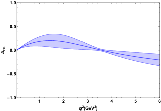
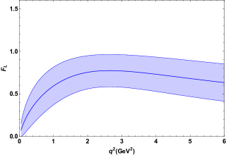
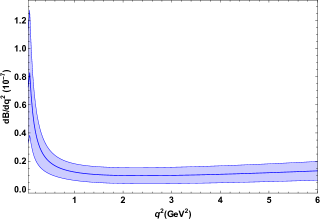
Figure 1: Differential branching fraction $d{\cal B}/dq^{2}$, forward-backward asymmetry of lepton pair, $A_{\rm FB}$, and the logitudinal polarization fraction, $F_{L}$, as function of dimuon invariant mass $q^{2}$ for $B\to K_{2}^{\ast}\mu^{+}\mu^{-}$ in the SM. The bands show estimates of uncertainties due to errors in form factors and various inputs (discussed in the text) used for the evaluation of observables.

The study of the four-fold angular distribution gives access to numerous observables that can be measured by the LHCb. Due to factorization of long and short-distance physics at large recoil Eq. (VI), one can construct observables in terms of ratios where the form factors cancel making them highly sensitive to NP. In the context of decay $B\to K^{\ast}(\to K\pi)\mu^{+}\mu^{-}$, such observables have been constructed (see, for example, Descotes-Genon:2013vna and references therein). Taking cue from $B\to K^{\ast}\ell^{+}\ell^{-}$ Matias:2012xw ; DescotesGenon:2012zf ; Descotes-Genon:2013vna , we consider following set of observables where the soft form factor cancel at leading order in $\alpha_{s}$ and $\Lambda_{\rm QCD}/m_{b}$ making them suitable probe for new physics

$$\langle P_{1}\rangle = \frac{1}{2}\frac{\displaystyle\int_{\rm bin}dq^{2}I_{3}}{\displaystyle\int_{\rm bin}dq^{2}I_{2}^{s}}\,,\quad\quad\langle P_{4}\rangle=\frac{\displaystyle\int_{\rm bin}dq^{2}I_{4}}{\sqrt{-\displaystyle\int_{\rm bin}dq^{2}I_{2}^{c}\displaystyle\int_{\rm bin}dq^{2}I_{2}^{s}}}\,,$$ (29)

$$\langle P_{2}\rangle = \frac{1}{8}\frac{\displaystyle\int_{\rm bin}dq^{2}I_{6}}{\displaystyle\int_{\rm bin}dq^{2}I_{2}^{s}}\,,\quad\quad\langle P_{5}\rangle=\frac{\displaystyle\int_{\rm bin}dq^{2}I_{5}}{2\sqrt{-\displaystyle\int_{\rm bin}dq^{2}I_{2}^{c}\displaystyle\int_{\rm bin}dq^{2}I_{2}^{s}}}\,,$$ (30)

$$\langle P_{3}\rangle = -\frac{1}{4}\frac{\displaystyle\int_{\rm bin}dq^{2}I_{9}}{\displaystyle\int_{\rm bin}dq^{2}I_{2}^{s}}\,,\quad\quad\langle P_{6}\rangle=\frac{\displaystyle\int_{\rm bin}dq^{2}I_{7}}{2\sqrt{-\displaystyle\int_{\rm bin}dq^{2}I_{2}^{c}\displaystyle\int_{\rm bin}dq^{2}I_{2}^{s}}}\,.$$ (31)

The subleading corrections to them will be estimated following the discussions in section V.

As also discussed in the Sec. I, recent LHCb results Aaij:2014ora ; Aaij:2017vbb of measurements of the ratio of $B\to K(K^{\ast})\ell^{+}\ell^{-}$ branching ratios of di-muon over di-electrons known as $R_{K,K^{\ast}}$ show significant deviation from their SM predictions $R_{K,K^{\ast}}\sim 1$ Bordone:2016gaq , which hints to violation of lepton flavor universality. Observation of the same pattern of deviation in the $K$ and $K^{\ast}$ mode is quite intriguing and has attracted a lot of attention recently (see Ref. Hiller:2017bzc for a model-independent analysis) . If NP is to blame for these, such deviations should be seen in $B\to K^{\ast}_{2}\ell^{+}\ell^{-}$ as well, and need to be studied. We define similar ratio for $B\to K^{\ast}_{2}\ell^{+}\ell^{-}$

$$R_{K^{\ast}_{2}}=\frac{\mathcal{B}(B\to K^{\ast}_{2}\mu\mu)}{\mathcal{B}(B\to K^{\ast}_{2}ee)}\,.$$ (32)

Having discussed all the observables, we are now ready to proceed with the numerical analysis of these observables in the SM and NP scenarios in the next section.

VII Numerical Analysis

In the light of the recent flavor anomalies, several groups have performed global fits of Wilson coefficients to $b\to s\ell^{+}\ell^{-}$ data to decipher the pattern of NP Descotes-Genon:2013wba ; Descotes-Genon:2015uva ; Altmannshofer:2014rta ; Hurth:2016fbr ; Altmannshofer:2015sma ; Altmannshofer:2013foa ; Beaujean:2013soa ; Hurth:2013ssa . These fits indicate that a negative contribution to the Wilson coefficient $C_{9}^{\mu}$ can alleviate the tension between theory and experimental data. There are other scenarios as well which lead to similar fits. Following Ref. Capdevila:2017bsm we consider three of them (called S1, S2, S3) having largest pull

• S1: NP in $C_{9}$ only with $C_{9}^{\mu,\rm NP}=-1.1$, for which the pull is $5.8\sigma$.

• S2: In this scenario, NP is considered in both $C_{9}$ and $C_{10}$, but they are correlated, $C_{9}^{\mu,\rm NP}=-C_{10}^{\mu,\rm NP}=-0.6$ and the pull for this scenario is $5.3\sigma$.

• S3: In this scenario, NP is considered in $C_{9}$ and $C_{9}^{\prime}$ and again correlated with best fit given by $C_{9}^{\mu,\rm NP}=-C_{9}^{\prime~{}\mu,\rm NP}=-1.01$ for which the pull is $5.4\sigma$.

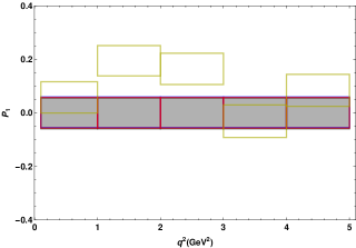
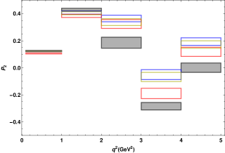
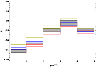
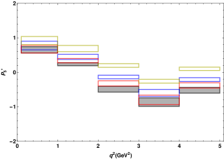
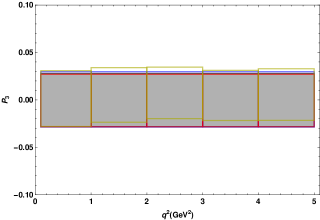
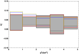
Figure 2: The clean observables $P_{i}^{(\prime)}(q^{2})~{}(i=1,2,3,4,5,6)$ in different $q^{2}$ bins in the SM (grey) and three NP scenarios S1 (blue), S2 (red) and S3 (yellow). The horizontal width of boxes corresponds to the $q^{2}$ bin size, and the vertical length gives estimate of uncertainties due to errors in form factors and other input for that particular $q^{2}$ bin.

Our main numerical results in the SM and the above three NP cases for all the angular observables considered in this work are collected in Appendix D. The binned predictions for clean observables are displayed in Fig. 2. We restrict our analysis to low dilepton invariant mass region and consider $q^{2}$ bins lying in range $0.1-6.0$ ${\rm GeV}^{2}$.

The branching fraction for $B\to K_{2}^{\ast}\mu^{+}\mu^{-}$ in the SM is $\sim{\cal O}(10^{-7})$ (see Table 1). In all three NP scenarios, we find consistently smaller central values for branching fraction compared to the SM value. This is pertaining to the fact that the global analysis of $b\to s\ell^{+}\ell^{-}$ suggests destructive NP contribution to $C_{9}^{\mu}$. For $A_{\rm FB}$ ($F_{L}$) we find slightly larger (smaller) central value in NP cases compared to the central SM value. However, as these observables ($d\Gamma/dq^{2}$, $F_{L}$ and $A_{FB}$) are at present plagued by large theoretical errors, no striking deviation from the SM value is found. On the other hand, prospects for testing NP hypothesis in $b\to s\ell^{+}\ell^{-}$ in some clean observables $P_{i}(q^{2})$ are promising.

The clean observable $P_{1}$ depends on the angular coefficients $I_{3}$ and $I_{2}$, and is of special interest due to its remarkable sensitivity to right-handed currents. The $(V-A)$ structure of the SM renders the $H_{\pm}$ helicities of the $B\to K^{\ast}_{2}\ell^{+}\ell^{-}$ suppressed, implying $|A_{\parallel}|\simeq|A_{\perp}|$. Therefore, this observable is predicted to be zero in the SM. The similar charaterstic is also shared by its $B\to K^{\ast}$ counterpart as noted in Descotes-Genon:2015uva . As shown in Fig. 2, $P_{1}$ is consistent with zero in the SM and in two scenarios S1 and S2 (which assume NP in the left-handed currents only), while a large deviations from $P_{1}\simeq 0$ is found in scenario S3 (which has nonzero value of right-handed Wilson coefficient $C_{9}^{\prime}$). The observable $P_{2}$ is similar to forward-backward asymmetry $A_{\rm FB}$, but is theoretically much cleaner. Similar to $A_{\rm FB}$, $P_{2}$ has larger values in all three NP scenarios. The zero-crossing of $P_{2}$ (same as of $A_{FB}$) lies in the [2,4] GeV² and at the leading order is given by

$$q^{2}_{0}(P_{2})\simeq-\frac{2\,C_{7}}{C_{9}-\left(C_{10}^{\prime}/C_{10}\right)C_{9}^{\prime}}m_{b}\,m_{B}.$$ (33)

In order to obtain the above relation, we have used transversity amplitudes given in Eqs. (14)-(17) and assumed the Wilson coefficients to be real. This expression is identical to the corresponding observable for $B\to K^{\ast}$ case. Note that the zero crossing $q^{2}_{0}(P_{2})$ depends on the short-distance Wilson coefficients $C_{9}^{\ell(\prime)}$ and $C_{10}^{\ell(\prime)}$, and has no dependence on the mass of lepton in final state. Consequently, in the SM it has the same value for all three decay modes $B\to K_{2}^{\ast}\ell^{+}\ell^{-}$ ($\ell=e,\mu,\tau$). Therefore the zero crossing $q^{2}_{0}(P_{2})$ turn out to be a good observable to test the hypothesis of lepton flavor universality violating (LFUV) NP.

For observables $P_{4}^{\prime}$ and $P_{5}^{\prime}$, the largest deviations from the SM value are observed in scenario S3, thereby showing good sensitivity to right-handed NP. On the other hand, observables $P_{3}$ and $P_{6}^{\prime}$ depend on $I_{9}(q^{2})$ and $I_{7}(q^{2})$ respectively. These two observables depend on imaginary part of $\rho_{\mp}^{L,R}(q^{2})$ and $\sigma_{\mp}(q^{2})$. The imaginary part of the SM Wilson coefficient $C_{9,7}^{\rm eff}$ is very tiny, and therefore the SM predictions for $P_{3}$ and $P_{6}^{\prime}$ are highly suppressed. Since, in our numerical analysis, we consider real NP Wilson coefficients, these observables remain suppressed in all three NP scenarios. Deviations in these observables, if seen in experiments, will be a sign of CP-violating NP.

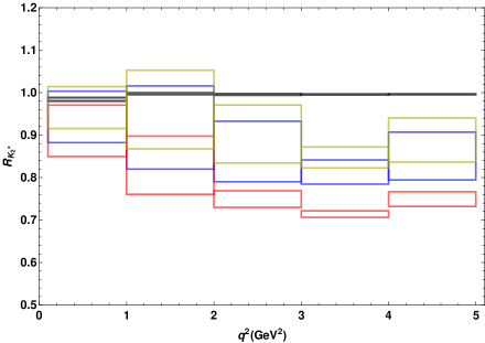
Figure 3: Binned predictions for $R_{K_{2}^{\ast}}$ in the SM (grey) and NP scenarios S1 (blue), S2 (red), and S3 (yellow).

Finally, in Fig. 3 we present our determinations of the LFUV ratio $R_{K_{2}^{\ast}}$. Similar observables for $B\to K^{(\ast)}\ell^{+}\ell^{-}$ in the SM are predicted to be $\sim 1$ Bordone:2016gaq . These LFUV ratios are exceptionally clean observables with theoretical errors being at the level of only $\sim 1\%$, making them an ideal candidate to probe NP. As mentioned earlier, $R_{K}$ and $R_{K^{\ast}}$ have been measured experimentally and both measurements are lower than the SM value, which could be interpreted as sign of NP. Therefore the measurement of $R_{K_{2}^{\ast}}$ can be important to corroborate the deviations seen in $R_{K}$ and $R_{K}^{\ast}$. In all three NP scenarios, $R_{K_{2}^{\ast}}$ is suppressed compared to the SM value. For NP case S2, the deviations from unity are largest while for NP case S3 the suppression is relatively smaller as this solution contain a mixture of left-handed and right-handed currents, and right-handed currents tend to increase the value of ratio. The bin averaged predictions for $R_{K_{2}}^{\ast}$ in the SM and NP cases are given in Appendix D.

Parameter	Value	Source
$m_{B}$	$5.279$ GeV	Tanabashi:2018oca
$m_{K_{2}^{\ast}}$	$1432.4\pm 1.3\,\text{MeV}$	Tanabashi:2018oca
$m_{b}^{\overline{\rm MS}}$	4.20 GeV	Detmold:2016pkz
$m_{b}^{\text{pole}}$	$4.7417$ GeV	Detmold:2016pkz
$m_{c}^{\text{pole}}$	$1.5953$ GeV	Detmold:2016pkz
$|V_{ts}^{*}V_{tb}|$	$0.04088\pm 0.00055$	utfit
$\alpha_{s}(\mu=4.2~{}{\rm GeV})$	0.2233	Detmold:2016pkz
$\alpha_{e}(\mu=4.2~{}{\rm GeV})$	1/133.28	Detmold:2016pkz
$Br(K_{2}^{\ast}\to K\pi)$	$(49.9\pm 1.2)\%$	Tanabashi:2018oca

Table 2: The numerical inputs used in our analysis. The values of $\alpha_{s}$, $\alpha_{e}$, and $m_{b}^{\overline{\rm MS}}$ at low scale $\mu=2.1~{}{\rm GeV}$ and high scale $\mu=8.4~{}{\rm GeV}$ are also used from Ref. Detmold:2016pkz .

	$C_{1}$	$C_{2}$	$C_{3}$	$C_{4}$	$C_{5}$	$C_{6}$	$C_{7}$	$C_{8}$	$C_{9}$	$C_{10}$
$\mu=2.1$ GeV	$-0.4965$	$1.0246$	$-0.0143$	$-0.1500$	$0.0010$	$0.0032$	$-0.3782$	$-0.2133$	$4.5692$	$-4.1602$
$\mu=4.2$ GeV	$-0.2877$	$1.0101$	$-0.0060$	$-0.0860$	$0.0004$	$0.0011$	$-0.3361$	$-0.1821$	$4.2745$	$-4.1602$
$\mu=8.4$ GeV	$-0.1488$	$1.0036$	$-0.0027$	$-0.0543$	$0.0002$	$0.0004$	$-0.3036$	$-0.1629$	$3.8698$	$-4.1602$

Table 3: Values of SM Wilson coefficients taken from Ref. Detmold:2016pkz

VIII Summary and Discussion

In this paper, we have performed an angular analysis of exclusive semileptonic decay $B\to K_{2}^{\ast}(\to K\pi)\mu^{+}\mu^{-}$. The decay, at the quark level, is governed by the $b\to s\ell^{+}\ell^{-}$ FCNC transition. About $2-3~{}\sigma$ discrepancies in $b\to s\ell^{+}\ell^{-}$ transitions have recently been observed in $B\to K(K^{\ast})\ell^{+}\ell^{-}$ decays. If these discrepancies are due to NP then similar anomalies are also expected in $B\to K_{2}^{\ast}(\to K\pi)\mu^{+}\mu^{-}$ transitions as well which make this decay worth studying.

A full angular distribution of $B\to K_{2}^{\ast}(\to K\pi)\mu^{+}\mu^{-}$ in the transversity basis, similar to $B\to K^{\ast}(\to K\pi)\mu^{+}\mu^{-}$ offers a large number of observables. We have worked in the limit of heavy quark $m_{b}\to\infty$ and large energy $E_{K_{2}^{\ast}}\to\infty$ where symmetry relations reduce the number of independent form factors from seven to two: $\xi_{\perp}(q^{2})$ and $\xi_{\parallel}(q^{2})$. Utilising these symmetry relations we have provided expressions for transversity amplitudes, and have constructed new clean angular observables. The form factor dependence for these clean observables cancel at leading order in $\alpha_{s}$ and $\Lambda_{\rm QCD}/m_{b}$. The uncertainties due to the sub-leading corrections have been included in our numerical analysis.

We have presented determinations of $B\to K_{2}^{\ast}(\to K\pi)\mu^{+}\mu^{-}$ decay rate, forward-backward asymmetry, longitudinal polarization fractions and clean observables in the SM and several NP cases . The NP scenarios are motivated by the recent global fits to the $b\to s\ell^{+}\ell^{-}$ data. We have also considered the LFU violation sensitive observable $R_{K_{2}^{\ast}}$. The $B\to K_{2}^{\ast}(\to K\pi)\mu^{+}\mu^{-}$ decay may provide new and complementary information to $B\to K^{\ast}(K)\mu^{+}\mu^{-}$ in searches of NP

Appendix A Effective Wilson coefficients for $b\to s\ell^{+}\ell^{-}$ transition

Corresponding to the $b\to s\ell^{+}\ell^{-}$ effective Hamiltonian equation (1), the one loop contributions from $\mathcal{O}_{1}-\mathcal{O}_{6}$ to the $\mathcal{O}_{7}$ and $\mathcal{O}_{9}$ are absorbed by defining the effective Wilson coefficients $C_{7}^{\rm eff}$ and $C_{9}^{\rm eff}$ Detmold:2016pkz

$$\begin{split}C_{7}^{\rm eff}(\mu)&=C_{7}-\frac{1}{3}C_{3}+\frac{4}{3}C_{4}+20C_{5}+\frac{80}{3}C_{6}-\frac{\alpha_{S}}{4\pi}\left[(C_{1}-6C_{2})F_{1,c}^{(7)}(q^{2})+C_{8}F_{8}^{(7)}(q^{2})\right],\\ C_{9}^{\rm eff}(\mu)&=C_{9}+h(q^{2},m_{c})\Big{(}\frac{4}{3}C_{1}+C_{2}+6C_{3}+60C_{5}\Big{)}\,\\ &-\frac{1}{2}h(q^{2},m_{b})\Big{(}7C_{3}+\frac{4}{3}C_{4}+76C_{5}+\frac{64}{3}C_{6}\Big{)}-\frac{1}{2}h(q^{2},0)\Big{(}C_{3}+\frac{4}{3}C_{4}+16C_{5}+\frac{64}{3}C_{6}\Big{)}\,\\ &+\frac{4}{3}C_{3}+\frac{64}{9}C_{5}+\frac{64}{27}C_{6}-\frac{\alpha_{S}}{4\pi}\left[C_{1}F_{1,c}^{(9)}(q^{2})+C_{2}F_{2,c}^{(9)}(q^{2})+C_{8}F_{8}^{(9)}(q^{2})\right].\end{split}$$ (34)

The value of the SM Wilson coefficients $C_{i}$ $(i=1,2,..10)$ are given in Table 3. The functions $h(q^{2},m_{q})$ and $F_{8}^{(7,9)}(q^{2})$ can be found in Ref. Beneke:2001at , and the functions $F_{1,2}^{(7,9)}(q^{2})$ are taken from Ref. Asatryan:2001zw . The values of masses of charm and bottom quark in these expressions are defined in pole mass scheme and are given in Table 2.

Appendix B $K_{2}^{\ast}$ polarization tensors

The tensor meson $K_{2}^{\ast}$ is described in terms of spin-2 polarization tensor $\epsilon^{\mu\nu}(n)$, where the helicity $n$ can be $\pm 2,\pm 1$ and 0. The polarization tensor satisfy $\epsilon^{\mu\nu}k^{\nu}=0$. For the $K_{2}^{\ast}$ which has four momentum $(k_{0},0,0,\vec{k})$, the polarization tensor $\epsilon^{\mu\nu}(h)$ can be constructed in terms of following polarization tensors Berger:2000wt

$$\epsilon_{\mu}(0)=\frac{1}{m_{K_{2}^{\ast}}}(|\vec{k}|,0,0,k_{0})\,,\quad\epsilon_{\mu}(\pm)=\frac{1}{\sqrt{2}}(0,\mp 1,-i,0)\,,$$

in the following way

$$\epsilon_{\mu\nu}(\pm 2)=\epsilon_{\mu}(\pm 1)\epsilon_{\nu}(\pm 1)\,,\quad\epsilon_{\mu\nu}(\pm 1)=\frac{1}{\sqrt{2}}\Big{[}\epsilon_{\nu}(\pm)\epsilon_{\nu}(0)+\epsilon_{\nu}(\pm)\epsilon_{\mu}(0)\Big{]}\,,$$

$$\epsilon_{\mu\nu}(0)=\frac{1}{\sqrt{6}}\Big{[}\epsilon_{\mu}(+)\epsilon_{\nu}(-)+\epsilon_{\nu}(+)\epsilon_{\mu}(-)\Big{]}+\sqrt{\frac{2}{3}}\epsilon_{\mu}(0)\epsilon_{\nu}(0)\,.$$

In the decay under consideration, since there are two leptons in the final state the $n=\pm 2$ helicity states of the $K_{2}^{\ast}$ is not realized. It is therefore convenient to introduce a new polarization vector Wang:2010ni

$$\epsilon_{T\mu}(h)=\frac{\epsilon_{\mu\nu}p^{\nu}}{m_{B}}\,,$$

where $p$ is the four momentum of $B$ meson. The explicit expressions of polarization vectors are

$$\epsilon_{T\mu}(\pm 1) = \frac{1}{m_{B}}\frac{1}{\sqrt{2}}\epsilon(0).p\,\epsilon_{\mu}(\pm)=\frac{\sqrt{\lambda}}{\sqrt{8}m_{B}m_{K_{2}}^{\ast}}\epsilon_{\mu}(\pm)\,,$$ (35)

$$\epsilon_{T\mu}(0) = \frac{1}{m_{B}}\sqrt{\frac{2}{3}}\epsilon(0).p\,\epsilon_{\mu}(0)=\frac{\sqrt{\lambda}}{\sqrt{6}m_{B}m_{K_{2}}^{\ast}}\epsilon_{\mu}(0)\,,$$ (36)

where $\lambda=m_{B}^{4}+m_{K_{2}^{\ast}}^{4}+q^{4}-2(m_{B}^{2}m_{K_{2}^{\ast}}^{2}+m_{B}^{2}q^{2}+m_{K_{2}^{\ast}}^{2}q^{2})$.

Appendix C Angular Coefficients $I_{i}(q^{2})$

Here we summarize the expressions of the angular coefficients appearing in the differential decay rate eq. (20) in terms of transversity amplitudes Li:2010ra

$$I_{1}^{c} = (|A_{0L}|^{2}+|A_{0R}|^{2})+8\frac{m_{\ell}^{2}}{q^{2}}{\rm Re}[A_{0L}A^{*}_{0R}]+4\frac{m_{\ell}^{2}}{q^{2}}|A_{t}|^{2},$$

$$I_{1}^{s} = \frac{3}{4}\left(1-\frac{4m_{\ell}^{2}}{3q^{2}}\right)[|A_{\perp L}|^{2}+|A_{||L}|^{2}+|A_{\perp R}|^{2}+|A_{||R}|^{2}]+\frac{4m_{\ell}^{2}}{q^{2}}{\rm Re}[A_{\perp L}A_{\perp R}^{*}+A_{||L}A_{||R}^{*}],$$

$$I_{2}^{c} = -\beta_{\ell}^{2}(|A_{0L}|^{2}+|A_{0R}|^{2})\,,\quad I_{2}^{s}=\frac{1}{4}\beta_{l}^{2}(|A_{\perp L}|^{2}+|A_{||L}|^{2}+|A_{\perp R}|^{2}+|A_{||R}|^{2}),$$

$$I_{3} = \frac{1}{2}\beta_{l}^{2}(|A_{\perp L}|^{2}-|A_{||L}|^{2}+|A_{\perp R}|^{2}-|A_{||R}|^{2})\,$$ (37)

$$I_{4} = \frac{1}{\sqrt{2}}\beta_{\ell}^{2}[{\rm Re}(A_{0L}A_{||L}^{*})+{\rm Re}(A_{0R}A_{||R}^{*}]\,,\quad I_{5}=\sqrt{2}\beta_{l}[{\rm Re}(A_{0L}A_{\perp L}^{*})-{\rm Re}(A_{0R}A_{\perp R}^{*})],$$

$$I_{6} = 2\beta_{\ell}[{\rm Re}(A_{||L}A^{*}_{\perp L})-{\rm Re}(A_{||R}A^{*}_{\perp R})]\,,\quad I_{7}=\sqrt{2}\beta_{\ell}[{\rm Im}(A_{0L}A^{*}_{||L})-{\rm Im}(A_{0R}A^{*}_{||R})],$$

$$I_{8} = \frac{1}{\sqrt{2}}\beta_{\ell}^{2}[{\rm Im}(A_{0L}A^{*}_{\perp L})+{\rm Im}(A_{0R}A^{*}_{\perp R})]\,,\quad I_{9}=\beta_{\ell}^{2}[{\rm Im}(A_{||L}A^{*}_{\perp L})+{\rm Im}(A_{||R}A^{*}_{\perp R})],$$

where $\beta_{\ell}=\sqrt{1-\frac{4m^{2}_{\ell}}{q^{2}}}$.

Appendix D

D.1 Prediction of observables in the SM

Bin	$P_{1}$	$P_{2}$	$P_{3}$
$[0.1,1]$	$0.001\pm 0.059$	$0.125\pm 0.004$	$0.0\pm 0.028$
$[1,2]$	$0.001\pm 0.059$	$0.431\pm 0.009$	$0.0\pm 0.028$
$[2,4]$	$0.001\pm 0.059$	$0.186\pm 0.041$	$0.0\pm 0.028$
$[4,6]$	$0.001\pm 0.059$	$-0.284\pm 0.028$	$0.0\pm 0.028$
$[1,6]$	$0.001\pm 0.059$	$0.001\pm 0.035$	$0.0\pm 0.028$
Bin	$P_{4}^{\prime}$	$P_{5}^{\prime}$	$P_{6}^{\prime}$
$[0.1,1]$	$-0.560\pm 0.084$	$0.652\pm 0.093$	$0.035\pm 0.042$
$[1,2]$	$-0.178\pm 0.034$	$0.235\pm 0.0.045$	$0.043\pm 0.023$
$[2,4]$	$0.527\pm 0.086$	$-0.489\pm 0.083$	$0.040\pm 0.034$
$[4,6]$	$0.878\pm 0.132$	$-0.864\pm 0.124$	$0.026\pm 0.053$
$[1,6]$	$0.550\pm 0.087$	$-0.520\pm 0.083$	$0.034\pm 0.034$
Bin	$BR~{}(10^{-7})$	$A_{FB}$	$F_{L}$
$[0.1,1]$	$0.205\pm 0.093$	$0.094\pm 0.029$	$0.346\pm 0.198$
$[1,2]$	$0.104\pm 0.055$	$0.202\pm 0.133$	$0.686\pm 0.208$
$[2,4]$	$0.196\pm 0.119$	$0.070\pm 0.059$	$0.760\pm 0.191$
$[4,6]$	$0.232\pm 0.122$	$-0.141\pm 0.094$	$0.679\pm 0.210$
$[1,6]$	$0.532\pm 0.289$	$0.0\pm 0.019$	$0.709\pm 0.204$

D.2 Prediction of observables in the NP scenario S1 ($C_{9}^{\mu,{\rm NP}}=-1.1$)

Bin	$P_{1}$	$P_{2}$	$P_{3}$
$[0.1,1]$	$0.003\pm 0.057$	$0.123\pm 0.004$	$0.0\pm 0.029$
$[1,2]$	$0.003\pm 0.057$	$0.408\pm 0.011$	$0.0\pm 0.029$
$[2,4]$	$0.003\pm 0.057$	$0.365\pm 0.024$	$0.0\pm 0.029$
$[4,6]$	$0.003\pm 0.057$	$-0.050\pm 0.037$	$0.0\pm 0.029$
$[1,6]$	$0.003\pm 0.057$	$0.194\pm 0.028$	$0.0\pm 0.029$
Bin	$P_{4}^{\prime}$	$P_{5}^{\prime}$	$P_{6}^{\prime}$
$[0.1,1]$	$-0.434\pm 0.041$	$0.777\pm 0.124$	$0.041\pm 0.047$
$[1,2]$	$-0.093\pm 0.016$	$0.448\pm 0.076$	$0.048\pm 0.031$
$[2,4]$	$0.474\pm 0.053$	$-0.136\pm 0.052$	$0.041\pm 0.018$
$[4,6]$	$0.837\pm 0.081$	$-0.597\pm 0.102$	$0.027\pm 0.037$
$[1,6]$	$0.509\pm 0.054$	$-0.210\pm 0.056$	$0.036\pm 0.019$
Bin	$BR~{}(10^{-7})$	$A_{FB}$	$F_{L}$
$[0.1,1]$	$0.201\pm 0.094$	$0.100\pm 0.026$	$0.288\pm 0.188$
$[1,2]$	$0.093\pm 0.046$	$0.240\pm 0.130$	$0.594\pm 0.222$
$[2,4]$	$0.165\pm 0.090$	$0.170\pm 0.115$	$0.691\pm 0.210$
$[4,6]$	$0.188\pm 0.097$	$-0.027\pm 0.028$	$0.644\pm 0.218$
$[1,6]$	$0.446\pm 0.232$	$0.102\pm 0.065$	$0.650\pm 0.217$

D.3 Prediction of observables in the NP scenario S2 ($C_{9}^{\mu,{\rm NP}}=-C_{10}^{\mu,{\rm NP}}=-0.6$)

Bin	$P_{1}$	$P_{2}$	$P_{3}$
$[0.1,1]$	$0.0\pm 0.057$	$0.107\pm 0.004$	$0.0\pm 0.028$
$[1,2]$	$0.0\pm 0.057$	$0.384\pm 0.012$	$0.0\pm 0.028$
$[2,4]$	$0.0\pm 0.057$	$0.325\pm 0.033$	$0.0\pm 0.028$
$[4,6]$	$0.0\pm 0.057$	$-0.189\pm 0.038$	$0.0\pm 0.028$
$[1,6]$	$0.0\pm 0.057$	$0.118\pm 0.034$	$0.0\pm 0.028$
Bin	$P_{4}^{\prime}$	$P_{5}^{\prime}$	$P_{6}^{\prime}$
$[0.1,1]$	$-0.577\pm 0.082$	$0.673\pm 0.118$	$0.037\pm 0.042$
$[1,2]$	$-0.275\pm 0.042$	$0.339\pm 0.064$	$0.043\pm 0.027$
$[2,4]$	$0.374\pm 0.065$	$-0.321\pm 0.139$	$0.043\pm 0.026$
$[4,6]$	$0.826\pm 0.118$	$-0.899\pm 0.183$	$0.028\pm 0.049$
$[1,6]$	$0.423\pm 0.068$	$-0.582\pm 0.131$	$0.037\pm 0.027$
Bin	$BR~{}(10^{-7})$	$A_{FB}$	$F_{L}$
$[0.1,1]$	$0.189\pm 0.091$	$0.087\pm 0.023$	$0.284\pm 0.186$
$[1,2]$	$0.083\pm 0.042$	$0.213\pm 0.119$	$0.616\pm 0.219$
$[2,4]$	$0.144\pm 0.084$	$0.128\pm 0.097$	$0.738\pm 0.198$
$[4,6]$	$0.165\pm 0.091$	$-0.090\pm 0.063$	$0.685\pm 0.209$
$[1,6]$	$0.393\pm 0.217$	$0.055\pm 0.041$	$0.688\pm 0.209$

D.4 Prediction of observables in the NP scenario S3 ($C_{9}^{\mu,{\rm NP}}=-C_{9}^{\prime\mu,{\rm NP}}=-1.01$)

Bin	$P_{1}$	$P_{2}$	$P_{3}$
$[0.1,1]$	$0.058\pm 0.058$	$0.123\pm 0.004$	$0.001\pm 0.029$
$[1,2]$	$0.195\pm 0.057$	$0.404\pm 0.011$	$0.005\pm 0.029$
$[2,4]$	$0.165\pm 0.058$	$0.338\pm 0.026$	$0.007\pm 0.027$
$[4,6]$	$-0.031\pm 0.061$	$-0.068\pm 0.034$	$0.005\pm 0.026$
$[1,6]$	$0.084\pm 0.060$	$0.172\pm 0.028$	$0.006\pm 0.027$
Bin	$P_{4}^{\prime}$	$P_{5}^{\prime}$	$P_{6}^{\prime}$
$[0.1,1]$	$-0.265\pm 0.032$	$0.921\pm 0.119$	$0.044\pm 0.051$
$[1,2]$	$0.124\pm 0.022$	$0.689\pm 0.091$	$0.048\pm 0.033$
$[2,4]$	$0.694\pm 0.087$	$0.198\pm 0.053$	$0.044\pm 0.021$
$[4,6]$	$0.993\pm 0.119$	$-0.258\pm 0.056$	$0.030\pm 0.040$
$[1,6]$	$0.704\pm 0.087$	$0.103\pm 0.048$	$0.039\pm 0.022$
Bin	$BR~{}(10^{-7})$	$A_{FB}$	$F_{L}$
$[0.1,1]$	$0.189\pm 0.093$	$0.105\pm 0.025$	$0.261\pm 0.181$
$[1,2]$	$0.083\pm 0.042$	$0.262\pm 0.130$	$0.559\pm 0.226$
$[2,4]$	$0.146\pm 0.080$	$0.179\pm 0.112$	$0.653\pm 0.218$
$[4,6]$	$0.169\pm 0.088$	$-0.041\pm 0.033$	$0.599\pm 0.225$
$[1,6]$	$0.398\pm 0.208$	$0.102\pm 0.061$	$0.610\pm 0.223$

D.5 Prediction of $R_{K_{2}^{\ast}}$

Bin	SM	S1	S2	S3
$[0.1,1]$	$0.986\pm 0.005$	$0.943\pm 0.061$	$0.910\pm 0.060$	$0.96\pm 0.049$
$[1,2]$	$0.998\pm 0.003$	$0.918\pm 0.098$	$0.829\pm 0.068$	$0.960\pm 0.092$
$[2,4]$	$0.996\pm 0.002$	$0.861\pm 0.071$	$0.749\pm 0.020$	$0.903\pm 0.068$
$[4,6]$	$0.996\pm 0.002$	$0.813\pm 0.028$	$0.714\pm 0.008$	$0.847\pm 0.025$
$[1,6]$	$0.996\pm 0.002$	$0.851\pm 0.056$	$0.749\pm 0.017$	$0.888\pm 0.052$

References

• (1) LHCb, R.ย Aaij et al., โ€œTest of lepton universality using $B^{+}\rightarrow K^{+}\ell^{+}\ell^{-}$ decays,โ€ Phys. Rev. Lett. 113 (2014) 151601, arXiv:1406.6482.
• (2) LHCb, R.ย Aaij et al., โ€œTest of lepton universality with $B^{0}\rightarrow K^{*0}\ell^{+}\ell^{-}$ decays,โ€ JHEP 08 (2017) 055, arXiv:1705.05802.
• (3) S.ย Descotes-Genon, J.ย Matias, and J.ย Virto, โ€œUnderstanding the $B\to K^{*}\mu^{+}\mu^{-}$ Anomaly,โ€ Phys. Rev. D88 (2013) 074002, arXiv:1307.5683.
• (4) LHCb, R.ย Aaij et al., โ€œMeasurement of Form-Factor-Independent Observables in the Decay $B^{0}\to K^{*0}\mu^{+}\mu^{-}$,โ€ Phys. Rev. Lett. 111 (2013) 191801, arXiv:1308.1707.
• (5) LHCb, R.ย Aaij et al., โ€œAngular analysis of the $B^{0}\to K^{*0}\mu^{+}\mu^{-}$ decay using 3 fb-1 of integrated luminosity,โ€ JHEP 02 (2016) 104, arXiv:1512.04442.
• (6) Belle, A.ย Abdesselam et al., โ€œAngular analysis of $B^{0}\to K^{\ast}(892)^{0}\ell^{+}\ell^{-}$,โ€ in Proceedings, LHCSki 2016 - A First Discussion of 13 TeV Results: Obergurgl, Austria, April 10-15, 2016. 2016. arXiv:1604.04042.
• (7) Belle, S.ย Wehle et al., โ€œLepton-Flavor-Dependent Angular Analysis of $B\to K^{\ast}\ell^{+}\ell^{-}$,โ€ Phys. Rev. Lett. 118 (2017) no.ย 11, 111801, arXiv:1612.05014.
• (8) ATLAS, T.ย A. collaboration, โ€œAngular analysis of $B^{0}_{d}\to K^{*}\mu^{+}\mu^{-}$ decays in $pp$ collisions at s=8๐‘ 8\sqrt{s}=8 TeV with the ATLAS detector,โ€.
• (9) CMS, C.ย Collaboration, โ€œMeasurement of the $P_{1}$ and $P_{5}^{\prime}$ angular parameters of the decay $\mathrm{B}^{0}\to\mathrm{K}^{*0}\mu^{+}\mu^{-}$ in proton-proton collisions at s=8โ€‹TeV๐‘ 8TeV\sqrt{s}=8~{}\mathrm{TeV},โ€.
• (10) LHCb, R.ย Aaij et al., โ€œAngular analysis and differential branching fraction of the decay Bs0โ†’ฯ•โ€‹ฮผ+โ€‹ฮผโˆ’โ†’subscriptsuperscript๐ต0๐‘ italic-ฯ•superscript๐œ‡superscript๐œ‡B^{0}_{s}\to\phi\mu^{+}\mu^{-},โ€ JHEP 09 (2015) 179, arXiv:1506.08777.
• (11) S.ย Descotes-Genon, L.ย Hofer, J.ย Matias, and J.ย Virto, โ€œGlobal analysis of bโ†’sโ€‹โ„“โ€‹โ„“โ†’๐‘๐‘ โ„“โ„“b\to s\ell\ell anomalies,โ€ JHEP 06 (2016) 092, arXiv:1510.04239.
• (12) W.ย Altmannshofer and D.ย M. Straub, โ€œNew physics in bโ†’sโ†’๐‘๐‘ b\rightarrow s transitions after LHC run 1,โ€ Eur. Phys. J. C75 (2015) no.ย 8, 382, arXiv:1411.3161.
• (13) T.ย Hurth, F.ย Mahmoudi, and S.ย Neshatpour, โ€œOn the anomalies in the latest LHCb data,โ€ Nucl. Phys. B909 (2016) 737โ€“777, arXiv:1603.00865.
• (14) W.ย Altmannshofer and D.ย M. Straub, โ€œImplications of bโ†’sโ†’๐‘๐‘ b\to s measurements,โ€ in Proceedings, 50th Rencontres de Moriond Electroweak Interactions and Unified Theories: La Thuile, Italy, March 14-21, 2015, pp.ย 333โ€“338. 2015. arXiv:1503.06199.
• (15) W.ย Altmannshofer and D.ย M. Straub, โ€œNew Physics in $B\to K^{*}\mu\mu$?,โ€ Eur. Phys. J. C73 (2013) 2646, arXiv:1308.1501.
• (16) F.ย Beaujean, C.ย Bobeth, and D.ย van Dyk, โ€œComprehensive Bayesian analysis of rare (semi)leptonic and radiative $B$ decays,โ€ Eur. Phys. J. C74 (2014) 2897, arXiv:1310.2478. [Erratum: Eur. Phys. J.C74,3179(2014)].
• (17) T.ย Hurth and F.ย Mahmoudi, โ€œOn the LHCb anomaly in B $\to K^{*}\ell^{+}\ell^{-}$,โ€ JHEP 04 (2014) 097, arXiv:1312.5267.
• (18) BaBar, B.ย Aubert et al., โ€œMeasurement of the $B^{0}\to K^{*}_{2}(1430)^{0}\gamma$ and $B^{+}\to K^{*}_{2}(1430)^{+}\gamma$ branching fractions,โ€ Phys. Rev. D70 (2004) 091105, arXiv:hep-ex/0409035.
• (19) Belle, S.ย Nishida et al., โ€œRadiative B meson decays into K pi gamma and K pi pi gamma final states,โ€ Phys. Rev. Lett. 89 (2002) 231801, arXiv:hep-ex/0205025.
• (20) S.ย Raiย Choudhury, A.ย S. Cornell, G.ย C. Joshi, and B.ย H.ย J. McKellar, โ€œAnalysis of the B โ€”ยฟ K*(2)(โ€”ยฟ K pi) l+ l- decay,โ€ Phys. Rev. D74 (2006) 054031, arXiv:hep-ph/0607289.
• (21) S.ย R. Choudhury, A.ย S. Cornell, and N.ย Gaur, โ€œAnalysis of the anti-B โ€”ยฟ anti-K(2)(1430) l+ l- decay,โ€ Phys. Rev. D81 (2010) 094018, arXiv:0911.4783.
• (22) H.ย Hatanaka and K.-C. Yang, โ€œRadiative and Semileptonic B Decays Involving the Tensor Meson K(2)*(1430) in the Standard Model and Beyond,โ€ Phys. Rev. D79 (2009) 114008, arXiv:0903.1917.
• (23) H.ย Hatanaka and K.-C. Yang, โ€œRadiative and Semileptonic B Decays Involving Higher K-Resonances in the Final States,โ€ Eur. Phys. J. C67 (2010) 149โ€“162, arXiv:0907.1496.
• (24) W.ย Wang, โ€œB to tensor meson form factors in the perturbative QCD approach,โ€ Phys. Rev. D83 (2011) 014008, arXiv:1008.5326.
• (25) H.-Y. Cheng, Y.ย Koike, and K.-C. Yang, โ€œTwo-parton Light-cone Distribution Amplitudes of Tensor Mesons,โ€ Phys. Rev. D82 (2010) 054019, arXiv:1007.3541.
• (26) Z.-G. Wang, โ€œAnalysis of the $B\to K^{*}_{2}(1430),a_{2}(1320),f_{2}(1270)$ form-factors with light-cone QCD sum rules,โ€ Mod. Phys. Lett. A26 (2011) 2761โ€“2782, arXiv:1011.3200.
• (27) K.-C. Yang, โ€œB to Light Tensor Meson Form Factors Derived from Light-Cone Sum Rules,โ€ Phys. Lett. B695 (2011) 444โ€“448, arXiv:1010.2944.
• (28) I.ย Ahmed, M.ย J. Aslam, M.ย Junaid, and S.ย Shafaq, โ€œModel independent analysis of B โ€”ยฟ K*(2) (1430) mu+ mu- decay,โ€ JHEP 02 (2012) 045.
• (29) M.ย Junaid, M.ย J. Aslam, and I.ย Ahmed, โ€œComplementarity of Semileptonic $B$ to $K_{2}^{*}(1430)$ and $K^{*}(892)$ Decays in the Standard Model with Fourth Generation,โ€ Int. J. Mod. Phys. A27 (2012) 1250149, arXiv:1103.3934.
• (30) R.-H. Li, C.-D. Lu, and W.ย Wang, โ€œBranching ratios, forward-backward asymmetries and angular distributions of $B\to K_{2}^{*}l^{+}l^{-}$ in the standard model and new physics scenarios,โ€ Phys. Rev. D83 (2011) 034034, arXiv:1012.2129.
• (31) C.-D. Lu and W.ย Wang, โ€œAnalysis of $B\to K^{*}_{J}(\to K\pi)\mu^{+}\mu^{-}$ in the higher kaon resonance region,โ€ Phys. Rev. D85 (2012) 034014, arXiv:1111.1513.
• (32) T.ย M. Aliev and M.ย Savci, โ€œBโ†’K2โ€‹โ„“+โ€‹โ„“โˆ’โ†’๐ตsubscript๐พ2superscriptโ„“superscriptโ„“B\to K_{2}\ell^{+}\ell^{-} decay beyond the Standard Model,โ€ Phys. Rev. D85 (2012) 015007, arXiv:1109.2738.
• (33) W.ย Detmold and S.ย Meinel, โ€œฮ›bโ†’ฮ›โ€‹โ„“+โ€‹โ„“โˆ’โ†’subscriptฮ›๐‘ฮ›superscriptโ„“superscriptโ„“\Lambda_{b}\to\Lambda\ell^{+}\ell^{-} form factors, differential branching fraction, and angular observables from lattice QCD with relativistic $b$ quarks,โ€ Phys. Rev. D93 (2016) no.ย 7, 074501, arXiv:1602.01399.
• (34) M.ย Beneke, T.ย Feldmann, and D.ย Seidel, โ€œSystematic approach to exclusive $B\to Vl^{+}l^{-}$, $V\gamma$ decays,โ€ Nucl. Phys. B612 (2001) 25โ€“58, arXiv:hep-ph/0106067.
• (35) M.ย Beneke, T.ย Feldmann, and D.ย Seidel, โ€œExclusive radiative and electroweak $b\to d$ and bโ†’sโ†’๐‘๐‘ b\to s penguin decays at NLO,โ€ Eur. Phys. J. C41 (2005) 173โ€“188, arXiv:hep-ph/0412400.
• (36) A.ย Paul and D.ย M. Straub, โ€œConstraints on new physics from radiative $B$ decays,โ€ JHEP 04 (2017) 027, arXiv:1608.02556.
• (37) E.ย R. Berger, A.ย Donnachie, H.ย G. Dosch, and O.ย Nachtmann, โ€œObserving the odderon: Tensor meson photoproduction,โ€ Eur. Phys. J. C14 (2000) 673โ€“682, arXiv:hep-ph/0001270.
• (38) M.ย J. Dugan and B.ย Grinstein, โ€œQCD basis for factorization in decays of heavy mesons,โ€ Phys. Lett. B255 (1991) 583โ€“588.
• (39) J.ย Charles, A.ย Leย Yaouanc, L.ย Oliver, O.ย Pene, and J.ย C. Raynal, โ€œHeavy to light form-factors in the heavy mass to large energy limit of QCD,โ€ Phys. Rev. D60 (1999) 014001, arXiv:hep-ph/9812358.
• (40) M.ย Wirbel, B.ย Stech, and M.ย Bauer, โ€œExclusive Semileptonic Decays of Heavy Mesons,โ€ Z. Phys. C29 (1985) 637.
• (41) U.ย Egede, T.ย Hurth, J.ย Matias, M.ย Ramon, and W.ย Reece, โ€œNew physics reach of the decay mode $\bar{B}\to\bar{K}^{*0}\ell^{+}\ell^{-}$,โ€ JHEP 10 (2010) 056, arXiv:1005.0571.
• (42) S.ย Descotes-Genon, T.ย Hurth, J.ย Matias, and J.ย Virto, โ€œOptimizing the basis of $B\to K^{*}ll$ observables in the full kinematic range,โ€ JHEP 05 (2013) 137, arXiv:1303.5794.
• (43) J.ย Matias, F.ย Mescia, M.ย Ramon, and J.ย Virto, โ€œComplete Anatomy of $\bar{B}_{d}->\bar{K}^{*0}(->K\pi)l^{+}l^{-}$ and its angular distribution,โ€ JHEP 04 (2012) 104, arXiv:1202.4266.
• (44) S.ย Descotes-Genon, J.ย Matias, M.ย Ramon, and J.ย Virto, โ€œImplications from clean observables for the binned analysis of $B->K*\mu^{+}\mu^{-}$ at large recoil,โ€ JHEP 01 (2013) 048, arXiv:1207.2753.
• (45) M.ย Bordone, G.ย Isidori, and A.ย Pattori, โ€œOn the Standard Model predictions for $R_{K}$ and $R_{K^{*}}$,โ€ Eur. Phys. J. C76 (2016) no.ย 8, 440, arXiv:1605.07633.
• (46) G.ย Hiller and I.ย Nisandzic, โ€œRKsubscript๐‘…๐พR_{K} and $R_{K^{\ast}}$ beyond the standard model,โ€ Phys. Rev. D96 (2017) no.ย 3, 035003, arXiv:1704.05444.
• (47) B.ย Capdevila, A.ย Crivellin, S.ย Descotes-Genon, J.ย Matias, and J.ย Virto, โ€œPatterns of New Physics in bโ†’sโ€‹โ„“+โ€‹โ„“โˆ’โ†’๐‘๐‘ superscriptโ„“superscriptโ„“b\to s\ell^{+}\ell^{-} transitions in the light of recent data,โ€ JHEP 01 (2018) 093, arXiv:1704.05340.
• (48) Particle Data Group, M.ย Tanabashi et al., โ€œReview of Particle Physics,โ€ Phys. Rev. D98 (2018) no.ย 3, 030001.
• (49) UTfit. http://www.utfit.org/UTfit/ResultsSummer2014PostMoriondSM.
• (50) H.ย H. Asatryan, H.ย M. Asatrian, C.ย Greub, and M.ย Walker, โ€œCalculation of two loop virtual corrections to bโ†’sโ€‹l+โ€‹lโˆ’โ†’๐‘๐‘ superscript๐‘™superscript๐‘™b\to sl^{+}l^{-} in the standard model,โ€ Phys. Rev. D65 (2002) 074004, arXiv:hep-ph/0109140.