Regularized Binary Network Training

Abstract

There is a significant performance gap between Binary Neural Networks (BNNs) and floating point Deep Neural Networks (DNNs). We propose to improve the binary training method, by introducing a new regularization function that encourages training weights around binary values. In addition, we add trainable scaling factors to our regularization functions. Additionally, an improved approximation of the derivative of the $\operatorname{sign}$ activation function in the backward computation. These modifications are based on linear operations that are easily implementable into the binary training framework. Experimental results on ImageNet shows our method outperforms the traditional BNN method and XNOR-net.

1 Introduction

DNNs are heavy to compute on low resource devices. There have been several approaches developed to overcome this issue, such as network pruning (LeCun et al., 1990), architecture design (Sandler et al., 2018), and quantization (Courbariaux et al., 2015; Han et al., 2015). In particular, weight compression using quantization can achieve very large savings in memory, where binary (1-bit), and ternary (2-bit) approaches have been shown to obtain competitive accuracy as compared to their full precision counterpart (Hubara et al., 2018; Zhu et al., 2016; Tang et al., 2017).

Our contribution consists of three ideas that can be easily implemented in the binary training framework presented by Hubara et al. (2018) to improve convergence and generalization of binary neural networks. First, we improve the straight-through estimator introduced in Hubara et al. (2018), Second, we propose a new regularization function that encourage training weights around binary values. Third, a scaling factor is introduced in the regularization function as well as network building blocks to mitigate accuracy drop due to hard binarization.

Training a binary neural network faces two major challenges: quantizing the weights, and the activation functions. As both weights and activations are binary, the traditional continuous optimization methods such as SGD cannot be directly applied. Instead, a continuous approximation is used for the $\operatorname{sign}$ activation during the backward pass.

The general training framework is depicted in Figure 1. In Hubara et al. (2018), the weights are quantized by using the $\operatorname{sign}$ function which is $+1$ if $w>0$ and $-1$ otherwise.

Binary training use heuristics to approximating the gradient of a neuron,

$$\frac{dL(w)}{dw}\approx\frac{dL}{dw}\bigg{\rvert}_{w=w^{b}}\bm{1}_{\{|w|\leq 1\}}$$ (1)

where $L$ is the loss function, $\bm{1}(.)$ is the indicator function and $w^{b}$ is the binarized weight. The gradients in the backward pass are then applied to weights that are within $[-1,+1]$. The training process is summarized in Figure 1. As weights undergo gradient updates, they are eventually pushed out of the center region and instead make two modes, one at $-1$ and another at $+1$.

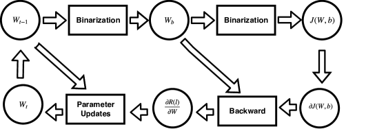
Figure 1: Binary training where arrows indicate operands flowing into operations or blocks.

2 Gradient Approximation

Our first modification is on closing the discrepancy between the forward pass and backward pass. Originally, the $\operatorname{sign}$ function derivative is approximated using the $\mathrm{htanh}(x)$ activation derivative as shown in Figure 2. Instead, we modify the Swish-like activation (Ramachandran et al., 2017; Elfwing et al., 2018; Hendrycks and Gimpel, 2016), which has been shown to outperform other activation functions on various tasks. The modifications are performed by taking its derivative and centering it around 0. Let $\mathrm{SS}_{\beta}(x)=2\sigma(\beta x)\left[1+\beta x\{1-\sigma(\beta x)\}\right]-1,$ where $\sigma(z)$ is the sigmoid function and the scale $\beta>0$ controls how fast the activation function asymptotes to $-1$ and $+1$. The $\beta$ parameter can be learned by the network or be hand-tuned as a hyperparameter. As opposed to the Swish function, where it is unbounded on the right side, the modification makes it bounded, a more valid approximator of the $\operatorname{sign}$ function so we call this activation SignSwish or SSwish, see Figure 2.

Figure 2: Forward and backward approximations. The forward and backward functions of SignSwish $SS_{\beta}(x)$ for $\beta=1$. and $\beta=5$.

Hubara et al. (2018) noted that the Straight-through Estimator (STE) fails to learn weights near the borders of $-1$ and $+1$. As depicted in Figure 2, our proposed SignSwish activation alleviates this issue, as it remains differentiable near $-1$ and $+1$ allowing weights to change signs during training if necessary.

Note that the derivative $\frac{d\mathrm{SS}_{\beta}(x)}{dx}$ is zero at two points, controlled by $\beta$. Indeed, it is simple to show that the derivative is zero for $x\approx\pm 2.4/\beta$. By adjusting this parameter, it is possible to adjust the location at which the gradients start saturating, in contrast with the STE estimators where it is fixed.

3 Regularization function

In general, a regularization term is added to a model to prevent over-fitting and to obtain robust generalization. The two most commonly used regularization terms are $L_{1}$ and $L_{2}$ norms. If one were to embed these regularization functions in binary training, it would encourage the weights to be near zero, though this does not align with the objective of a binary network. A regularization function for binary networks should vanish upon the quantized values. Following this intuition, we define a function that encourages the weights around $-1$ and $+1$. The Manhattan $R_{1}(.)$ and Euclidean $R_{2}(.)$ regularization functions are defined as

$$R_{1}(w)=|\alpha-|w||,\quad R_{2}(w)=(\alpha-|w|)^{2},$$ (2)

where $\alpha\in\rm I\!R^{+}$. In Figure 3, we depict the different regularization terms to help with intuition.

Figure 3: Regularization functions for $\alpha=0.5$ (solid line) and $\alpha=1$ (dashed line).

These regularization functions encode a quantization structure, when added to the overall loss function of the network encouraging weights to binary values. The difference between the two is in the rate at which weights are penalized when far from the binary objective, $L_{1}$ linearly penalizes the weights and is non-smooth compared to the $L_{2}$ version where weights are penalized quadritically. We further relax the hard thresholding of binary values $\{-1,1\}$ by introducing scales $\alpha$ in the regularization function. This results in a symmetric regularization function with two minimums, one at $-\alpha$ and another at $+\alpha$. The scales are then added to the networks and multiplied into the weights after the binarization operation. As these scales are introduced in the regularization function and are embedded into the layers of the network they can be learned using back-propagation. This is in contrast with the scales introduced in Rastegari et al. (2016), where they compute the scales dynamically during training using the statistics of the weights after every training batch. As depicted in Figure 3, in the case of $\alpha=1$, the weights are penalized at varying degrees upon moving away from the objective quantization values, in this case, $\{-1,+1\}$.

4 Training Procedure

Combining both the regularization and modified STE ideas, we adapt the training procedure by replacing the $\operatorname{sign}$ backward approximation with that of the derivative of $\mathrm{SS}_{\beta}$ activation (LABEL:sswish). During training, the real weights are no longer clipped as in BNN training, as the network can back-propagate through the $\mathrm{SS}_{\beta}$ activation and update the weights correspondingly.

Additional scales are introduced to the network, which multiplies into the weights of the layers. The regularization terms introduced are then added to the total loss function,

$$J(W,b)=L(W,b)+\lambda_{t}\sum_{h}R(W_{h},\alpha_{h}),$$ (3)

where $L(W,b)$ is the cost function, $W$ and $b$ are the sets of all weights and biases in the network, $W_{h}$ is the set weights at layer $h$ and $\alpha_{h}$ is the corresponding scaling factor.

The scale $\alpha$ is a single scalar per layer, or as proposed in Rastegari et al. (2016) is a scalar for each filter in a convolutional layer. For example, given a CNN block with weight dimensionality $(C_{\mathrm{in}},C_{\mathrm{out}},H,W)$, where $C_{\mathrm{in}}$ is the number of input channels, $C_{\mathrm{out}}$ is the number of output channels, and $H$, $W$, the height and width of the filter respectively, then the scale parameter would be a vector of dimension $C_{\mathrm{out}}$, that factors into each filter.

As the scales are learned jointly with the network through back-propagation, it is important to initialize them appropriately. In the case of the Manhattan penalizing term (2), given a scale factor $\alpha$ and a weight filter, the objective is to solve

$$\min_{\alpha}\sum_{h,w}\Bigl{\lvert}\alpha-|W_{h,w}|\Bigr{\rvert},\quad\min_{\alpha}\sum_{h,w}\left(\alpha-|W_{h,w}|\right)^{2}$$ (4)

The minimum of the above functions are

$$\alpha^{*}=\mathrm{median}(|W|),\quad\alpha^{*}=\mathrm{mean}(|W|)$$ (5)

depending if the Manhattan or Euclidean regularization is used (2). The Euclidean regularization coincides with the scaling factor derived in Rastegari et al. (2016). The difference here is that we have the choice to embed it in back-propagation in our framework, as opposed to computing the values dynamically.

5 Experimental Results

Table 1: Top-1 and top-5 accuracies (in percentage) on ImageNet dataset, of different combinations of the proposed technical novelties on different architectures.

Reg.	Activation	AlexNet		Resnet-18
		Top-1	Top-5	Top-1	Top-5
	$\mathrm{SS}_{5}$	46.11	75.70	52.64	72.98
$R_{1}$	$\mathrm{SS}_{10}$	46.08	75.75	51.13	74.94
	$\mathrm{htanh}$	41.58	69.90	50.72	73.48
	$\mathrm{SS}_{5}$	45.62	70.13	53.01	72.55
$R_{2}$	$\mathrm{SS}_{10}$	45.79	75.06	49.06	70.25
	$\mathrm{htanh}$	40.68	68.88	48.13	72.72
	$\mathrm{SS}_{5}$	45.25	75.30	43.23	68.51
None	$\mathrm{SS}_{10}$	45.60	75.30	44.50	64.54
	$\mathrm{htanh}$	39.18	69.88	42.46	67.56

Table 2: Comparison of top-1 and top-5 accuracies of our method with BinaryNet, XNOR-Net and ABC-Net on ImageNet, summarized from Table 1. The results of BNN, XNOR, & ABC-Net are reported from the corresponding papers (Rastegari et al., 2016; Hubara et al., 2018; Tang et al., 2017). Results for ABC-NET on AlexNet were not available, and so is not reported.

Method	AlexNet		Resnet-18
	Top-1	Top-5	Top-1	Top-5
Ours	$46.1\%$	$75.7\%$	$53.0\%$	$72.6\%$
BinaryNet	$41.2\%$	$65.6\%$	$42.2\%$	$67.1\%$
XNOR-Net	$44.2\%$	$69.2\%$	$51.2\%$	$73.2\%$
ABC-Net	-	-	$42.7\%$	$67.6\%$
Full-Precision	$56.6\%$	$80.2\%$	$69.3\%$	$89.2\%$

We evaluate the performance of our training method on two architectures: AlexNet and Resnet-18 (He et al., 2016) on ImageNet (Hubara et al., 2018; Rastegari et al., 2016; Tang et al., 2017). Following previous work, we used batch-normalization before each activation function. Additionally, we keep the first and last layers to be in full precision, as we lose $2-3\%$ accuracy otherwise. This approach is followed by other binary methods that we compare to (Hubara et al., 2018; Rastegari et al., 2016; Tang et al., 2017). The results are summarized in Table 1. In all the experiments involving $R_{1}$ regularization we set the $\lambda$ to $10^{-7}$ and $R_{2}$ regularization in ranges of $10^{-5}-10^{-7}$. Also, in every network, the scales are introduced per filter in convolutional layers, and per column in fully connected layers. The weights are initialized using a pre-trained model with $\mathrm{htan}$ activation function as done in Liu et al. (2018). Then the learning rate for AlexNet is set to $2.33\times 10^{-}3$ and multiplied by $0.1$ at the $12^{th}$ and $18^{th}$ epochs for a total of $25$ epochs trained. For the $18$-layers ResNet, the learning rate is started from $0.01$ and multiplied by $0.1$ at the $10^{th}$, $20^{th}$ and $30^{th}$ epochs. On the ImageNet dataset, we run a small ablation study of our regularized binary network training method with fixed $\beta$ parameters.

References

- Courbariaux et al. [2015] Matthieu Courbariaux, Yoshua Bengio, and Jean-Pierre David. Binaryconnect: Training deep neural networks with binary weights during propagations. In Advances in neural information processing systems, pages 3123–3131, 2015.
- Elfwing et al. [2018] Stefan Elfwing, Eiji Uchibe, and Kenji Doya. Sigmoid-weighted linear units for neural network function approximation in reinforcement learning. Neural Networks, 2018.
- Han et al. [2015] Song Han, Huizi Mao, and William J. Dally. Deep compression: Compressing deep neural network with pruning, trained quantization and huffman coding. CoRR, abs/1510.00149, 2015.
- He et al. [2016] Kaiming He, Xiangyu Zhang, Shaoqing Ren, and Jian Sun. Deep residual learning for image recognition. In Proceedings of the IEEE conference on computer vision and pattern recognition, pages 770–778, 2016.
- Hendrycks and Gimpel [2016] Dan Hendrycks and Kevin Gimpel. Bridging nonlinearities and stochastic regularizers with gaussian error linear units. CoRR, abs/1606.08415, 2016.
- Hubara et al. [2018] Itay Hubara, Matthieu Courbariaux, Daniel Soudry, Ran El-Yaniv, and Yoshua Bengio. Quantized neural networks: Training neural networks with low precision weights and activations. Journal of Machine Learning Research, 18(187):1–30, 2018.
- LeCun et al. [1990] Yann LeCun, John S Denker, and Sara A Solla. Optimal brain damage. In Advances in neural information processing systems, pages 598–605, 1990.
- Liu et al. [2018] Zechun Liu, Baoyuan Wu, Wenhan Luo, Xin Yang, Wei Liu, and Kwang-Ting Cheng. Bi-real net: Enhancing the performance of 1-bit cnns with improved representational capability and advanced training algorithm. In ECCV, 2018.
- Ramachandran et al. [2017] Prajit Ramachandran, Barret Zoph, and Quoc V. Le. Searching for activation functions. CoRR, abs/1710.05941, 2017.
- Rastegari et al. [2016] Mohammad Rastegari, Vicente Ordonez, Joseph Redmon, and Ali Farhadi. Xnor-net: Imagenet classification using binary convolutional neural networks. In European Conference on Computer Vision, pages 525–542. Springer, 2016.
- Sandler et al. [2018] Mark Sandler, Andrew G. Howard, Menglong Zhu, Andrey Zhmoginov, and Liang-Chieh Chen. Inverted residuals and linear bottlenecks: Mobile networks for classification, detection and segmentation. CoRR, abs/1801.04381, 2018.
- Tang et al. [2017] Wei Tang, Gang Hua, and Liang Wang. How to train a compact binary neural network with high accuracy? In AAAI, pages 2625–2631, 2017.
- Zhu et al. [2016] Chenzhuo Zhu, Song Han, Huizi Mao, and William J. Dally. Trained ternary quantization. CoRR, abs/1612.01064, 2016.