On Positive Duality Gaps in Semidefinite Programming

Abstract

We present a novel analysis of semidefinite programs (SDPs) with positive duality gaps, i.e. different optimal values in the primal and dual problems. These SDPs are extremely pathological, often unsolvable, and also serve as models of more general pathological convex programs. However, despite their allure, they are not well understood even when they have just two variables.

We first completely characterize two variable SDPs with positive gaps; in particular, we transform them into a standard form that makes the positive gap trivial to recognize. The transformation is very simple, as it mostly uses elementary row operations coming from Gaussian elimination. We next show that the two variable case sheds light on larger SDPs with positive gaps: we present SDPs in any dimension in which the positive gap is caused by the same structure as in the two variable case. We analyze a fundamental parameter, the singularity degree of the duals of our SDPs, and show that it is the largest that can result in a positive gap.

We finally generate a library of difficult SDPs with positive gaps (some of these SDPs have only two variables) and present a computational study.

Key words: semidefinite programming; duality; positive duality gaps; facial reduction; singularity degree

MSC 2010 subject classification: Primary: 90C46, 49N15; secondary: 52A40

OR/MS subject classification: Primary: convexity; secondary: programming-nonlinear-theory

1 Introduction

In the last few decades we have seen an intense growth of interest in semidefinite programs (SDPs), optimization problems with linear objective, linear constraints, and semidefinite matrix variables.

The recent appeal of SDPs is due to several reasons. First, SDPs are applied in areas as varied as combinatorial optimization, control theory, robotics, polynomial optimization, and machine learning. Second, they naturally extend linear programming (LP), and much research has been devoted to generalizing results from LP to SDPs, for example, to generalizing efficient interior point methods. The extensive literature on SDPs includes textbooks, surveys and thousands of research papers.

We consider an SDP in the form

$$\begin{split}\sup&\,\,c^{T}x\\ s.t.&\,\,\sum_{i=1}^{m}x_{i}A_{i}\preceq B,\\ \end{split} P$$ ()

where $A_{1},\dots,A_{m},\,$ and $B$ are $n\times n$ symmetric matrices, $c\in\mathbb{R}^{m}$ is a vector, and for symmetric matrices $S$ and $T$ we write $S\preceq T$ to say that $T-S$ is positive semidefinite (psd).

To solve ($P$), which we call the primal problem, we rely on its natural dual

$$\begin{split}\inf&\,\,B\bullet Y\\ s.t.&\,\,A_{i}\bullet Y=c_{i}\,(i=1,\dots,m)\\ &\,\,Y\succeq 0,\end{split} D$$ ()

where the $\bullet$ product of symmetric matrices is the trace of their regular product.

SDPs inherit some of the duality theory of linear programs. For instance, if $x$ is feasible in ($P$) and $Y$ in ($D$), then the weak duality inequality $c^{T}x\leq B\bullet Y$ holds. However, ($P$) and ($D$) may not attain their optimal values, and their optimal values may even differ. In the latter case we say that there is a positive (duality) gap.

Among pathological SDPs, the ones with positive duality gaps may be the “most pathological” or “most interesting,” depending on our point of view. They are in stark contrast with gapfree linear programs, and often look innocent, but still defeat SDP solvers.

Example 1.

In the SDP

$$\begin{array}[]{rl}\sup&x_{2}\\ s.t.&x_{1}\begin{pmatrix}1&0&0\\ 0&0&0\\ 0&0&0\end{pmatrix}+x_{2}\begin{pmatrix}0&0&1\\ 0&1&0\\ 1&0&0\end{pmatrix}\preceq\begin{pmatrix}1&0&0\\ 0&1&0\\ 0&0&0\end{pmatrix}\end{array} P_{\rm small}$$ ()

the constraint is equivalent to $\begin{pmatrix}1-x_{1}&0&-x_{2}\\ 0&1-x_{2}&0\\ -x_{2}&0&0\end{pmatrix}\succeq 0,$ so $x_{2}=0$ always holds, and the optimal value of ($P_{\rm small}$) is $0.$

Let $Y=(y_{ij})\succeq 0$ be the dual variable matrix. By the first dual constraint $y_{11}=0,$ so the first row and column of $Y$ are zero. Hence the dual is equivalent to

$$\begin{array}[]{rrcl}\inf&y_{22}\\ s.t.&y_{22}&=&1,\end{array}$$ (1.1)

whose optimal solution is $1.$

This small example already shows that a positive gap is bad news: the Mosek commercial SDP solver reports that ($P_{\rm small}$) is “primal infeasible.”

Figure 1: An illustration of Example 1

We visualize this SDP in Figure 1. The empty blocks in all matrices are zeroes (but a few zeroes are still shown to better visualize spacing). The nonzero diagonal entries in all matrices are colored red. In contrast, we colored the first row and column of $A_{2}$ blue. This blue portion of $A_{2}$ does not matter when we compute $A_{2}\bullet Y,$ where $Y\succeq 0$ is feasible in the dual, since (as we just discussed) the first row and column of $Y$ is zero. So the color scheme makes it clear that the dual is indeed equivalent to (1.1).

The excitement about SDPs with positive gaps is evident by the many examples published in surveys and textbooks: see for example, [2, 3, 33].

Due to intensive research in the past few years, we now understand SDP pathologies much better, and can also remedy them, at least to some extent, and at least in theory. Among structural results, [32] related positive gaps to complementarity in the homogeneous problems (with $B=0$ and $c=0$); in [22] we completely characterized pathological semidefinite systems, and [17, 15] studied weakly infeasible SDPs, which are within zero distance of feasible ones.

As to remedies, facial reduction algorithms [4, 20, 35, 31, 21, 7, 18] produce a dual problem which attains its optimal value and has zero gap with the primal. Extended duals [25, 12, 21] achieve the same goal and require no computation, but involve extra variables (and constraints). For the surprising connection of facial reduction and extended duals, see [26, 20, 21].

In a broader context, a positive duality gap between ($P$) and ($D$) implies zero distance to infeasibility, i.e., an arbitrarily small perturbation makes both infeasible . For literature on distance to infeasibility see the seminal paper [27] and many later works, e.g., [8, 23]. Also note that SDPs are some of the simplest convex optimization problems with positive gaps, so they serve as models of other, more complex pathological convex programs. An early prominent example is Duffin’s duality gap [3, Exercise 3.2.1]; [1, Example 5.3.2] is similar.

Despite the above studies and the plethora of published examples, positive duality gaps do not seem well understood. For example, it is not difficult to see that $m=1\,$ implies no duality gap. However, even in the $m=2$ case, positive gaps have not yet been analyzed.

Contributions In a nutshell, we show that simple certificates of positive gaps exist in a large class of SDPs, not just in artificial looking examples.

Our first result is

Theorem 1.

Suppose $m=2.$ Then $\operatorname{val}(\ref{p})<\operatorname{val}(\ref{d})$ iff $(\ref{p})$ has a reformulation

$$\begin{array}[]{rllcl}\sup&c_{2}^{\prime}x_{2}\\ s.t.&x_{1}\left(\begin{array}[]{c|c||c|c}\Lambda&\phantom{\times}&\phantom{\times}&\phantom{\times}\\ \hline\cr&&&\\ \hline\cr\hline\cr&&&\\ \hline\cr&&&\\ \end{array}\right)&+x_{2}\left(\begin{array}[]{c|c||c|c}\times&\times&\times&M\\ \hline\cr\times&\Sigma&&\\ \hline\cr\hline\cr\times&&-I_{s}&\\ \hline\cr M^{T}&&&\\ \end{array}\right)&\preceq&\left(\begin{array}[]{c|c||c|c}I_{p}&\phantom{\times}&\phantom{\times}&\phantom{\times}\\ \hline\cr\phantom{\times}&I_{r-p}&\phantom{\times}&\phantom{\times}\\ \hline\cr\hline\cr\phantom{\times}&\phantom{\times}&\phantom{\times}&\phantom{\times}\\ \hline\cr\phantom{\times}&\phantom{\times}&\phantom{\times}&\phantom{\times}\\ \hline\cr\end{array}\right),\end{array} P_{\rm ref}$$ ()

where $\Lambda$ and $\Sigma$ are diagonal, $\Lambda$ is positive definite, $M\neq 0,\,$ $c_{2}^{\prime}>0$ and $s\geq 0.$ .

∎

Hereafter, $\operatorname{val}()$ denotes the optimal value of an optimization problem. We partitioned the matrices to show their order, e.g., $\Lambda$ has order $p.$ The empty blocks are zero, and the “$\times$” blocks may have arbitrary elements.

In Subsection 1.1 we precisely define “reformulations.” However, if we believe that a reformulated problem has a positive gap with its dual iff the original one does, we can already prove the “easy”, the “If” direction of Theorem 1. To build intuition, we give this proof below; it essentially reuses the argument from Example 1.

Proof of “If” in Theorem 1: Since $M\neq 0,\,$ we have $x_{2}=0$ in any feasible solution of ($P_{\rm ref}$) so $\operatorname{val}(\ref{pref})=0.$

Suppose next that $Y$ is feasible in the dual of ($P_{\rm ref}$). By the first dual constraint a positively weighted linear combination of the first $p$ diagonal elements of $Y$ is zero, so these elements are all zero. Since $Y\succeq 0,\,$ the first $p$ rows and columns of $Y$ are also zero. We infer that the dual is equivalent to the reduced dual

$$\begin{array}[]{rrcl}\inf&\begin{pmatrix}I&0\\ 0&0\end{pmatrix}\bullet Y^{\prime}\\ s.t.&\begin{pmatrix}\Sigma&0\\ 0&-I_{s}\end{pmatrix}\bullet Y^{\prime}&=&c_{2}^{\prime}\\ &Y^{\prime}&\succeq&0.\end{array} D_{\rm red}$$ ()

If $\Sigma\leq 0,$ then ($D_{\rm red}$) is infeasible, so its optimal value is $+\infty.$ Otherwise, some diagonal element of $Y^{\prime}$ corresponding to a diagonal element of $\Sigma$ must be positive, so $\operatorname{val}\eqref{dred}$ is positive and finite.

Either way, there is a positive duality gap. ∎

After reviewing preliminaries in subsection 1.1, in Section 2 we prove the “only if” direction of Theorem 1 and some natural corollaries. For example, Corollary 1 shows that when $m=2,$ the “worst” pathology – positive gap coupled with unattained primal or dual optimal value – is entirely absent.

We next show that the two variable case, although it may seem much too special, sheds light on larger SDPs with positive gaps. Section 3 presents SDPs in any dimension, in which the positive gap is manifested by the same structure as in the two variable case. In Section 4 we compute the singularity degree – the minimum number of steps that a facial reduction algorithm needs to regularize an SDP – of the duals of our SDPs. The first dual is just ($D$) and the second is the homogeneous dual

$$\begin{array}[]{rcl}A_{i}\bullet Y&=&0\,\,(i=1,\dots,m)\\ B\bullet Y&=&0\\ Y&\succeq&0.\end{array} HD$$ ()

We show that the singularity degrees of ($D$) and ($HD$) corrresponding to the SDPs in Section 3 are $m-1$ and $m,\,$ respectively . Section 5 is a counterpoint: it shows that the singularity degrees of ($D$) and of ($HD$) are always $\leq m$ and $\leq m+1,\,$ respectively, and when equality holds there is no duality gap.

Finally, in Section 6 we generate a library of SDPs, in which the positive gap can be verified by simple inspection and in exact, integer arithmetic. However, for current software these SDPs turn out to be essentially unsolvable.

We believe that some of the paper’s results are of independent interest. For example, Theorem 4 shows that maximal singularity degree (equal to $m$) in ($HD$) implies minimal singularity degree (equal to $0$) in ($D$). We also expect the visualizations of Figures 1, 2 and 3 to be useful to others.

Related literature By Theorem 5.7 in [32] when the ranks of the maximum rank solutions sum to $n-1\,$ in the homogeneous primal-dual pair (with $c=0$ and $B=0$), ($P$) and ($D$) have a positive duality gap for a suitable $c$ and $B.$

In [22] we characterized pathological semidefinite systems, which have an unattained dual value or positive gap for some $c\in\mathbb{R}^{m}.$ However, [22] cannot distinguish among “bad” objective functions. For example, it cannot tell which $c$ gives a positive gap, and which gives zero gap and unattained dual value, a much more harmless pathology.

Weak infeasibility of ($D$) (or by symmetry, of ($P$)) is the same as an infinite duality gap in all salient cases, as we show in Proposition 1. See [17] for a proof that any weakly infeasible SDP contains a “small” such SDP of dimension at most $n-1.$ Furthermore, [14] and [13] characterized infeasibility and weak infeasibility in conic LPs, by reformulating them into standard forms. We will use the same technique in this work.

The minimum number of steps that a facial reduction algorithm needs is the singularity degree of the SDP, a fundamental parameter introduced in [29] and used in many later works. An upper bound on the singularity degree of an SDP with order $n$ matrices is $n-1,\,$ and this bound is tight, as a nice example in [31] shows. On the other hand, the SDPs in this paper are the first ones that have such a large singularity degree, a positive duality gap and a structure inherited from the two variable case. We further refer to [18] for an improved bound on the singularity degree, when the underlying cone has polyhedral faces; to [16] for a broad generalization of the error bound of [29] to conic LPs over amenable cones; and to [24] and [36] for recent implementations of facial reduction.

In other related work, [5] used self-dual embeddings and Ramana’s dual to recognize SDP pathologies. Their method has not been implemented yet, as it must solve SDP subproblems in exact arithmetic.

Reader’s guide Most of the paper (in particular, all of Sections 2, 3 and 6) can be read with a minimal background in linear algebra and semidefinite programming, all of which we summarize in Subsection 1.1. The proofs are short and fairly elementary, they mostly use only elementary linear algebra, and we illustrate our results with many examples.

1.1 Preliminaries

Reformulations

We first introduce reformulations, a tool that we used in recent works [22, 14] to analyze pathologies in SDPs.

Definition 1.

We say that we reformulate the pair of SDPs ($P$) and ($D$) if we apply to them some of the following operations:

1. Replace $B$ by $B+\lambda A_{j},\,$ for some $j$ and $\lambda\neq 0.$

2. Exchange $(A_{i},c_{i})$ and $(A_{j},c_{j}),\,$ where $i\neq j.$

3. Replace $(A_{i},c_{i})$ by $\lambda(A_{i},c_{i})+\mu(A_{j},c_{j}),\,$ where $\lambda\neq 0.$

4. Apply a similarity transformation $T^{T}()T$ to all $A_{i}$ and $B,\,$ where $T$ is an invertible matrix.

We also say that by reformulating ($P$) and ($D$) we obtain a reformulation.

(Of course, we can apply any of these operations, in any order.)

Operations $(\ref{slack})\mathchar 45\relax(\ref{trans})$ correspond to elementary row operations done on ($D$). For example, operation (2) exchanges the constraints

$$A_{i}\bullet Y=c_{i}\,\,{\rm and}\,\,A_{j}\bullet Y=c_{j}.$$

Clearly, ($P$) and ($D$) attain their optimal values iff they do so after a reformulation, and reformulating them also preserves duality gaps.

Matrices

As usual, ${\cal S}^{n},{\cal S}_{+}^{n},$ and ${\cal S}_{++}^{n}$ stand for the set of $n\times n$ symmetric, symmetric positive semidefinite (psd), and symmetric positive definite (pd) matrices, respectively. For $S,T\in{\cal S}^{n}$ we write $T\succ S$ to say $T-S\in{\cal S}_{++}^{n}.$

We denote by $I_{r}$ and $0_{r}$ the $r\times r$ identity matrix and all zero matrix, respectively. For matrices $A$ and $B$ we denote their concatenation along the diagonal by $A\oplus B,\,$ i.e.,

$$A\oplus B:=\begin{pmatrix}A&0\\ 0&B\end{pmatrix}.$$

Accordingly, ${\cal S}_{+}^{r}\oplus 0_{s}$ is the set of order $r+s$ symmetric matrices whose upper left $r\times r$ block is psd, and the rest is zero. Sometimes we just write ${\cal S}_{+}^{r}\oplus 0$ if the order of the zero part is clear from the context. The meanings of ${\cal S}_{++}^{r}\oplus 0_{s}$ and $0_{s}\oplus{\cal S}_{+}^{r}$ are similar.

Strict feasibility (or not)

We call $Z\succeq 0$ a slack matrix in ($P$), if $Z=B-\sum_{i=1}^{m}x_{i}A_{i}$ for some $x\in\mathbb{R}^{m}.$

We say that ($P$) is strictly feasible , if there is a positive definite slack in it. If ($P$) is strictly feasible, then there is no duality gap, and $\operatorname{val}(\ref{d})$ is attained when finite. Similarly, we say that ($D$) is strictly feasible, if it has a positive definite feasible $Y.$ In that case there is no duality gap, and $\operatorname{val}(P)$ is attained when finite.

Can we certify the lack of strict feasibility? Given an affine subspace $H\subseteq{\cal S}^{n}$ such that $H\cap{\cal S}_{+}^{n}$ is nonempty, the Gordan-Stiemke theorem for the semidefinite cone states

$$H\cap{\cal S}_{++}^{n}=\emptyset\Leftrightarrow H^{\perp}\cap({\cal S}_{+}^{n}\setminus\{0\})\neq\emptyset.$$ (1.2)

For example, if $H=\{Z:\,Z=B-\sum_{i=1}^{m}x_{i}A_{i}\,{\rm for\,some\,}x\in\mathbb{R}^{m}\,\},$ then $H\cap{\cal S}_{+}^{n}\,$ is the set of feasible slacks in ($P$). So ($P$) is not strictly feasible, iff its homogeneous dual ($HD$) has a nonzero solution.

We make the following

Assumption 1.

Problem ($P$) is feasible, the $A_{i}$ and $B$ are linearly independent, $B$ is of the form

$$B=\begin{pmatrix}I_{r}&0\\ 0&0\end{pmatrix},\,\,{\rm where}\,\,0\leq r<n,$$ (1.3)

and it is the maximum rank slack in $(P).$

The assumption about $B$ is easy to satisfy, at least in theory. The argument goes as follows: suppose $Z$ is a maximum rank slack in ($P$) and $Q$ is a matrix of suitably scaled eigenvectors of $Z.$ If we first replace $B$ by $Z\,$ then replace $A_{i}$ by $Q^{T}A_{i}Q$ for all $i,\,$ and $B$ by $T^{T}BT,\,$ then $B$ will be in the required form.

Schur complement condition for positive (semi)definiteness

We recap a classic condition for positive (semi)definiteness. If $G\in{\cal S}^{n}$ is partitioned as

$$G=\begin{pmatrix}G_{11}&G_{12}\\ G_{12}^{T}&G_{22}\end{pmatrix}$$

with $G_{22}\succ 0,\,$ then the following equivalences hold:

$$G\succeq 0 \Leftrightarrow G_{11}-G_{12}G_{22}^{-1}G_{12}^{T}\succeq 0,$$ (1.4)

$$G\succ 0 \Leftrightarrow G_{11}-G_{12}G_{22}^{-1}G_{12}^{T}\succ 0.$$ (1.5)

2 The two variable case

2.1 Proof of “Only if” in Theorem 1

We now turn to the proof of the “Only if” direction in Theorem 1. We chose a proof that employs the minimum amount of convex analysis, namely only the Gordan-Stiemke theorem (1.2). The rest of the proof is just linear algebra.

The main idea is that ($D$) cannot be strictly feasible, otherwise the duality gap would be zero. We first make the lack of strict feasibility obvious by creating the constraint

$$(\Lambda\oplus 0)\bullet Y=0,$$ (2.6)

where $\Lambda$ is diagonal, with positive diagonal entries. Clearly, if $\Lambda$ is $p\times p\,$ and $Y\succeq 0$ satisfies (2.6), then the first $p$ rows and columns of $Y$ must be zero.

To create the constraint (2.6), we first perform a facial reduction step (using the Gordan-Stiemke theorem (1.2)), then a reformulation step. We next analyse cases to show that the second constraint matrix must be in a certain form, and further reformulate ($P$) to put it into the final form ($P_{\rm ref}$).

We need a basic lemma, whose proof is in Appendix A.1.

Lemma 1.

Let

$$G=\begin{pmatrix}G_{11}&G_{12}\\ G_{12}^{T}&G_{22}\end{pmatrix},$$

where $G_{11}\in{\cal S}^{r_{1}},\,G_{22}\in{\cal S}_{+}^{r_{2}}.$

Then there is an invertible matrix $T$ such that

$$T^{T}GT=\left(\begin{array}[]{c|cc}\Sigma&0&W\\ \hline\cr 0&I_{s}&0\\ W^{T}&0&0\end{array}\right)\;{\rm and}\;T^{T}\begin{pmatrix}I_{r_{1}}&0\\ 0&0\end{pmatrix}T=\begin{pmatrix}I_{r_{1}}&0\\ 0&0\end{pmatrix},$$

where $\Sigma\in{\cal S}^{r_{1}}$ is diagonal and $s\geq 0.$

∎

Proof of ”Only if” in Theorem 1 We call the primal and dual problems ($P$) and ($D$), and the constraint matrices on the left $A_{1}^{\prime}$ and $A_{2}^{\prime}$ throughout the reformulation process. We start with $A_{1}^{\prime}=A_{1}$ and $A_{2}^{\prime}=A_{2}.$

Case 1: ($D$) is feasible

.

We break the proof into four parts: facial reduction step and first reformulation; transforming $A_{1}^{\prime};\,$ transforming $A_{2}^{\prime};\,$ and ensuring $c_{2}^{\prime}>0.$

Facial reduction step and first reformulation

Let

$$\begin{array}[]{rcl}H&=&\{\,Y\,|\,A_{i}\bullet Y=c_{i}\,\forall i\,\}\\ &=&\{\,Y\,|\,A_{i}\bullet Y=0\,\forall i\,\}+Y_{0},\end{array}$$ (2.7)

where $Y_{0}\in H$ is arbitrary. Then the feasible set of the dual ($D$) is $H\cap{\cal S}_{+}^{n}.$ Since ($D$) is not strictly feasible, by the Gordan-Stiemke theorem (1.2) there is

$$\begin{array}[]{rcl}A_{1}^{\prime}&\in&\bigl{(}{\cal S}_{+}^{n}\setminus\{0\}\bigr{)}\cap H^{\perp}.\end{array}$$

Thus for some $\lambda_{1}$ and $\lambda_{2}$ reals we have

$$\begin{array}[]{rcl}A_{1}^{\prime}&=&\lambda_{1}A_{1}+\lambda_{2}A_{2},\,{\rm and}\\ A_{1}^{\prime}\bullet Y_{0}&=&0.\end{array}$$

Since

$$\lambda_{1}c_{1}+\lambda_{2}c_{2}\,=\,(\lambda_{1}A_{1}+\lambda_{2}A_{2})\bullet Y_{0}\,=\,A_{1}^{\prime}\bullet Y_{0}\,=\,0,$$

we can reformulate the feasible set of ($D$) using only operations (2) and (3) in Definition 1 as

$$\begin{array}[]{rcl}A_{1}^{\prime}\bullet Y&=&0\\ A_{2}^{\prime}\bullet Y&=&c_{2}^{\prime}\\ Y&\succeq&0\end{array}$$ (2.8)

with some $A_{2}^{\prime}$ matrix and $c_{2}^{\prime}$ real number. (To be precise, if $\lambda_{1}\neq 0$ then we multiply the first equation in ($D$) by $\lambda_{1}$ and add $\lambda_{2}$ times the second equation to it. If $\lambda_{1}=0,$ then $A_{1}^{\prime}\neq 0$ implies that $\lambda_{2}\neq 0$ and $c_{2}=0,\,$ so we multiply the second equation in ($D$) by $\lambda_{2}$ and exchange it with the first. )

Transforming $A_{1}^{\prime}$

Since $A_{1}^{\prime}\succeq 0$ and $B$ is the maximum rank slack in $(P),$ the only nonzero entries of $A_{1}^{\prime}$ are in its upper left $r\times r$ block, otherwise $B-x_{1}A_{1}^{\prime}$ would be a slack with larger rank than $r$ for $x_{1}<0.$

Let $p$ be the rank of $A_{1}^{\prime},\,$ $Q$ a matrix of length 1 eigenvectors of the upper left $r\times r$ block of $A_{1}^{\prime},$ set $T=Q\oplus I_{n-r},$ and apply the transformation $T^{T}()T$ to $A_{1}^{\prime},A_{2}^{\prime}\,$ and $B.$ After this $A_{1}^{\prime}$ looks like

$$A_{1}^{\prime}\,=\,\left(\begin{array}[]{c|c||cc}\Lambda&\phantom{\times}&\phantom{\times}&\phantom{\times}\\ \hline\cr&&&\\ \hline\cr\hline\cr&&&\\ &&&\\ \end{array}\right),$$ (2.9)

where $\Lambda\in{\cal S}^{p}$ is diagonal with positive diagonal entries. From now the upper left $r\times r$ corner of all matrices will be bordered by double lines. Note that $B$ is still in the same form as in the beginning (see Assumption 1).

Transforming $A_{2}^{\prime}$

Let $S$ be the lower $(n-r)\times(n-r)$ block of $A_{2}^{\prime}.$ We claim that

$$S\,{\rm cannot\,be\,indefinite,}$$ (2.10)

so suppose it is. Then the equation $S\bullet Y^{\prime}=c_{2}^{\prime}$ has a positive definite solution $Y^{\prime}.$ Then

$$Y\,:=\,\left(\begin{array}[]{c||c}0&0\\ \hline\cr\hline\cr 0&Y^{\prime}\end{array}\right)$$

is feasible in ($D$) with value $0,\,$ thus

$$0\,\leq\,\operatorname{val}\eqref{p}\,\leq\,\operatorname{val}(\ref{d})\,\leq\,0,$$

so the duality gap is zero, which is a contradiction. We thus proved (2.10).

We can now assume $S\succeq 0$ (if $S\preceq 0,$ we just multiply $A_{2}^{\prime}$ and $c_{2}^{\prime}$ by $-1\,$). Recall that $\Lambda$ in (2.9) is $p\times p,\,$ where $p\leq r.$ Next we apply Lemma 1 with

$$G := {\rm lower\,right\,}(n-p)\times(n-p)\,{\rm block\,of\,}A_{2}^{\prime},$$

$$r_{1} := r-p,\,\,{\rm and}$$

$$r_{2} := n-r.$$

Let $T$ be the invertible matrix supplied by Lemma 1, and apply the transformation $(I_{p}\oplus T)^{T}()(I_{p}\oplus T)$ to $A_{1}^{\prime},A_{2}^{\prime}$ and $B.$ This operation keeps $A_{1}^{\prime}$ as it was. It also keeps $B$ as it was, since the transformation $T^{T}()T$ keeps $(I_{r-p}\oplus 0)$ the same.

Next we multiply both $A_{2}^{\prime}$ and $c_{2}^{\prime}$ by $-1$ to make $A_{2}^{\prime}$ look like

$$A_{2}^{\prime}\,=\,\left(\begin{array}[]{c|c||c|c}\times&\times&\times&M\\ \hline\cr\times&\Sigma&0&W\\ \hline\cr\hline\cr\times&0&-I_{s}&\\ \hline\cr M^{T}&W^{T}&&\\ \end{array}\right)\;{\rm for\;some\;}M\;{\rm and}\;W.$$ (2.11)

We next claim

$$W\neq 0\,\,{\rm or}\,\,M\neq 0.$$ (2.12)

For the sake of obtaining a contradiction, suppose that $W=0$ and $M=0.$ Let $(P_{\rm red})$ be the SDP obtained from ($P$) by deleting the first $p$ rows and columns from all matrices. Since $\Sigma$ is diagonal, $(P_{\rm red})$ is just a linear program with one constraint. Hence its set of feasible solutions is some closed interval, say $[\alpha,\beta],\,$ and it has an optimal solution $x_{2}=\alpha$ or $x_{2}=\beta.$ Further, its dual is equivalent to ($D_{\rm red}$).

We next claim

$$\operatorname{val}\eqref{p}\,=\,\operatorname{val}P_{\rm red})\,=\,\ \operatorname{val}\eqref{dred}\,=\,\operatorname{val}\eqref{d}.$$ (2.13)

Indeed, the first equation in (2.13) follows since for any $x_{2}\in(\alpha,\beta)$ the matrix

$$\begin{pmatrix}I-x_{2}\Sigma&0\\ 0&x_{2}I_{s}\end{pmatrix}$$

is positive definite. Hence for any such $x_{2}$ the upper left order $r+s$ block of $Z:=B-x_{1}A_{1}-x_{2}A_{2}$ is positive definite if $x_{1}$ is sufficiently negative: this follows from the Schur-complement condition for positive definiteness (1.5).

The second equation in (2.13) follows since $(P_{\rm red})$ and ($D_{\rm red}$) are linear programs; and the third equation follows since in any $Y$ feasible in ($D$) the first $p$ rows and columns are zero.

In summary, from the assumption that $M=0$ and $W=0$ we deduced that the duality gap is zero, which is a contradiction. This proves (2.12).

We next claim that

$$x_{2}=0\,\,{\rm in\,any\,feasible\,solution\,of\,}\eqref{p}.$$ (2.14)

Indeed, suppose $(x_{1},x_{2})$ is feasible in ($P$), and $x_{2}\neq 0.$ Since $M\neq 0$ or $W\neq 0,\,$ the corresponding slack matrix has a $0$ diagonal entry, and a corresponding nonzero offdiagonal entry, thus it cannot be psd, which is a contradiction. We thus proved (2.14).

Since $x_{2}=0$ always holds in ($P$), we deduce $\operatorname{val}\eqref{p}=0.$

Next we claim

$$W=0,$$ (2.15)

so suppose $W\neq 0.$ Then we define

$$Y\,=\,\left(\begin{array}[]{c|c||c|c}\phantom{\times}&\phantom{\times}&\phantom{\times}&\phantom{M}\\ \hline\cr\phantom{\times}&\epsilon I&\phantom{V}&*\\ \hline\cr\hline\cr\phantom{\times}&\phantom{V^{T}}&\phantom{I_{s}}&\\ \hline\cr\phantom{M^{T}}&*&&\lambda I\\ \end{array}\right),$$

where $\epsilon>0,\,$ we choose the “*” block so that $A_{2}^{\prime}\bullet Y=c_{2}^{\prime},\,$ we choose $\lambda>0$ large enough to ensure $Y\succeq 0,$ and the empty blocks of $Y$ as zero. Consequently, $B\bullet Y=(r-p)\epsilon,\,$ so letting $\epsilon\searrow 0$ we deduce $\operatorname{val}(\ref{d})=0,\,$ which is a contradiction. This proves (2.15).

Ensuring $c_{2}^{\prime}>0.$

We have $c_{2}^{\prime}\neq 0,\,$ otherwise the primal objective function would be $(0,0),\,$ so the duality gap would be zero.

First, suppose $s>0.\,$ We will prove that in this case $c_{2}^{\prime}>0$ must hold, so to obtain a contradiction, assume $c_{2}^{\prime}<0.$ Let

$$Y\,:=\,\left(\begin{array}[]{c|c||c|c}\phantom{\times}&\phantom{\times}&\phantom{\times}&\phantom{M}\\ \hline\cr\phantom{\times}&\phantom{\Lambda}&\phantom{V}&\phantom{W}\\ \hline\cr\hline\cr\phantom{\times}&\phantom{V^{T}}&(-c_{2}^{\prime}/s)I_{s}&\\ \hline\cr\phantom{M^{T}}&\phantom{W^{T}}&&\phantom{\times}\\ \end{array}\right),$$

where, as usual, the empty blocks are zero. Then $Y$ is feasible in ($D$) with value $0,\,$ which is a contradiction, and proves $c_{2}^{\prime}>0.$

Next, suppose $s=0.$ If $c_{2}^{\prime}>0,\,$ then we are done; if $c_{2}^{\prime}<0,\,$ then we multiply both $A_{2}^{\prime}$ and $c_{2}^{\prime}$ by $-1$ to ensure $c_{2}^{\prime}>0.$

We have thus transformed ($P$) into the form of ($P_{\rm ref}$) and this completes the proof of Case 1.

Case 2: ($D$) is infeasible

Since there is a positive duality gap, we see that $\operatorname{val}(P)<+\infty.$

Consider the SDP

$$\begin{array}[]{rrcl}\inf&-\lambda\\ s.t.&A_{i}\bullet Y-\lambda c_{i}&=&0\,\,\forall i\\ &Y&\succeq&0\\ &\lambda&\in&\mathbb{R},\end{array}$$ (2.16)

whose optimal value is zero: indeed, if $(Y,\lambda)$ were feasible in it with $\lambda>0,$ then $(1/\lambda)Y$ would be feasible in ($D$). We next claim that

$$\not\exists(Y,\lambda)\,{\rm feasible\,in\,}(\ref{eqn-Ylambda})\,{\rm\,such\,that\,}Y\succ 0,$$ (2.17)

so suppose there is such a $(Y,\lambda).$ We next construct an SDP in the standard dual form, which is equivalent to (2.16):

$$\begin{array}[]{rrcl}\inf&\begin{pmatrix}0_{n}&&\\ &-1&\\ &&1\end{pmatrix}\bullet\bar{Y}\\ s.t.&\begin{pmatrix}A_{i}&&\\ &-c_{i}&\\ &&c_{i}\end{pmatrix}\bullet\bar{Y}&=&0\,\,\forall i\\ &\bar{Y}&\in&{\cal S}_{+}^{n+2}.\end{array}$$ (2.18)

Observe that the $\lambda$ free variable in (2.16) is split as $\lambda\,=\,\bar{y}_{n+1,n+1}-\bar{y}_{n+2,n+2}$ in (2.18), where $\bar{y}_{ii}$ is the $(i,i)$th diagonal elements of $\bar{Y}.$

Thus, (2.18) is strictly feasible with $\bar{Y}=Y\oplus(\bar{y}_{n+1,n+1})\oplus(\bar{y}_{n+2,n+2}),\,$ where $(Y,\lambda)$ is feasible in (2.16) with $Y\succ 0,\,$ and $\bar{y}_{n+1,n+1}$ and $\bar{y}_{n+2,n+2}$ are positive reals whose difference is $\lambda.$

In summary, (2.18) is strictly feasible, and has zero optimal value (because (2.16) does). So the dual of (2.18) is feasible, i.e., there is $\bar{x}\in\mathbb{R}^{m}$ s.t.

$$\begin{array}[]{rcl}\sum_{i=1}^{m}\bar{x}_{i}A_{i}&\preceq&0\\ \sum_{i=1}^{m}\bar{x}_{i}c_{i}&=&1.\end{array}$$ (2.19)

Adding a large multiple of $\bar{x}$ to a feasible solution of ($P$) we deduce $\operatorname{val}(\ref{p})=+\infty,\,$ which is a contradiction. We thus proved (2.17).

Of course, (2.17) means $\operatorname{lin}H\cap{\cal S}_{++}^{n}=\emptyset,$ where $H$ is defined in (2.7). Since $(\operatorname{lin}H)^{\perp}=H^{\perp},\,$ we next invoke the Gordan-Stiemke theorem (1.2) with $\operatorname{lin}H$ in place of $H$ and complete the proof just like we did in Case 1. ∎

2.2 Some corollaries

Arguably the worst possible pathology of SDPs is a positve duality gap accompanied by an unattained primal or dual optimal value. Luckily, as we next show, this worst pathology does not happen when $m=2.$

Corollary 1.

Suppose $m=2,\,$ ($P$) is feasible, and $\operatorname{val}(\ref{p})<\operatorname{val}(\ref{d}).$ Then ($P$) attains its optimal value, and so does ($D$) if it is feasible.

Proof Assume the conditions above hold and assume w.l.o.g. that we reformulated ($P$) into ($P_{\rm ref}$) and ($D$) into $(D_{\rm ref})$, the dual of ($P_{\rm ref}$). We will prove the above statements for ($P_{\rm ref}$) and $(D_{\rm ref}).$

Since $x_{2}=0$ always holds in ($P_{\rm ref}$), its optimal value is $0$ and it is attained.

Assume that $(D_{\rm ref})$ is feasible. Then it is equivalent to the reduced dual ($D_{\rm red}$) in which the matrix $\Sigma$ is diagonal. So ($D_{\rm red}$) is just a linear program, which attains its optimal value, hence so does $(D_{\rm ref}).$ ∎

Remark 2.1.

When the assumptions of Corollary 1 hold, we can prove an even stronger result. In that case the objective value of ($P_{\rm ref}$) is identically zero over the feasible set. Since we obtained ($P_{\rm ref}$) from ($P$) using only operations (2)$\mathchar 45\relax$(4), the same holds for ($P$).

We now turn to studying the semidefinite system

$$\sum_{i=1}^{m}x_{i}A_{i}\preceq B. P_{SD}$$ ()

In [22] we characterized when ($P_{SD}$) is badly behaved, meaning when there is $c\in\mathbb{R}^{m}$ such that ($P$) has a finite optimal value, but ($D$) has no solution with the same value. Hence we may wonder, when is there $c\in\mathbb{R}^{m}$ that leads to a positive gap, i.e., when is ($P_{SD}$) “really” badly behaved?

The following straightforward corollary of Theorem 1 settles this question when $m=2.$ It relies on reformulating ($P_{SD}$), i.e., reformulating ($P$) with some $c.$

Corollary 2.

Suppose $m=2.$ Then there is $(c_{1},c_{2})$ such that $\operatorname{val}(\ref{p})<\operatorname{val}(\ref{d})$ iff ($P_{SD}$) has a reformulation

$$\begin{array}[]{rllcl}&x_{1}\left(\begin{array}[]{c|c||c|c}\Lambda&\phantom{\times}&\phantom{\times}&\phantom{\times}\\ \hline\cr&&&\\ \hline\cr\hline\cr&&&\\ \hline\cr&&&\\ \end{array}\right)&+x_{2}\left(\begin{array}[]{c|c||c|c}\times&\times&\times&M\\ \hline\cr\times&\Sigma&&\\ \hline\cr\hline\cr\times&&-I_{s}&\\ \hline\cr M^{T}&&&\\ \end{array}\right)&\preceq&\left(\begin{array}[]{c|c||c|c}I_{p}&\phantom{\times}&\phantom{\times}&\phantom{\times}\\ \hline\cr\phantom{\times}&I_{r-p}&\phantom{\times}&\phantom{\times}\\ \hline\cr\hline\cr\phantom{\times}&\phantom{\times}&\phantom{\times}&\phantom{\times}\\ \hline\cr\phantom{\times}&\phantom{\times}&\phantom{\times}&\phantom{\times}\\ \hline\cr\end{array}\right),\end{array}$$

where $\Lambda$ and $\Sigma$ are diagonal, $\Lambda$ is positive definite, $M\neq 0,\,$ and $s\geq 0.$ ∎

3 A cookbook to generate SDPs with positive gaps

While two variable SDPs may come across as too special, we now show that they help us understand positive gaps in larger SDPs: we present three families of SDPs in which the same structure causes the duality gap as in the two variable case.

The SDPs in Examples 2 and 3 have a certain “single sequence” structure, and they are larger versions of Example 1. To be precise, the primal optimal value is zero, while the dual is equivalent to a problem like ($D_{\rm red}$) with $s=0,\,$ and therefore has a positive optimal value.

The SDPs in Example 4 have a richer, a certain “double sequence” structure. These SDPs are more subtle: we will show that the singularity degrees of two associated duals, namely of ($D$) and of ($HD$) are the largest that permit a positive duality gap.

3.1 Positive gap SDPs with a single sequence

Example 2.

Let $n\geq 3,\,m=n-1,\,$ and let $E_{ij}\in{\cal S}^{n}$ be a matrix whose only nonzero entries are $1$ in positions $(i,j)$ and $(j,i).$ For brevity, let $E_{i}:=E_{ii}.$

We consider the SDP

$$\begin{array}[]{rl}\sup&x_{n-1}\\ s.t.&x_{1}E_{1}+\sum_{i=2}^{n-1}x_{i}(E_{i}+E_{i-1,n})\preceq\begin{pmatrix}I_{n-1}&\\ &0\end{pmatrix}.\end{array}$$ (3.20)

For example, when $n=3,\,$ we recover Example 1. For $n=3,4,$ and $5$ we show the structure of the $A_{i}$ and of $B$ in Figure 2. (The last matrix in each row is $B.$)

In all matrices the nonzero diagonal entries are red, and we explain the meaning of the blue submatrices shortly.

Figure 2: The structure of the $A_{i}$ and of $B$ in Example 2 when $m=2,\,m=3$ and $m=4$

We claim that there is a duality gap of $1$ between (3.20) and its dual.

First we compute the optimal value of (3.20). If $x$ is feasible in it and $Z=(z_{ij})\succeq 0$ is the corresponding slack, then $z_{nn}=0,\,$ so the last row and column of $Z$ is zero. Since $z_{n-2,n}=-x_{n-1},\,$ we deduce $x_{n-1}=0$ and $\operatorname{val}(\ref{problem-E_ij})=0.$

On the other hand, suppose $Y=(y_{ij})$ is feasible in the dual. By the first dual constraint $y_{11}=0.$ Thus

$$\begin{array}[]{rclr}y_{11}=0&\Rightarrow&y_{1j}=0\,\forall j&({\rm since}\;Y\succeq 0)\\ &\Rightarrow&y_{22}=0&({\rm since}\;A_{2}\bullet Y=0)\\ &\Rightarrow&y_{2j}=0\,\forall j&({\rm since}\;Y\succeq 0)\\ &\vdots&\\ &\Rightarrow&y_{n-2,n-2}=0&({\rm since}\;A_{n-2}\bullet Y=0)\\ &\Rightarrow&y_{n-2,j}=0\,\forall j&({\rm since}\;Y\succeq 0).\end{array}$$ (3.21)

We can follow this argument on Figure 2. If $i<m$ and $A_{1}\bullet Y=\dots=A_{i}\bullet Y=0,$ then the first $i$ rows (and columns) of $Y\succeq 0$ are zero. Hence when we compute $A_{i+1}\bullet Y,$ the first $i$ rows and columns $A_{i+1}$ do not matter. Accordingly, we colored this portion of $A_{i+1}$ blue.

Thus the dual is equivalent to the SDP

$$\begin{array}[]{rrcl}\inf&\begin{pmatrix}1&0\\ 0&0\end{pmatrix}\bullet Y^{\prime}\\ s.t.&\begin{pmatrix}1&0\\ 0&0\end{pmatrix}\bullet Y^{\prime}&=&1\\ &Y^{\prime}&\succeq&0,\end{array}$$ (3.22)

which has optimal value $1.$ (We can think of $Y^{\prime}$ as the lower right $2\times 2$ corner of the dual variable matrix $Y.$) So the duality gap is $1,$ as wanted.

Note the recursive nature of the SDPs in Example 2: if we delete the first row and column in all $A_{i}$ and delete $A_{1},\,$ we obtain an SDP with the same structure, just with $n$ and $m$ reduced by one.

At first, these SDPs look unnecessarily complicated, as we could just use $A_{i}=E_{i}$ for $i=1,\dots,n-2$ and still have the same duality gap: the argument given in Example 2 would carry over verbatim. However, this simpler SDP is not a “bona fide” $n-1$ variable SDP, since we could simplify it even more: we could replace $A_{1}$ with $A_{1}+\dots+A_{n-2}$ and drop $A_{2},\dots,A_{n-2}$ to obtain a two variable SDP

$$\begin{array}[]{rl}\sup&x_{2}\\ s.t.&x_{1}\begin{pmatrix}I_{n-2}&0\\ 0&0\end{pmatrix}+x_{2}\bigl{(}E_{n-1}+E_{n-2,n}\bigr{)}\preceq\begin{pmatrix}I_{n-1}&0\\ 0&0\end{pmatrix}\end{array}$$

with the same duality gap.

Why is such a replacement impossible in (3.20)? The $(i-1,n)$ element of all $A_{i}$ is nonzero, so it is not hard to check that the only psd linear combinations of the $A_{i}$ are nonnegative multiples of $A_{1}.\,$ We can say more: as we show in Section 4, the matrices $A_{1},\dots,A_{n-2}$ are a minimal sequence (in a well defined sense) that zero out the first $n-2$ rows and columns of the dual variable matrix $Y.$

Next comes a family of SDPs with infinite duality gap.

Example 3.

Let us change the last matrix in Example 2 to $-E_{n-1}+E_{n-2,n}.$ The resulting primal SDP still has zero optimal value, but now the dual is equivalent to

$$\begin{array}[]{rrcl}\inf&\begin{pmatrix}1&0\\ 0&0\end{pmatrix}\bullet Y^{\prime}\\ s.t.&\begin{pmatrix}-1&0\\ 0&0\end{pmatrix}\bullet Y^{\prime}&=&1,\\ &Y^{\prime}&\succeq&0,\end{array}$$ (3.23)

hence it is infeasible. Thus we have

$$0\,=\,\operatorname{val}(\ref{p})<\operatorname{val}(\ref{d})=+\infty,$$

i.e., an infinite duality gap.

We next discuss the connection of infinite duality gaps with weak infeasibility, another pernicious pathology of SDPs. We say that the dual ($D$) is weakly infeasible, if the affine subspace

$$\{\,Y\,|\,A_{i}\bullet Y=c_{i}\,(i=1,\dots,m)\,\}$$

has zero distance to ${\cal S}_{+}^{n}$ but does not intersect it. Weakly infeasible SDPs are very challenging for SDP solvers, which often mistake such instances for feasible ones. We refer to [34, 17, 13] for theoretical and computational studies and for instance libraries.

The following proposition is folklore, but for the sake of completeness we give a short proof.

Proposition 1.

Suppose ($P$) is feasible, $\operatorname{val}\eqref{p}<+\infty,\,$ and ($D$) is infeasible. Then ($D$) is weakly infeasible.

Proof It is well known that ($D$) is weakly infeasible iff it is infeasible, and its alternative system

$$\begin{array}[]{rcl}\sum_{i=1}^{m}{x}_{i}A_{i}&\preceq&0\\ \sum_{i=1}^{m}{x}_{i}c_{i}&=&1\end{array}$$ (3.24)

is also infeasible . So we assume that the conditions of our proposition are met, and we will show that (3.24) is infeasible. Indeed, if (3.24) were feasible, then adding a large multiple of a feasible solution of (3.24) to a feasible solution of ($P$) would prove $\operatorname{val}\eqref{p}=+\infty,\,$ which would be a contradiction. ∎

Proposition 1 tells us that infinite duality gap in SDPs gives rise to weak infeasibility in all “interesting” cases. Indeed, the other case of an infinite duality gap is when both ($P$) and ($D$) are infeasible; however, such instances are easy to produce even in linear programming.

Proposition 1 also implies that the dual SDPs in Example 3 are weakly infeasible. Interestingly, they are much simpler than the weakly infeasible SDPs in [34, 13], while they are just as difficult, as we will show in Section 6.

3.2 Positive gap SDPs with a double sequence

We now present another family of SDPs with a positive duality gap. These may not be per se more difficult than the ones in Examples 2 and 3 (as we will see in Section 6, those are already very hard). The SDPs in this section, however, have a more sophisticated “double sequence” structure and we will show in Sections 4 and 5 that the so-called singularity degree of two associated duals – of ($D$) and of ($HD$) – are the maximum that permit a positive duality gap.

Example 4.

Let $m\geq 2,\,n=2m+1,\,$ and consider the SDP

$$\begin{array}[]{rlcl}\sup&x_{m}\\ s.t.&x_{1}\bigl{(}E_{1}+E_{m+1}\bigr{)}+\sum_{i=2}^{m-1}x_{i}\bigl{(}E_{i}+E_{m+i}+E_{i-1,n}+E_{m+i-1,n}\bigr{)}\\ &\hskip 85.35826pt\,\,\,\,\,\,\,\,\,\,\,+x_{m}\bigl{(}E_{m}-E_{2m}+E_{m-1,n}+E_{2m-1,n}\bigr{)}&\preceq&\begin{pmatrix}I_{m+1}&\\ &0\end{pmatrix}.\end{array}$$ (3.25)

Note that the negative sign of $E_{2m}$ in the last term is essential: if we change it to positive, then a simple calculation shows that the resulting SDP will have zero gap with its dual.

For concreteness, when $m=2$ the SDP (3.25) is

$$\begin{array}[]{lllcl}\sup&x_{2}\\ \\ s.t.&\,x_{1}\left(\begin{array}[]{ccc|cc}1&\phantom{0}&\phantom{0}&\phantom{0}&\phantom{0}\\ \phantom{0}&0&\phantom{0}&\phantom{0}&\phantom{0}\\ \phantom{0}&\phantom{0}&1&\phantom{0}&\phantom{0}\\ \hline\cr\phantom{0}&\phantom{0}&\phantom{0}&0&\phantom{0}\\ \phantom{0}&\phantom{0}&\phantom{0}&\phantom{0}&0\end{array}\right)&+x_{2}\left(\begin{array}[]{ccc|cc}0&\phantom{0}&\phantom{0}&\phantom{0}&1\\ \phantom{0}&1&\phantom{0}&\phantom{0}&\phantom{0}\\ \phantom{0}&\phantom{0}&0&\phantom{0}&1\\ \hline\cr\phantom{0}&\phantom{0}&\phantom{0}&-1&\phantom{0}\\ 1&\phantom{0}&1&\phantom{0}&0\end{array}\right)&\preceq&\left(\begin{array}[]{ccc|cc}1&\phantom{0}&\phantom{0}&\phantom{0}&\phantom{0}\\ \phantom{0}&1&\phantom{0}&\phantom{0}&\phantom{0}\\ \phantom{0}&\phantom{0}&1&\phantom{0}&\phantom{0}\\ \hline\cr\phantom{0}&\phantom{0}&\phantom{0}&0&\phantom{0}\\ \phantom{0}&\phantom{0}&\phantom{0}&\phantom{0}&0\end{array}\right).\end{array}$$ (3.26)

Figure 3 depicts the structure of the $A_{i}$ and of $B$ in Example 4 when $m=2,3,\,$ or $4$. The last matrix in each row is $B.$ The color coding is similar to the one we used in Figure 2, namely the nonzero diagonal elements are red, and we explain the meaning of the blue blocks soon.

Figure 3: The structure of the $A_{i}$ and of $B$ in Example 4 when $m=2,\,m=3,\,$ and $m=4$

We next argue that ($P$) and ($D$) satisfy

$$0=\operatorname{val}(\ref{p})<\operatorname{val}(\ref{d})=1.$$

Indeed, $\operatorname{val}\eqref{p}=0$ since if $x$ is feasible in ($P$), then $x_{m}=0;$ this follows just like in Example 2.

Suppose next that $Y\succeq 0$ is feasible in the dual. Then $A_{1}\bullet Y=0$ so $y_{11}=y_{m+1,m+1}=0,$ hence

$$\begin{array}[]{rclr}y_{11}=y_{m+1,m+1}=0&\Rightarrow&y_{1j}=y_{m+1,j}=0\,\forall j&({\rm by}\;Y\succeq 0)\\ &\Rightarrow&y_{22}=y_{m+2,m+2}=0&({\rm by}\;A_{2}\bullet Y=0)\\ &\Rightarrow&y_{2j}=y_{m+2,j}=0\,\forall j&({\rm by}\,Y\succeq 0)\\ &\vdots&\\ &\Rightarrow&y_{m-1,m-1}=y_{2m-1,2m-1}=0&({\rm by}\;A_{m-1}\bullet Y=0)\\ &\Rightarrow&y_{m-1,j}=y_{2m-1,j}=0\,\forall j&({\rm by}\,Y\succeq 0).\\ \end{array}$$ (3.27)

We can follow this argument on Figure 3. If $i<m,\,$ and $Y\succeq 0,\,$ then $A_{1}\bullet Y=\dots=A_{i}\bullet Y=0$ implies that the rows and columns of $Y$ indexed by $1,\dots,i$ and $m+1,\dots,m+i$ are zero. Consequently, these rows and columns of $A_{i+1}$ do not matter when we compute $A_{i+1}\bullet Y,$ so we colored them blue.

We show a feasible $Y\succeq 0$ and $A_{m}$ in equation (3.28) below. (As always, the empty blocks are zero, and the $\times$ blocks may be nonzero.)

$$\underbrace{\begin{pmatrix}[c|c|c|c|c]\makebox[0.0pt][l]{$\smash{\overbrace{\phantom{\begin{matrix}\phantom{0000}\end{matrix}}}^{\text{$m-1$}}}$}\phantom{0000}&\makebox[0.0pt][l]{$\smash{\overbrace{\phantom{\begin{matrix}\phantom{0000}\end{matrix}}}^{\text{$1$}}}$}\phantom{0000}&\makebox[0.0pt][l]{$\smash{\overbrace{\phantom{\begin{matrix}\phantom{0000}\end{matrix}}}^{\text{$m-1$}}}$}\phantom{0000}&\makebox[0.0pt][l]{$\smash{\overbrace{\phantom{\begin{matrix}\phantom{0000}\end{matrix}}}^{\text{$1$}}}$}\phantom{0000}&\makebox[0.0pt][l]{$\smash{\overbrace{\phantom{\begin{matrix}\phantom{0000}\end{matrix}}}^{\text{$1$}}}$}\phantom{0000}\\ \hline\cr\phantom{0}&\times&\phantom{0}&\times&\times\\ \hline\cr\phantom{0}&\phantom{0}&\phantom{0}&\phantom{0}&\phantom{0}\\ \hline\cr\phantom{0}&\times&\phantom{0}&\times&\times\\ \hline\cr\phantom{0}&\times&\phantom{0}&\times&\times\end{pmatrix}}_{Y}\underbrace{\begin{pmatrix}[c|c|c|c|c]\makebox[0.0pt][l]{$\smash{\overbrace{\phantom{\begin{matrix}\phantom{0000}\end{matrix}}}^{\text{$m-1$}}}$}\phantom{0000}&\makebox[0.0pt][l]{$\smash{\overbrace{\phantom{\begin{matrix}\phantom{0000}\end{matrix}}}^{\text{$1$}}}$}\phantom{0000}&\makebox[0.0pt][l]{$\smash{\overbrace{\phantom{\begin{matrix}\phantom{0000}\end{matrix}}}^{\text{$m-1$}}}$}\phantom{0000}&\makebox[0.0pt][l]{$\smash{\overbrace{\phantom{\begin{matrix}\phantom{0000}\end{matrix}}}^{\text{$1$}}}$}\phantom{0000}&\makebox[0.0pt][l]{$\smash{\overbrace{\phantom{\begin{matrix}\phantom{0}\times\phantom{0}\end{matrix}}}^{\text{$1$}}}$}\phantom{0}\times\phantom{0}\\ \hline\cr&1&&\phantom{0}&\phantom{0}\\ \hline\cr&&&&\times\\ \hline\cr&\phantom{0}&&-1&\phantom{0}\\ \hline\cr\times&\phantom{0}&\times&\phantom{0}&\phantom{0}\end{pmatrix}}_{A_{m}},\,$$ (3.28)

Thus ($D$) is equivalent to

$$\begin{array}[]{rrcl}\inf&\begin{pmatrix}1&0\\ 0&0\end{pmatrix}\bullet Y^{\prime}\\ s.t.&\begin{pmatrix}1&0\\ 0&-1\end{pmatrix}\bullet Y^{\prime}&=&1,\\ &Y^{\prime}&\succeq&0,\end{array}$$ (3.29)

hence it has optimal value $1,\,$ as wanted.

4 The singularity degree of the duals of our positive gap SDPs

We now study our positive gap SDPs in more depth. We introduce faces, facial reduction, and singularity degree of SDPs, and show that the duals associated with our SDPs, namely ($D$) and ($HD$) (defined in the Introduction), have singularity degree equal to $m-1$ and $m,\,$ respectively.

We first recall that a set $K$ is a cone, if $x\in K,\,\lambda\geq 0$ implies $\lambda x\in K,$ and the dual cone of cone $K$ is

$$K^{*}\,=\,\{\,y\,|\,\langle y,x\rangle\geq 0\,\forall\,x\in K\,\}.$$

In particular, $({\cal S}_{+}^{n})^{*}={\cal S}_{+}^{n}$ with respect to the $\bullet$ inner product.

4.1 Facial reduction and singularity degree

Definition 2.

Given a closed convex cone $K,$ a convex subset $F$ of $K$ is a face of $K,$ if $x,y\in K,\,\frac{1}{2}(x+y)\in F$ implies $x,y\in F.$

We are mainly interested in the faces of ${\cal S}_{+}^{n},$ which have a simple and attractive description: they are

$$F\,\,=\,\biggl{\{}T\begin{pmatrix}X&0\\ 0&0\end{pmatrix}T^{T}:X\in{\cal S}_{+}^{r}\biggr{\}},\,{\rm with\,dual\,cone\,}\,F^{*}\,=\,\biggl{\{}T^{-T}\begin{pmatrix}X&Z\\ Z^{T}&Y\end{pmatrix}T^{-1}:X\in{\cal S}_{+}^{r}\biggr{\}},$$ (4.30)

where $0\leq r\leq n$ and $T\in\mathbb{R}^{n\times n}$ is invertible (see, e.g., [19]).

In other words, the faces are of the form $T({\cal S}_{+}^{r}\oplus 0)T^{T}$ for some $r$ and for some invertible matrix $T.$

For such a face, assuming $T=I$ we sometimes use the shorthand

$$F=\begin{pmatrix}\oplus\!&0\\ 0\!&0\end{pmatrix},\,F^{*}=\begin{pmatrix}\oplus&\times\\ \times\!&\times\end{pmatrix},\,$$ (4.31)

when the size of the partition is clear from the context. The $\oplus$ sign denotes a positive semidefinite submatrix and the sign $\times$ stands for a submatrix with arbitrary elements.

Figure 4 depicts the cone ${\cal S}_{+}^{2}$ in 3 dimensions: it plots the triplets $(x,y,z)$ such that

$$\begin{pmatrix}x&z\\ z&y\end{pmatrix}\succeq 0.$$

It is clear that all faces of ${\cal S}_{+}^{2}$ that are different from $\{0\}$ and itself are extreme rays of the form $\bigl{\{}\lambda uu^{T}:\,\lambda\geq 0\bigr{\}},$ where $u\in\mathbb{R}^{2}$ is nonzero, i.e., we can choose $r=1$ in (4.30).

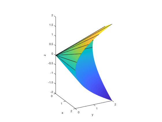
Figure 4: The $2\times 2$ semidefinite cone

Definition 3.

Suppose $K$ is a closed convex cone, $H$ is an affine subspace, and $H\cap K\neq\emptyset.$ We define the minimal cone of $H\cap K$ as the smallest face of $K$ that contains $H\cap K.$

We define the minimal cone of ($P$), of ($D$) and of ($HD$) as the minimal cone of their feasible sets. In particular, the minimal cone of ($P$) is the minimal cone of $(\operatorname{lin}\{\,A_{1},\dots,A_{m}\}+B)\cap{\cal S}_{+}^{n}.$

The following easy-to-verify fact will help us identify the minimal cone of SDPs: if $H\subseteq{\cal S}^{n}$ is an affine subspace which contains a psd matrix, then the minimal cone of $H\cap{\cal S}_{+}^{n}$ is the smallest face of ${\cal S}_{+}^{n}$ that contains the maximum rank psd matrix of $H.$

Example 5.

Let $H$ be the linear subspace spanned by the matrices

$$A_{1}=\begin{pmatrix}1&\phantom{0}&\phantom{0}\\ \phantom{0}&0&\phantom{0}\\ \phantom{0}&\phantom{0}&0\end{pmatrix},\,A_{2}=\begin{pmatrix}\phantom{0}&\phantom{0}&1\\ \phantom{0}&1&\phantom{0}\\ 1&\phantom{0}&\phantom{0}\end{pmatrix},$$

and $K={\cal S}_{+}^{3}.$

Then $H\cap K=\{\lambda A_{1}:\lambda\geq 0\},\,$ hence this latter set is the minimal cone of $H\cap K.$

In this paper we are mostly interested in the minimal cone of ($D$) and of ($HD$) .

Example 6.

(Example 1 continued) In this example we proved that in any feasible solution of ($D$) the first row and column is zero. Thus

$$Y\,=\,\begin{pmatrix}0&\phantom{0}&\phantom{0}\\ \phantom{0}&1&\phantom{0}\\ \phantom{0}&\phantom{0}&1\end{pmatrix}$$ (4.32)

is a maximum rank feasible solution in ($D$), so the minimal cone of ($D$) is $0\oplus{\cal S}_{+}^{2}.$

Why is the minimal cone interesting? Suppose $F$ is the minimal cone of ($D$). Then there is a feasible $Y$ in the relative interior of $F,$ otherwise the feasible set of ($D$) would be contained in a smaller face of ${\cal S}_{+}^{n}.$ Thus replacing the primal constraint by $B-\sum_{i}x_{i}A_{i}\in F^{*}$ yields a primal-dual pair with no duality gap and primal attainment. (An analogous result holds for the minimal cone of ($P$) and enlarging the dual feasible set). For details, see e.g. [13].

How do we actually compute the minimal cone of $H\cap K$? The following basic facial reduction algorithm is designed for this task.

Algorithm 1 Facial Reduction

Let $F_{0}=K,\,i=1.$

for ${i=1,2,\dots}$ do

     Choose $y_{i}\in F_{i-1}^{*}\cap H^{\perp}.$

     Let $F_{i}=F_{i-1}\cap y_{i}^{\perp}.$

end for

Definition 4.

We say that a sequence $(y_{1},\dots,y_{k})$ output by Algorithm 1 is a facial reduction sequence for $K;$ and we say that it is a strict facial reduction sequence for $K$ if in addition $y_{i}\in F_{i-1}^{*}\setminus F_{i-1}^{\perp}$ for all $i\geq 1.$

We denote the set of facial reduction sequences for $K$ by $\operatorname{FR}(K).$

Suppose that $(y_{1},\dots,y_{k})$ is constructed by Algorithm 1. Then all $F_{i}$ contain $H\cap K,\,$ and hence they also contain the minimal cone of $H\cap K.$ Further, there is always a possible output $(y_{1},\dots,y_{k})$ such that $F_{k}$ is the minimal cone, see e.g., [13]. We will say that such a sequence defines the minimal cone of $H\cap K.$

Clearly, Algorithm 1 can generate many possible sequences (it can even choose several $y_{i}$ which are zero), but it is best to terminate it in a minimim number of steps.

Definition 5.

Suppose $H$ is an affine subspace with $H\cap K\neq\emptyset.$ The singularity degree $d(H\cap K)$ of $H\cap K$ is the smallest number of steps necessary for Algorithm 1 to construct the minimal cone of $H\cap K.$

The singularity degrees of ($P$), ($D$), and ($HD$) are defined as the singularity degree of their feasible sets. They are denoted by $d\eqref{p},\,d\eqref{d},\,$ and $d\eqref{HD},\,$ respectively.

The singularity degree of SDPs was introduced in the seminal paper [29]. It was used to bound the distance of a symmetric matrix from $H\cap{\cal S}_{+}^{n},\,$ given the distances from $H$ and from ${\cal S}_{+}^{n}.$ More recently it was used in [6] to bound the rate of convergence of the alternating projection algorithm to such a set.

For later reference, we state a basic bound on the singularity degree (for details, see, e.g., [13, Theorem 1]):

$$d(H\cap K)\leq\dim H^{\perp}.$$ (4.33)

In the following examples involving SDPs we denote the members of facial reduction sequences by capital letters (since they are matrices).

Example 7.

(Example 5 continued) In this example the sequence $(Y_{1},Y_{2})$ below defines the minimal cone, with corresponding faces shown. Note that $F_{2}$ is the minimal cone.

$$Y_{1} = \begin{pmatrix}0&0&0\\ 0&0&0\\ 0&0&1\end{pmatrix},\,F_{1}\,=\,{\cal S}_{+}^{3}\cap Y_{1}^{\perp}\,=\,\begin{pmatrix}\parbox{28.45274pt}{$\,\,\bigoplus$}&\parbox{11.38092pt}{$\begin{array}[]{c}0\\ 0\end{array}$}\\ \parbox{28.45274pt}{$0\,\,\,\,\,\,0$}&0\hskip 11.38092pt\end{pmatrix},$$

$$Y_{2} = \begin{pmatrix}0&0&-1\\ 0&2&0\\ -1&0&0\end{pmatrix},F_{2}\,=\,F_{1}\cap Y_{2}^{\perp}\,=\,\begin{pmatrix}\oplus&0&0\\ 0&0&0\\ 0&0&0\end{pmatrix}.$$

Since $Y_{1}$ is the maximum rank psd matrix in $H^{\perp},\,$ it is the best choice to start such a facial reduction sequence, hence $d(H\cap{\cal S}_{+}^{3})=2.$

Example 8.

(Example 1 and 6 continued) In this example the minimal cone of ($D$) is $0\oplus{\cal S}_{+}^{2}$ and $A_{1}\bullet Y=0$ implies $Y\in 0\oplus{\cal S}_{+}^{2}.$ Since $A_{1}\succeq 0,\,$ the one element facial reduction sequence $(A_{1})$ defines the minimal cone of ($D$).

The reader may wonder, why we connect positive gaps to the singularity degree of ($D$) and of $(HD),\,$ and not to the singularity degree of $(P).$ We could do the latter, by exchanging the roles of the primal and dual. However, we think that our treatment is more intuitive, as we next explain.

The dual feasible set is $H\cap{\cal S}_{+}^{n},\,$ where

$$\begin{array}[]{rcl}H&=&\{\,Y\in{\cal S}^{n}\,|\,A_{i}\bullet Y=c_{i}\,\forall i\,\}\\ &=&\{\,Y\in{\cal S}^{n}\,|\,A_{i}\bullet Y=0\,\forall i\,\}+Y_{0},\end{array}$$ (4.34)

where $Y_{0}\in H$ is arbitrary. Thus, to define the minimal cone of ($D$) we use a facial reduction sequence whose members are in $H^{\perp}\subseteq\operatorname{lin}\{A_{1},\dots,A_{m}\ \}.$ As we will show, in our instances actually the $A_{i}$ themselves form a facial reduction sequence that defines the minimal cone of ($D$), and this makes the essential structure of the minimal cone apparent. An analogous statement holds for the minimal cone of $(HD).$

4.2 The singularity degree of the single sequence SDPs in Example 2

We now analyze the singularity degree of the duals of the SDPs given in Example 2.

Theorem 2.

Let ($D$) be the dual of the SDP (3.20). Then

$$d(D)=m-1.$$

Proof Recall that $m=n-1$ in this SDP. We first claim that the minimal cone of ($D$) is $0\oplus{\cal S}_{+}^{2}.$ Indeed, by the argument in (3.21) the minimal cone is contained in $0\oplus{\cal S}_{+}^{2}.$ Since $0\oplus I_{2}$ is feasible in ($D$), the minimal cone is exactly $0\oplus{\cal S}_{+}^{2}.$

An analogous argument (by plugging $Y\succeq 0$ into the equations $A_{1}\bullet Y=0,\,\dots,\,A_{i}\bullet Y=0$, like in (3.21)) proves

$${\cal S}_{+}^{n}\cap A_{1}^{\perp}\cap\dots\cap A_{i}^{\perp}\,=\,0_{i}\oplus{\cal S}_{+}^{n-i}\;{\rm for}\;1\leq i\leq m-1.$$ (4.35)

Let $i\in\{1,\dots,m-1\}.$ Then clearly $A_{i+1}\in(0_{i}\oplus{\cal S}_{+}^{n-i})^{*},\,$ so by (4.35) we deduce

$$A_{i+1}\in({\cal S}_{+}^{n}\cap A_{1}^{\perp}\cap\dots\cap A_{i}^{\perp})^{*},$$

hence $(A_{1},\dots,A_{m-1})$ is a facial reduction sequence, which defines the minimal cone of $(D).\,$ Thus $d(D)\leq m-1.$

To complete the analysis we show that any strict facial reduction sequence in $\operatorname{lin}\,\{A_{1},\dots,A_{m}\}$ reduces ${\cal S}_{+}^{n}$ by at most as much as the $A_{i}$ themselves. This is done in Claim 1, whose proof is in Appendix A.2.

Claim 1.

Suppose $i\in\{1,\dots,m-1\}$ and $(Y_{1},\dots,Y_{i})$ is a strict facial reduction sequence, whose members are all in $\operatorname{lin}\{A_{1},\dots,A_{m}\}.$ Then

$${\cal S}_{+}^{n}\cap Y_{1}^{\perp}\cap\dots\cap Y_{i}^{\perp}\,=\,0_{i}\oplus{\cal S}_{+}^{n-i}.$$ (4.36)

Having Claim 1 at hand, let $(Y_{1},\dots,Y_{i})$ be a strict facial reduction sequence that defines the minimal cone of ($D$). Since the minimal cone is $0_{n-2}\oplus{\cal S}_{+}^{2},$ by Claim 1 we deduce $i=n-2=m-1.$ Hence $d(\ref{d})=m-1,$ and the desired result follows. ∎

4.3 The singularity degree of the double sequence SDPs in Example 4

We now turn to studying the singularity degrees of the duals of the SDPs in Example 4. The main rationale for creating these SDPs in the first place is that the singularity degrees of two associated duals achieve an upper bound.

Theorem 3.

Let ($D$) be the dual of (3.25) and ($HD$) its homogeneous dual. Then

$$d\eqref{d}=m-1\,\,{\rm and}\,\,d\eqref{HD}=m.$$

Proof sketch Recall that $n=2m+1$ in this example. The proof of $d\eqref{d}=m-1$ is almost verbatim the same as the proof of the same statement in Theorem 2: the key is that for $i\in\{1,\dots,m-1\}$

$$\begin{array}[]{rcl}{\cal S}_{+}^{n}\cap A_{1}^{\perp}\cap\dots\cap A_{i}^{\perp}&=&\{\;Y\succeq 0\;|\;{\rm\;rows\;and\;columns\;of\;}Y{\rm\;indexed\;by}\\ &&\;\;\;\;\;\;\;\;\;\;\;\;\;\;\;\;\;1,\dots,i{\rm\;and\;}m+1,\dots,m+i\;{\rm are\;zero\;}\}\end{array}$$

(cf. (3.27)). We leave the details to the reader.

We next outline the proof of $d\eqref{HD}=m.$ The argument goes like this: when we check whether $Y\succeq 0$ is feasible in ($HD$), it suffices (and is convenient) to plug $Y$ into the equations

$$B\bullet Y=0,\,A_{2}\bullet Y=0,\dots,A_{m}\bullet Y=0$$

in this order. Indeed, $B\bullet Y=0$ implies that the first $m+1$ rows and columns of $Y$ are zero, and this implies $A_{1}\bullet Y=0,$ so we do not have to check this last equation separately. Then $A_{2}\bullet Y=0$ implies that the $(m+2)$nd row and column of $Y$ is zero, and so on.

Thus,

$${\cal S}_{+}^{n}\cap B^{\perp}\cap A_{2}^{\perp}\cap\dots\cap A_{i}^{\perp}\,=\,0_{m+i}\oplus{\cal S}_{+}^{m-i+1}\,\,{\rm for\,}i=2,\dots,m.$$ (4.37)

Equation (4.37) with $i=m$ implies that the minimal cone of ($HD$) is contained in $0\oplus{\cal S}_{+}^{1}.$ Since $0\oplus I_{1}$ is feasible in ($HD$), the minimal cone is exactly $0\oplus{\cal S}_{+}^{1}.$

Equation (4.37) also implies that $(B,A_{2},\dots,A_{m-1},-A_{m})$ is a facial reduction sequence that defines the minimal cone of ($HD$). Consequently, $d\eqref{HD}\leq m.$

We can prove $d\eqref{HD}=m$ by using Claim 2 below, whose proof is very similar to the proof of Claim 1, so it is omitted.

Claim 2.

Suppose $i\in\{1,\dots,m\}$ and $(Y_{1},\dots,Y_{i})$ is a strict facial reduction sequence, whose members are all in $\operatorname{lin}\,\{\,B,A_{2},\dots,A_{m}\,\}.$ Then

$${\cal S}_{+}^{n}\cap Y_{1}^{\perp}\cap\dots\cap Y_{i}^{\perp}\,=\,0_{m+i}\oplus{\cal S}_{+}^{m-i+1}.$$

Given Claim 2 the proof of Theorem 3 is complete. ∎

5 Maximal singularity degree implies zero duality gap

We now show that the SDPs of Section 3 are, in a well defined sense, the best possible: we prove that

$$d\eqref{d}\leq m,\,{\rm and}\,d\eqref{HD}\leq m+1\,$$

always hold, and when these upper bounds are attained, there is no gap. For the reader’s sake we present our results in two subsections.

5.1 Maximal singularity degree of ($D$) implies zero duality gap

The main result of this subsection is fairly straightforward.

Proposition 2.

The inequality

$$d\eqref{d} \leq m.$$

always holds, and when $d\eqref{d}=m\,$ there is no duality gap.

Proof Let $H$ and $Y_{0}$ be as in (4.34). We see that

$$H^{\perp}\,=\,\operatorname{lin}\{\,A_{1},\dots,A_{m}\,\}\cap Y_{0}^{\perp}.$$ (5.38)

Since the feasible set of ($D$) is $H\cap{\cal S}_{+}^{n},\,$ we deduce

$$d\eqref{d}\leq\dim H^{\perp}\,\leq\,m,$$

where the first inequality comes from (4.33) and the second from (5.38).

Suppose $d\eqref{d}=m.$ Then $\dim H^{\perp}=m,\,$ hence $c_{i}=A_{i}\bullet Y_{0}=0\,$ for all $i.\,$ So the objective function in ($P$) is $c=0,\,$ and this proves that there is no gap. ∎

5.2 Maximal singularity degree of ($HD$) implies zero duality gap

We first observe that (4.33) with $H=\{\,Y\,:\,B\bullet Y=A_{i}\bullet Y=0\,\forall i\,\}$ implies

$$d\eqref{HD}\leq m+1.$$ (5.39)

The main result of this subsection is

Theorem 4.

Suppose $d\eqref{HD}=m+1.\,$ Then the only feasible solution of ($P$) is $x=0,\,$ and ($D$) is strictly feasible. Hence

$$\operatorname{val}(\ref{p})=\operatorname{val}(\ref{d})=0.$$

∎

To prove Theorem 4, we first we define certain structured facial reduction sequences for ${\cal S}_{+}^{n}.$ These sequences were originally introduced in [13].

Definition 6.

We say that $(M_{1},\dots,M_{k})$ is a regularized facial reduction sequence for ${\cal S}_{+}^{n}$ if $M_{i}$ is of the form

$$M_{i}=\bordermatrix{&\overbrace{\qquad\qquad\qquad}^{\textstyle r_{1}+\ldots+r_{i-1}}&\overbrace{\qquad}^{\textstyle r_{i}}&\overbrace{\qquad\qquad\qquad\quad}^{\textstyle n-r_{1}-\ldots-r_{i}}\cr\\ &\times&\times&\times\cr&\times&I&0\cr&\times&0&0\cr}\in{\cal S}^{n}$$

for $i=1,\dots,k,\,$ where the $r_{i}$ are nonnegative integers, and the $\times$ symbols correspond to blocks with arbitrary elements.

For instance, $(A_{1},\dots,A_{m})$ in the single sequence SDPs in Example 2 is a regularized facial reduction sequence. We refer to Figure 2 in which the identity blocks in the $A_{i}$ are red, and the blocks with arbitrary elements are blue. Also, $(B,A_{2},\dots,A_{m-1},-A_{m})$ is a regularized facial reduction sequence in the double sequence SDPs in Example 4.

Lemma 2.

Suppose $d\eqref{HD}=m+1.$ Then ($P$) has a reformulation

$$\begin{array}[]{rcl}\sup\sum_{i=1}^{m}c_{i}^{\prime}x_{i}&&\\ \sum_{i=1}^{m}x_{i}A_{i}^{\prime}&\preceq&B\,=\,\begin{pmatrix}I_{r}&0\\ 0&0\end{pmatrix}\end{array} P^{\prime}$$ ()

in which $(B,A_{1}^{\prime},\dots,A_{m}^{\prime})$ is a regularized facial reduction sequence. Furthermore, ($P^{\prime}$) can be constructed using only operations (2), (3) and (4) in Definition 1.

The proof of Lemma 2 is a bit technical, so we give in Appendix A.3. However, we next illustrate it.

Example 9.

Consider the SDP

$$\begin{array}[]{llcl}\sup&13x_{1}-3x_{2}\\ s.t.&x_{1}\begin{pmatrix}0&&2&2\\ &1&&\\ 2&&0&\\ 2&&&0\end{pmatrix}+x_{2}\begin{pmatrix}0&&&\\ &0&&2\\ &&1&\\ &2&&0\end{pmatrix}\preceq\begin{pmatrix}1&&&\\ &0&&\\ &&0&\\ &&&0\end{pmatrix},\end{array}$$ (5.40)

and let $A_{1}$ and $A_{2}$ denote the matrices on the left hand side, and $B$ the right hand side. Then

• $B$ is the maximum rank slack and (5.40) is in the form of ($P^{\prime}$).

• $(B,A_{1},A_{2})$ is a regularized facial reduction sequence, which defines the minimal cone of $(HD),\,$ which is $0\oplus{\cal S}_{+}^{1},\,$ i.e., the set of nonnegative multiples of

  $$Y=\begin{pmatrix}0&0&0&0\\ 0&0&0&0\\ 0&0&0&0\\ 0&0&0&1\end{pmatrix}.$$

Thus $d(\mbox{\ref{HD}})\leq 3$ and we claim that actually

$$d(\mbox{\ref{HD}})=3\,{\rm holds.}$$

Indeed, let $L:=\operatorname{lin}\,\{B,A_{1},\dots,A_{m}\},$ then the facial reduction sequences that define the minimal cone of ($HD$) are in $L.$

Clearly, $B$ is the only nonzero psd matrix in $L.$ Further, $A_{1}$ is the only matrix in $L\cap({\cal S}_{+}^{3}\cap B^{\perp})^{*}$ whose lower right $3\times 3$ block is nonzero, thus $(B,A_{1})$ is the only strict length two facial reduction sequence in $L.$ By similar logic $(B,A_{1},A_{2})$ is the only strict length three facial reduction sequence in $L.$

Thus $d\eqref{HD}=3,$ as desired.

We need some more notation: for $Y\in{\cal S}^{n}$ and $\mathcal{I},\mathcal{J}\subseteq\{1,\dots,n\}$ we define $Y(\mathcal{I},\mathcal{J})$ as the submatrix of $Y$ with rows in $\mathcal{I}$ and columns in $\mathcal{J},$ and let

$$Y(\mathcal{I}) := Y(\mathcal{I},\mathcal{I}).$$

Proof of Theorem 4: Assume $d\eqref{HD}=m+1.$ Clearly, we can assume that ($P$) was reformulated into the form of ($P^{\prime}$): as Lemma 2 shows, this can be done using only operations (2), (3) and (4) in Definition 1, and under these operations the statements of Theorem 4 are invariant.

So we assume that ($P$) is the same as ($P^{\prime}$), and we denote the constraint matrices on the left by $A_{i}$ for $i=1,\dots,m.$ For brevity, let $A_{0}:=B.$

Assume that in ($P$) the regularized facial reduction sequence $(A_{0},A_{1},\dots,A_{m})$ has block sizes $r_{0},r_{1},\dots,r_{m}.$ Define the index sets

$$\mathcal{I}_{0} := \{1,\dots,r_{0}\},$$

$$\mathcal{I}_{1} := \{r_{0}+1,\dots,r_{0}+r_{1}\},$$

$$\vdots$$

$$\mathcal{I}_{m} := \{\sum_{i=1}^{m-1}r_{i}+1,\dots,\sum_{i=1}^{m}r_{i}\}.$$

Further, for $i\leq j$ we let

$$\mathcal{I}_{i:j} := \mathcal{I}_{i}\cup\dots\cup\mathcal{I}_{j},$$

and $\mathcal{I}_{m+1}:=\{1,\dots,n\}\setminus\mathcal{I}_{1:m}.$ Finally, we write $\mathcal{I}_{i:}$ for $\mathcal{I}_{i:(m+1)}$ for all $i$ (we can do this without confusion, since $m+1$ is the largest index).

We first prove

$$A_{i}(\mathcal{I}_{i-1},\mathcal{I}_{(i+1):})\neq 0\,\,{\rm for}\,\,i=1,\dots,m.$$ (5.41)

Let $i\in\{1,\dots,m\}$ and let us picture $A_{i-1}$ and $A_{i}$ in equation (5.42): as always, the empty blocks are zero, and the $\times$ blocks are arbitrary. The blocks marked by $\otimes$ are $A_{i}(\mathcal{I}_{i-1},\mathcal{I}_{(i+1):})$ and its symmetric counterpart.

$$A_{i-1}\,=\,\begin{pmatrix}[c|c|c|c]\makebox[0.0pt][l]{$\smash{\overbrace{\phantom{\begin{matrix}\mbox{$\,\,\,\,\times\,\,\,\,$}\end{matrix}}}^{\text{$\mathcal{I}_{0:(i-2)}$}}}$}\mbox{$\,\,\,\,\times\,\,\,\,$}&\makebox[0.0pt][l]{$\smash{\overbrace{\phantom{\begin{matrix}\mbox{$\,\,\times\,\,$}\end{matrix}}}^{\text{$\mathcal{I}_{i-1}$}}}$}\mbox{$\,\,\times\,\,$}&\makebox[0.0pt][l]{$\smash{\overbrace{\phantom{\begin{matrix}\mbox{$\,\,\times\,\,$}\end{matrix}}}^{\text{$\mathcal{I}_{i}$}}}$}\mbox{$\,\,\times\,\,$}&\makebox[0.0pt][l]{$\smash{\overbrace{\phantom{\begin{matrix}\mbox{$\,\,\,\,\times\,\,\,\,\,$}\end{matrix}}}^{\text{$\mathcal{I}_{(i+1):}$}}}$}\mbox{$\,\,\,\,\times\,\,\,\,\,$}\\ \hline\cr\times&I&&\\ \hline\cr\times&&&\\ \hline\cr\times&\phantom{0}&&\end{pmatrix},\,A_{i}\,=\,\begin{pmatrix}[c|c|c|c]\makebox[0.0pt][l]{$\smash{\overbrace{\phantom{\begin{matrix}\mbox{$\,\,\,\,\times\,\,\,\,$}\end{matrix}}}^{\text{$\mathcal{I}_{0:(i-2)}$}}}$}\mbox{$\,\,\,\,\times\,\,\,\,$}&\makebox[0.0pt][l]{$\smash{\overbrace{\phantom{\begin{matrix}\mbox{$\,\,\times\,\,$}\end{matrix}}}^{\text{$\mathcal{I}_{i-1}$}}}$}\mbox{$\,\,\times\,\,$}&\makebox[0.0pt][l]{$\smash{\overbrace{\phantom{\begin{matrix}\mbox{$\,\,\times\,\,$}\end{matrix}}}^{\text{$\mathcal{I}_{i}$}}}$}\mbox{$\,\,\times\,\,$}&\makebox[0.0pt][l]{$\smash{\overbrace{\phantom{\begin{matrix}\mbox{$\,\,\,\,\times\,\,\,\,\,$}\end{matrix}}}^{\text{$\mathcal{I}_{(i+1):}$}}}$}\mbox{$\,\,\,\,\times\,\,\,\,\,$}\\ \hline\cr\times&\times&\times&\otimes\\ \hline\cr\times&\times&I&\\ \hline\cr\times&\otimes&&\end{pmatrix}.$$ (5.42)

Now suppose the $\otimes$ blocks are zero and let $A_{i-1}^{\prime}:=\lambda A_{i-1}+A_{i}$ for some large $\lambda>0.$ Then by the Schur complement condition for positive definiteness we find

$$A_{i-1}^{\prime}(\mathcal{I}_{(i-1):i})\succ 0,$$

hence $(A_{1},\dots,A_{i-2},A_{i-1}^{\prime},A_{i+1},\dots,A_{m})$ is a shorter facial reduction sequence, which also defines the minimal cone of ($HD$). Thus $d\eqref{HD}\leq m,\,$ which is a contradiction. We thus proved (5.41).

We illustrate statement (5.41) in equation (5.43), when $m=2$ and $d\eqref{HD}=3:$ the $\otimes$ blocks in $A_{1}$ and $A_{2}$ were just proven to be nonzero.

$$A_{0}=\begin{tabular}[]{|m{14pt}|m{14pt}|m{14pt}|m{14pt}|}\lx@intercol\hfil \leavevmode\hbox to14pt{\vbox to3.22pt{\text{[drawing]}}}\hfil\lx@intercol &\lx@intercol\hfil \leavevmode\hbox to14pt{\vbox to3.22pt{\text{[drawing]}}}\hfil\lx@intercol &\lx@intercol\hfil \leavevmode\hbox to14pt{\vbox to3.22pt{\text{[drawing]}}}\hfil\lx@intercol &\lx@intercol\hfil \leavevmode\hbox to14pt{\vbox to3.22pt{\text{[drawing]}}}\hfil\lx@intercol\\ \hline\cr\vrule\lx@intercol\hfil$I$\hfil\lx@intercol\vrule\lx@intercol &&&\\ \hline\cr&&&\\ \hline\cr&&&\\ \hline\cr&&&\\ \hline\cr\end{tabular}\leavevmode\hbox to18.4pt{\vbox to18.7pt{\text{[drawing]}}}\leavevmode\hbox to18.4pt{\vbox to18.7pt{\text{[drawing]}}}\leavevmode\hbox to18.4pt{\vbox to18.7pt{\text{[drawing]}}}\leavevmode\hbox to18.4pt{\vbox to18.7pt{\text{[drawing]}}}\,,\,\,\,A_{1}=\begin{tabular}[]{|m{14pt}|m{14pt}|m{14pt}|m{14pt}|}\lx@intercol\hfil \leavevmode\hbox to14pt{\vbox to3.22pt{\text{[drawing]}}}\hfil\lx@intercol &\lx@intercol\hfil \leavevmode\hbox to14pt{\vbox to3.22pt{\text{[drawing]}}}\hfil\lx@intercol &\lx@intercol\hfil \leavevmode\hbox to17pt{\vbox to3.22pt{\text{[drawing]}}}\hfil\lx@intercol &\lx@intercol\hfil \leavevmode\hbox to14pt{\vbox to3.22pt{\text{[drawing]}}}\hfil\lx@intercol\\ \hline\cr\vrule\lx@intercol\hfil$\times$\hfil\lx@intercol\vrule\lx@intercol &\lx@intercol\hfil$\times$\hfil\lx@intercol\vrule\lx@intercol &\lx@intercol\hfil$\otimes$\hfil\lx@intercol\vrule\lx@intercol\\ \hline\cr\vrule\lx@intercol\hfil$\times$\hfil\lx@intercol\vrule\lx@intercol &\lx@intercol\hfil$I$\hfil\lx@intercol\vrule\lx@intercol &&\\ \hline\cr\hbox{\multirowsetup$\otimes$}&&&\\ \cline{2-4}\cr&&&\\ \hline\cr\end{tabular}\leavevmode\hbox to18.4pt{\vbox to18.7pt{\text{[drawing]}}}\leavevmode\hbox to18.4pt{\vbox to18.7pt{\text{[drawing]}}}\leavevmode\hbox to21.4pt{\vbox to18.7pt{\text{[drawing]}}}\leavevmode\hbox to18.4pt{\vbox to18.7pt{\text{[drawing]}}}\,,\,\,\,A_{2}=\begin{tabular}[]{|m{14pt}|m{14pt}|m{14pt}|m{14pt}|}\lx@intercol\hfil \leavevmode\hbox to14pt{\vbox to3.22pt{\text{[drawing]}}}\hfil\lx@intercol &\lx@intercol\hfil \leavevmode\hbox to14pt{\vbox to3.22pt{\text{[drawing]}}}\hfil\lx@intercol &\lx@intercol\hfil \leavevmode\hbox to17pt{\vbox to3.22pt{\text{[drawing]}}}\hfil\lx@intercol &\lx@intercol\hfil \leavevmode\hbox to14pt{\vbox to3.22pt{\text{[drawing]}}}\hfil\lx@intercol\\ \hline\cr\vrule\lx@intercol\hfil$\times$\hfil\lx@intercol\vrule\lx@intercol &\lx@intercol\hfil$\times$\hfil\lx@intercol\vrule\lx@intercol &\lx@intercol\hfil$\times$\hfil\lx@intercol\vrule\lx@intercol &\lx@intercol\hfil$\times$\hfil\lx@intercol\vrule\lx@intercol \\ \hline\cr\vrule\lx@intercol\hfil$\times$\hfil\lx@intercol\vrule\lx@intercol &\lx@intercol\hfil$\times$\hfil\lx@intercol\vrule\lx@intercol &\lx@intercol\hfil$\times$\hfil\lx@intercol\vrule\lx@intercol &\lx@intercol\hfil$\otimes$\hfil\lx@intercol\vrule\lx@intercol \\ \hline\cr\vrule\lx@intercol\hfil$\times$\hfil\lx@intercol\vrule\lx@intercol &\lx@intercol\hfil$\times$\hfil\lx@intercol\vrule\lx@intercol &\lx@intercol\hfil$I$\hfil\lx@intercol\vrule\lx@intercol &\\ \hline\cr\vrule\lx@intercol\hfil$\times$\hfil\lx@intercol\vrule\lx@intercol &\lx@intercol\hfil$\otimes$\hfil\lx@intercol\vrule\lx@intercol &&\\ \hline\cr\end{tabular}\leavevmode\hbox to18.4pt{\vbox to18.7pt{\text{[drawing]}}}\leavevmode\hbox to18.4pt{\vbox to18.7pt{\text{[drawing]}}}\leavevmode\hbox to21.4pt{\vbox to18.7pt{\text{[drawing]}}}\leavevmode\hbox to18.4pt{\vbox to18.7pt{\text{[drawing]}}} \mathcal{I}_{0} \mathcal{I}_{1} \mathcal{I}_{2} \mathcal{I}_{3} \mathcal{I}_{0} \mathcal{I}_{1} \mathcal{I}_{2} \mathcal{I}_{3} \mathcal{I}_{0} \mathcal{I}_{1} \mathcal{I}_{2} \mathcal{I}_{3} \mathcal{I}_{0} \mathcal{I}_{1} \mathcal{I}_{2} \mathcal{I}_{3} \mathcal{I}_{0} \mathcal{I}_{1} \mathcal{I}_{2} \mathcal{I}_{3} \mathcal{I}_{0} \mathcal{I}_{1} \mathcal{I}_{2} \mathcal{I}_{3}$$ (5.43)

We next prove that the only feasible solution of ($P$) is $x=0.$ For that, let $x$ be feasible in ($P$) and define

$$Z=A_{0}-\sum_{i=1}^{m}x_{i}A_{i}.$$

Since $A_{i}(\mathcal{I}_{m+1})=0$ for all $i,\,$ we deduce $Z(\mathcal{I}_{m+1})=0.$ Since $Z\succeq 0,\,$ we deduce that the columns of $Z$ corresponding to $\mathcal{I}_{m+1}$ are zero. Hence

$$0\,=\,Z(\mathcal{I}_{m-1},\mathcal{I}_{m+1})\,=\,x_{m}\underbrace{A_{m}(\mathcal{I}_{m-1},\mathcal{I}_{m+1})}_{\neq 0},$$

so $x_{m}=0,$ which in turn implies $Z(\mathcal{I}_{m:(m+1)})=0.$ By a similar reasoning,

$$0\,=\,Z(\mathcal{I}_{m-2},\mathcal{I}_{m:(m+1)})\,=\,x_{m-1}\underbrace{A_{m-1}(\mathcal{I}_{m-2},\mathcal{I}_{m:(m+1)})}_{\neq 0},$$

hence $x_{m-1}=0,$ and so on. Thus $x=0$ follows, as wanted.

We finally prove that ($D$) is strictly feasible. By condition (5.41) the $A_{i}$ are linearly independent, so there exists $\bar{Y}\in{\cal S}^{n}$ such that $A_{i}\bullet\bar{Y}=c_{i}\,$ for all $i.$

By an argument analogous to the previuous one, we see that the only psd linear combination of the $A_{i}$ is the zero matrix. Thus the Gordan-Stiemke theorem (1.2) with

$$H:=\operatorname{lin}\,\{\,A_{1},\dots,A_{m}\,\}$$

implies that there is $\hat{Y}\succ 0$ such that $A_{i}\bullet\hat{Y}=0$ for $i=1,\dots,m.$ Clearly, if $\lambda>0$ is large enough, then $Y:=\bar{Y}+\lambda\hat{Y}$ is strictly feasible in ($D$).

The proof is now complete.

∎

Example 10.

(Example 9 continued) Recall that in this SDP we have $d\eqref{HD}=3.$ We chose the blocks specified in equation (5.41) to have entries all equal to $2.$ Note that $\mathcal{I}_{0}=\{1\},\,\mathcal{I}_{1}=\{2\},\,\mathcal{I}_{2}=\{3\}.$

A possible $Y$ that is strictly feasible in ($D$) is

$$Y\,=\,(y_{ij})_{i,j=1}^{4}\,=\,\begin{pmatrix}1&0&2&1\\ 0&1&0&-2\\ 2&0&5&0\\ 1&-2&0&25\end{pmatrix}.$$

It is worth to elaborate on Theorem 4 some more. By the Gordan-Stiemke theorem (1.2) the dual ($D$) is strictly feasible iff its singularity degree is $0.$ Thus Theorem 4 establishes the following surprising implication:

$$d\eqref{HD}=m\,\Rightarrow\,d\eqref{d}=0.$$ (5.44)

6 A computational study

This section presents a computational study of SDPs with positive duality gaps.

We first remark that pathological SDPs are extremely difficult to solve by interior point methods. However, some recent implementations of facial reduction [24, 36] work on some pathological SDPs. We refer to [15] for an implementation of the Douglas-Rachford splitting algorithm to solve the weakly infeasible SDPs from [15] and to [10] for a homotopy method to tackle these same SDPs. Furthermore, the exact SDP solver SPECTRA [11] can solve small SDPs in exact arithmetic. We hope that the detailed study we present here will inspire further research.

We generated a library of challenging SDPs based on the single sequence SDPs in Example 2 and Example 3.

First we created SDPs described in Example 2 with $m=2,\dots,11.$ We multiplied the primal objective by $10,\,$ meaning we chose

$$c=10e_{m}.$$

(Recall $m=n-1.$) Thus in these instances the primal optimal value is still zero, but the dual optimal value is $10.$

Second, we constructed single sequence SDPs as given in Example 3, with $m=2,\dots,11.$ For consistency, we multiplied the primal objective by $10,\,$ to make it $10e_{m}.$ Then the primal optimal value is still zero, and the dual is still infeasible, so the duality gap is still infinity. (Recall from Proposition 1 that the dual is weakly infeasible.)

We say that the SDPs thus created from Examples 2 and 3 are clean, meaning the duality gap can be verified by simple inspection.

To construct SDPs in which the duality gap is less obvious, we added an optional

• Messing step: Let $T$ be an invertible matrix with integer entries, and replace all $A_{i}$ by $T^{T}A_{i}T$ and $B$ by $T^{T}BT.$

Thus we have four categories of SDPs, stored under the names

• ${\mathit{g}ap}\_{\mathit{s}ingle}\_{\mathit{f}inite}\_{\mathit{c}lean}\_m,\,$

• ${\mathit{g}ap}\_{\mathit{s}ingle}\_{\mathit{f}inite}\_{\mathit{m}essy}\_m,\,$

• ${\mathit{g}ap}\_{\mathit{s}ingle}\_{\mathit{i}nf}\_{\mathit{c}lean}\_m,$ and

• ${\mathit{g}ap}\_{\mathit{s}ingle}\_{\mathit{i}nf}\_{\mathit{m}essy}\_m,$

where $m=2,\dots,11$ in each category. We tested two SDP solvers: the Mosek commercial solver, and the SDPA-GMP high precision SDP solver [9].

Table 1 reports the number of correctly solved instances in each category.

The solvers are not designed to detect a finite positive duality gap. Thus, to be fair, we report that an SDP with a finite duality gap was correctly solved when Mosek does not report “OPTIMAL” or “NEAROPTIMAL” status, and SDPA-GMP does not report “pdOPT” status . The solvers, however, are designed to detect infeasibility, and in the instances with infinite duality gap the dual is infeasible. Hence we would report that an instance is correctly solved, when Mosek or SDPA-GMP report dual infeasibility. However, this did not happen for any of the instances.

We also tested the preprocessing method of [24] and Sieve-SDP [36] on the dual problems, then on the preprocessed problems we ran Mosek. Both these methods correctly preprocessed all “clean” instances, but could not preprocess the “messy” instances. See the rows in Table 1 marked by PP+Mosek and Sieve-SDP+Mosek.

	Gap, single, finite		Gap, single, infinite
	Clean	Messy	Clean	Messy
Mosek	1	1	0	0
SDPA-GMP	1	1	0	0
PP+Mosek	10	1	10	0
Sieve-SDP + Mosek	10	1	10	0

Table 1: Computational results

We finally tested the exact SDP solver SPECTRA [11] on the ${\mathit{g}ap}\_{\mathit{s}ingle}\_{\mathit{f}inite}\_{\mathit{m}essy}\_2$ instance. SPECTRA cannot run on our SDPs as they are, since they do not satisfy an important algebraic assumption. However, SPECTRA could compute and certify in exact arithmetic the optimal solution of the perturbed dual

$$\begin{array}[]{rl}\inf&B\bullet Y\\ s.t.&A_{i}\bullet(Y+\epsilon I)\,=\,\,c_{i}(i=1,2)\\ &Y\succeq 0\end{array}$$ (6.45)

where $\epsilon$ was chosen as a small rational number.

For example, with $\epsilon=10^{-200}$ SPECTRA found and certified the optimal solution value as $10.00000000$ in about two seconds of computing time.

The instances are stored in Sedumi format [30], in which the roles of $c$ and $B$ are interchanged. Each clean instance is given by

• $A,\,$ which is a matrix with $m$ rows and $n^{2}$ columns, and the $i$th row of $A$ contains matrix $A_{i}$ of ($P$) stretched out as a vector;

• $b,\,$ which is the $c$ in the primal ($P$) , i.e., $b=10\cdot e_{n-1};$

• $c,\,$ which is the right hand side $B$ of $(P),$ stretched out as a vector;

These SDPs are available from the author’s website.

7 Conclusion

We analyzed semidefinite programs with positive duality gaps, which, by common consent, is their most interesting and challenging pathology.

We first dealt with the two variable case: we transformed two-variable SDPs into a standard form, that makes the positive gap (if any) self-evident. Second, we showed that the two variable case helps us understand positive gaps in larger SDPs: the structure that causes a positive gap when $m=2,\,$ often does the same in higher dimensions. We then investigated an intrinsic parameter, the singularity degree of the duals of our SDPs, and proved that these are the largest that permit a positive gap. Finally, we created a problem library of innocent looking, but very difficult SDPs, and showed that they are currently unsolvable by modern interior point methods.

Many interesting questions arise. First, and foremost, how do we solve the SDPs in our library? It would be interesting to try the algorithms of [15] or [10] on the duals of our ${\mathit{g}ap}\_{\mathit{s}ingle}\_{\mathit{i}nf}$ SDPs, which are weakly infeasible. We could also possibly adapt these algorithms to tackle the ${\mathit{g}ap}\_{\mathit{s}ingle}\_{\mathit{f}inite}$ instances (which have a finite duality gap).

More generally, how do we solve SDPs with positive duality gaps? SDPs with infinity duality gap are known to arise in polynomial optimization, see for example [28] and [34]. Note that many SDPs with positive duality gaps may be “in hiding:” when attempting to solve them, solvers may just fail or report an incorrect solution.

Second, how do we characterize positive gaps, when $m\geq 3$? Note that we have not completely understood even the $m=3$ case!

Third, can we use the insight gained about positive gaps in SDPs to better understand positive gaps in other convex optimization problems?

We hope that this work will stimulate further research into these questions.

Appendix A Proofs of technical statements

A.1 Proof of Lemma 4

Let $Q_{1}\in\mathbb{R}^{r_{1}\times r_{1}}$ be a matrix of orthonormal eigenvectors of $G_{11},\,$ $Q_{2}\in\mathbb{R}^{r_{2}\times r_{2}}$ a matrix of suitably normalized eigenvectors of $G_{22},$ and $T_{1}=Q_{1}\oplus Q_{2}.$

Then

$$T_{1}^{T}GT_{1}=\left(\begin{array}[]{c|cc}\Omega&V&W\\ \hline\cr V^{T}&I_{s}&0\\ W^{T}&0&0\end{array}\right),\,$$

with $\Omega\in{\cal S}^{r_{1}},\,$ $s$ is equal to the rank of $G_{22},\,$ and $V$ and $W$ are possibly nonzero.

Next, let

$$T_{2}=\left(\begin{array}[]{c|cc}I_{r_{1}}&0&0\\ \hline\cr-V^{T}&I_{s}&0\\ 0&0&I_{r_{2}-s}\end{array}\right),\,\,{\rm then}\,\,T_{2}^{T}T_{1}^{T}GT_{1}T_{2}=\left(\begin{array}[]{c|cc}\Omega-VV^{T}&0&W\\ \hline\cr 0&I_{s}&0\\ W&0&0\end{array}\right).$$

Finally, let $Q_{3}\in\mathbb{R}^{r_{1}\times r_{1}}$ be a matrix of orthonormal eigenvectors of $\Omega-VV^{T},\,$ and $T_{3}=Q_{3}\oplus I_{r_{2}},$ then $T_{3}^{T}T_{2}^{T}T_{1}^{T}GT_{1}T_{2}T_{3}$ is in the required form.

Also note that

$$T_{i}^{T}\begin{pmatrix}I_{r_{1}}&0\\ 0&0\end{pmatrix}T_{i}=\begin{pmatrix}I_{r_{1}}&0\\ 0&0\end{pmatrix}\,\,{\rm for}\,\,i=1,2,3,$$

hence

$$T:=T_{1}T_{2}T_{3}$$

will do. ∎

A.2 Proof of Claim 1

For brevity, let $L:=\operatorname{lin}\,\{A_{1},\dots,A_{m}\}.$ We use induction. We first prove (4.36) for $i=1,$ so let $Y_{1}\in L\cap({\cal S}_{+}^{n}\setminus\{0\})$ and write $Y_{1}=\sum_{j=1}^{m}\lambda_{j}A_{j}$ with some $\lambda_{j}$ reals. The last row of $Y_{1}$ is

$$(\lambda_{2},\dots,\lambda_{n-1},0,0).$$

Since $Y_{1}\succeq 0$ we deduce $\lambda_{2}=\dots=\lambda_{n-1}=0.$ Since $Y_{1}\neq 0,\,$ we deduce $\lambda_{1}>0,\,$ so our claim follows.

Next, suppose (4.36) holds for some $i$ such that $1\leq i<m-1,\,$ and let $(Y_{1},\dots,Y_{i+1})$ be a strict facial reduction sequence whose members are all in $L.$ We have

$$Y_{i+1} \in ({\cal S}_{+}^{n}\cap Y_{1}^{\perp}\cap\dots\cap Y_{i}^{\perp})^{*}$$

$$= \bigl{(}0\oplus{\cal S}_{+}^{n-i}\bigr{)}^{*},$$

where the equation follows, since $(Y_{1},\dots,Y_{i})$ is also a strict facial reduction sequence, and using the induction hypothesis. Thus the lower $(n-i)\times(n-i)$ block of $Y_{i+1}$ is psd. Considering the last row of $Y_{i+1}$ and using a similar argument as before, we deduce that $Y_{i+1}$ is a linear combination of $A_{1},\dots,A_{i},A_{i+1}$ only, i.e.,

$$Y_{i+1}=\sum_{j=1}^{i+1}\lambda_{j}A_{j}$$ (A.46)

with some $\lambda_{j}$ reals.

We claim that $\lambda_{i+1}>0.$ Indeed, $\lambda_{i+1}\geq 0$ since the lower right order $n-i$ block of $Y_{i+1}$ is psd; and $\lambda_{i+1}=0$ would imply $Y_{i+1}\in(0\oplus{\cal S}_{+}^{n-i})^{\perp},\,$ which would contradict the assumption that $(Y_{1},\dots,Y_{i+1})$ is strict. Thus

$$\begin{array}[]{rcll}{\cal S}_{+}^{n}\cap Y_{1}^{\perp}\cap\dots\cap Y_{i}^{\perp}\cap Y_{i+1}^{\perp}&=&(0\oplus{\cal S}_{+}^{n-i})\cap Y_{i+1}^{\perp}&{\rm(by\,the\,inductive\,hypothesis)}\\ &=&(0\oplus{\cal S}_{+}^{n-i})\cap(\lambda_{i+1}A_{i+1})^{\perp}&({\rm by}\,\eqref{eqn-Yi+1-lambdaj})\\ &=&(0\oplus{\cal S}_{+}^{n-i-1})&({\rm by}\,\lambda_{i+1}>0),\end{array}$$

so the proof is complete.

∎

A.3 Proof of Lemma 2

For brevity, let

$$d:=d\eqref{HD}\,{\rm and}\,L:=\operatorname{lin}\,\{A_{1},\dots,A_{m}\}.$$

We first prove that

$$B\,{\rm is\,the\,maximum\,rank\,psd\,matrix\,in\,}L.$$ (A.47)

To do so, assume that

$$B^{\prime}\,=\,\sum_{j=1}^{m}\lambda_{j}A_{j}+\lambda B\succeq 0$$

has larger rank, where the $\lambda_{i}$ and $\lambda$ are suitable scalars. Then $B^{\prime}$ has a nonzero element outside its upper $r\times r$ block. Let $\epsilon>0$ be such that $|\lambda|\epsilon<1,\,$ then

$$B^{\prime\prime}:=\dfrac{1}{1+\lambda\epsilon}\bigl{(}B+\epsilon B^{\prime}\bigr{)}$$

is a slack in ($P$) with rank larger than $r,\,$ a contradiction. Thus (A.47) follows.

Next we prove that there is $A_{1}^{\prime},\dots,A_{m}^{\prime}$ such that (A.48) and (A.49) below hold:

$$(B,A_{1}^{\prime},\dots,A_{m}^{\prime}) \in \operatorname{FR}({\cal S}_{+}^{n})\,{\rm\,is\,strict,\,and\,defines\,the\,minimal\,cone\,of\,}\eqref{HD},$$ (A.48)

$$A_{1}^{\prime},\dots,A_{m}^{\prime} \in L.$$ (A.49)

These statements almost hold by definition: since $d=m+1,\,$ by definition, there is

$$(A_{0}^{\prime},A_{1}^{\prime},\dots,A_{m}^{\prime}) \in \operatorname{FR}({\cal S}_{+}^{n}){\rm\,which\,is\,strict,\,and\,defines\,the\,minimal\,cone\,of\,}\eqref{HD},\,{\rm and}$$

$$A_{0}^{\prime},A_{1}^{\prime},\dots,A_{m}^{\prime} \in L+\operatorname{lin}\{B\}.$$

By (A.47) we have $({\cal S}_{+}^{n}\cap A_{0}^{\prime\perp})^{*}\subseteq({\cal S}_{+}^{n}\cap B^{\perp})^{*},$ so $B$ is the best matrix to start a facial reduction sequence with all members in $L+\operatorname{lin}\{B\}.\,$ So we can replace $A_{0}^{\prime}$ by $B,\,$ hence (A.48) follows.

To ensure (A.49) let $i\in\{1,\dots,m\}$ and write $A_{i}^{\prime}=\sum_{j=1}^{d-1}\lambda_{j}A_{j}+\lambda B$ for some $\lambda_{j}$ and $\lambda$ reals. By definition, we have

$$A_{i}^{\prime}\in({\cal S}_{+}^{n}\cap B^{\perp}\cap A_{1}^{{}^{\prime}\perp}\cap\dots\cap A_{i-1}^{{}^{\prime}\perp})^{*},$$ (A.50)

thus a direct calculation shows

$$A_{i}^{\prime}-\lambda B\in({\cal S}_{+}^{n}\cap B^{\perp}\cap A_{1}^{{}^{\prime}\perp}\cap\dots\cap A_{i-1}^{{}^{\prime}\perp})^{*}.$$ (A.51)

thus subtracting $\lambda B$ from $A_{i}^{\prime}$ maintains property (A.50). Doing this for $i=1,2\dots,m$ keeps the sequence strict, and ensures that (A.49) holds.

Since $(B,A_{1}^{\prime},\dots,A_{m}^{\prime})$ is strict, by Theorem 1 in [13] they are linearly independent. Thus we can reformulate ($P$) using only operations (2) and (3) in Definition 1 to replace $A_{i}$ by $A_{i}^{\prime}$ for $i=1,\dots,m,\,$ where $A_{1}^{\prime},\dots,A_{m}^{\prime}$ are as in (A.48) (in the process we also replace the $c_{i}$ by suitable $c_{i}^{\prime}.$ )

Finally, by Lemma 2 in [13] there is an invertible matrix $T$ of order $n$ such that

$$(T^{T}BT,T^{T}A_{1}^{\prime}T,\dots,T^{T}A_{m}^{\prime}T)$$

is a regularized facial reduction sequence. We replace $B$ by $T^{T}BT$ and $A_{i}^{\prime}$ by $T^{T}A_{i}^{\prime}T$ for all $i$ and this completes the proof.

∎

Acknowledgement I am grateful to Shu Lu and Minghui Liu for many helpful discussions and to Quoc Tran Dinh and Yuzixuan Zhu for help in the computational experiments. I also thank Simone Naldi for his generous help in using the SPECTRA package. Special thanks are also due to Alex Touzov and Yuzixuan Zhu for a careful reading of the paper and to Alex Touzov for his help with creating the graphics.

References

- [1] Dimitri P Bertsekas. Convex optimization theory. Athena Scientific Belmont, 2009.
- [2] Frédéric J. Bonnans and Alexander Shapiro. Perturbation analysis of optimization problems. Springer Series in Operations Research. Springer-Verlag, 2000.
- [3] Jonathan Borwein and Adrian S Lewis. Convex analysis and nonlinear optimization: theory and examples. Springer Science & Business Media, 2010.
- [4] Jonathan M. Borwein and Henry Wolkowicz. Regularizing the abstract convex program. J. Math. Anal. App., 83:495–530, 1981.
- [5] Etienne de Klerk, Tamás Terlaky, and Kees Roos. Self-dual embeddings. In Handbook of Semidefinite Programming, pages 111–138. Springer, 2000.
- [6] Dmitriy Drusvyatskiy, Guoyin Li, and Henry Wolkowicz. A note on alternating projections for ill-posed semidefinite feasibility problems. Mathematical Programming, 162(1-2):537–548, 2017.
- [7] Dmitriy Drusvyatskiy, Henry Wolkowicz, et al. The many faces of degeneracy in conic optimization. Foundations and Trends® in Optimization, 3(2):77–170, 2017.
- [8] Robert M Freund and Jorge R Vera. On the complexity of computing estimates of condition measures of a conic linear system. Mathematics of Operations Research, 28(4):625–648, 2003.
- [9] K. Fujisawa, M. Fukuda, M. Kojima, K. Nakata, M. Nakata, and M. Yamashita. Sdpa (semidefinite programming algorithm) and SDPA-GMP User’s Manual – Version 7.1.0. Department of Mathematical and Computing Sciences, Tokyo Institute of Technology. Research Reports on Mathematical and Computing Sciences Series B-448, 2008.
- [10] Jonathan D Hauenstein, Alan C Liddell Jr, and Yi Zhang. Numerical algebraic geometry and semidefinite programming. 2018.
- [11] Didier Henrion, Simone Naldi, and Mohab Safey El Din. Spectra–a maple library for solving linear matrix inequalities in exact arithmetic. Optimization Methods and Software, pages 1–17, 2017.
- [12] Igor Klep and Markus Schweighofer. An exact duality theory for semidefinite programming based on sums of squares. Math. Oper. Res., 38(3):569–590, 2013.
- [13] Minghui Liu and Gábor Pataki. Exact duals and short certificates of infeasibility and weak infeasibility in conic linear programming. Mathematical Programming, pages 1–46, 2017.
- [14] Minghui Liu and Gábor Pataki. Exact duality in semidefinite programming based on elementary reformulations. SIAM J. Opt., 25(3):1441–1454, 2015.
- [15] Yanli Liu, Ernest K Ryu, and Wotao Yin. A new use of douglas–rachford splitting for identifying infeasible, unbounded, and pathological conic programs. Mathematical Programming, 177(1-2):225–253, 2019.
- [16] Bruno F Lourenço. Amenable cones: error bounds without constraint qualifications. to appear, Mathematical Programming, arXiv preprint arXiv:1712.06221, 2017.
- [17] Bruno F Lourenço, Masakazu Muramatsu, and Takashi Tsuchiya. A structural geometrical analysis of weakly infeasible sdps. Journal of the Operations Research Society of Japan, 59(3):241–257, 2016.
- [18] Bruno F Lourenço, Masakazu Muramatsu, and Takashi Tsuchiya. Facial reduction and partial polyhedrality. SIAM Journal on Optimization, 28(3):2304–2326, 2018.
- [19] Gábor Pataki. The geometry of semidefinite programming. In Romesh Saigal, Lieven Vandenberghe, and Henry Wolkowicz, editors, Handbook of semidefinite programming. Kluwer Academic Publishers, also available from www.unc.edu/~pataki, 2000.
- [20] Gábor Pataki. A simple derivation of a facial reduction algorithm and extended dual systems. Technical report, Columbia University, 2000.
- [21] Gábor Pataki. Strong duality in conic linear programming: facial reduction and extended duals. In David Bailey, Heinz H. Bauschke, Frank Garvan, Michel Théra, Jon D. Vanderwerff, and Henry Wolkowicz, editors, Proceedings of Jonfest: a conference in honour of the 60th birthday of Jon Borwein. Springer, also available from http://arxiv.org/abs/1301.7717, 2013.
- [22] Gábor Pataki. Bad semidefinite programs: they all look the same. SIAM J. Opt., 27(1):146–172, 2017.
- [23] Javier Peña. Understanding the geometry of infeasible perturbations of a conic linear system. SIAM Journal on Optimization, 10(2):534–550, 2000.
- [24] Frank Permenter and Pablo Parrilo. Partial facial reduction: simplified, equivalent sdps via approximations of the psd cone. Mathematical Programming, pages 1–54, 2014.
- [25] Motakuri V. Ramana. An exact duality theory for semidefinite programming and its complexity implications. Math. Program. Ser. B, 77:129–162, 1997.
- [26] Motakuri V. Ramana, Levent Tunçel, and Henry Wolkowicz. Strong duality for semidefinite programming. SIAM J. Opt., 7(3):641–662, 1997.
- [27] James Renegar. Some perturbation theory for linear programming. Mathematical Programming, 65(1-3):73–91, 1994.
- [28] Markus Schweighofer. Optimization of polynomials on compact semialgebraic sets. SIAM Journal on Optimization, 15(3):805–825, 2005.
- [29] Jos Sturm. Error bounds for linear matrix inequalities. SIAM J. Optim., 10:1228–1248, 2000.
- [30] Jos F Sturm. Using sedumi 1.02, a matlab toolbox for optimization over symmetric cones. Optimization methods and software, 11(1-4):625–653, 1999.
- [31] Levent Tunçel. Polyhedral and Semidefinite Programming Methods in Combinatorial Optimization. Fields Institute Monographs, 2011.
- [32] Levent Tunçel and Henry Wolkowicz. Strong duality and minimal representations for cone optimization. Comput. Optim. Appl., 53:619–648, 2012.
- [33] Lieven Vandenberghe and Steven Boyd. Semidefinite programming. SIAM Review, 38(1):49–95, 1996.
- [34] Hayato Waki. How to generate weakly infeasible semidefinite programs via Lasserre’s relaxations for polynomial optimization. Optim. Lett., 6(8):1883–1896, 2012.
- [35] Hayato Waki and Masakazu Muramatsu. Facial reduction algorithms for conic optimization problems. J. Optim. Theory Appl., 158(1):188–215, 2013.
- [36] Yuzixuan Zhu, Gábor Pataki, and Quoc Tran-Dinh. Sieve-SDP: a simple facial reduction algorithm to preprocess semidefinite programs. Mathematical Programming Computation, 11(3):503–586, 2019.