Enhancement of crossed Andreev reflection in a Kitaev ladder connected to normal metal leads

Abstract

We study nonlocal transport in a two-leg Kitaev ladder connected to two normal metals. The coupling between the two legs of the ladder when the legs are maintained at a (large) superconducting phase difference, results in the creation of subgap Andreev states. These states in turn are responsible for the enhancement of crossed Andreev reflection. We find that tuning the different parameters of the system suitably leads to enhancement of crossed Andreev reflection signalled by transconductance acquiring the most negative value possible. Furthermore, subgap states cause oscillations of the transconductance as a function of various system parameters such as chemical potential and ladder length, which are seen to be a consequence of Fabry-Pérot resonance.

I Introduction

In a superconductor (S), there is a quasiparticle energy gap at the Fermi energy which curbs the flow of quasiparticles into the superconductor at low bias. However, there is a Cooper pair condensate which can absorb the current injected from a normal metal (N) lead and this happens by the phenomenon of Andreev reflection (AR). The subgap electron (with energy $E>0$) in the normal metal pairs up with another electron below Fermi energy (with energy $-E$) and forms a Cooper pair in the superconducting region. This phenomenon was first studied by Andreev Andreev (1964) and since then, it has been extensively studied theoretically and experimentally for several decades in various condensed matter systems Blonder et al. (1982); Kastalsky et al. (1991); Sengupta et al. (2001); Lutchyn et al. (2010); Oreg et al. (2010); Stanescu et al. (2011); Mourik et al. (2012); Albrecht et al. (2016); Beiranvand et al. (2016); Tao et al. (2018); Wang et al. (2018); Lv et al. (2018). Over the years, Andreev reflection has been employed as a tool in a wide variety of problems ranging from distinguishing between singlet and triplet states Sengupta et al. (2001) to topological phase transitions Lutchyn et al. (2010) to experimental signatures Mourik et al. (2012); Albrecht et al. (2016) of Majorana fermions Kitaev (2001). Also, intriguing transport properties of topological superconductors Qi and Zhang (2011); Li et al. (2018) and junctions of superconductors with topological insulators Soori et al. (2013) have been understood in terms of Andreev reflection.

Crossed Andreev reflection (CAR) is a variant of Andreev reflection which happens in a system consisting of two normal metallic leads attached to a superconductor Mélin et al. (2009); Beckmann et al. (2004); Beckmann and Löhneysen (2006); Mélin and Feinberg (2004); Božović and Radović (2002); Dong et al. (2003); Yamashita et al. (2003); Reinthaler et al. (2013); Levy Yeyati et al. (2007); He et al. (2014); Gómez et al. (2012); Linder and Yokoyama (2014); Linder et al. (2009); Wang et al. (2015); Crépin et al. (2013); Chen et al. (2015); Chtchelkatchev (2003); Russo et al. (2005); Byers and Flatté (1995); Deutscher and Feinberg (2000); Falci et al. (2001); Zhang et al. (2018); Islam et al. (2017); Beiranvand et al. (2017). In this process, an electron incident on the superconductor from the first normal metal ($N_{1}$) results in a hole in the second normal metal ($N_{2}$), injecting a Cooper pair into the superconductor. However, the electron incident from $N_{1}$ also results in an electron transmitted (ET) into $N_{2}$ and this process contributes a current which is opposite in sign to that of CAR. A negative differential transconductance between $N_{1}$ and $N_{2}$ is strong evidence of CAR. But typically ET dominates CAR and a negative transconductance for a given set of parameters is extremely rare Mélin et al. (2009); Chtchelkatchev (2003); Zhang and Cheng (2018); Zhang et al. (2018); Soori and Mukerjee (2017).

Ladder systems have proven to be a rich playground for the exploration of physics in a variety of contexts  Nehra et al. (2018); Hügel and Paredes (2014); Sil et al. (2008); Sun (2016); Wang et al. (2016); Wu (2012); Wakatsuki et al. (2014); Padavic et al. (2018); Soori and Mukerjee (2017). In a recent piece of work Soori and Mukerjee (2017), it was shown that when a superconducting ladder is sandwiched between two normal metal leads, the CAR can be enhanced by tuning the system parameters appropriately. When the phase difference between the two legs of the ladder is fixed at $\pi$ and for a strong enough coupling between the two legs (‘strong’ compared to the superconducting gap in the individual leg of the ladder), it was shown that the transconductance can be varied across a range of values from one extreme ($-2e^{2}/h$) to the other ($+2e^{2}/h$). The key reason why the ladder geometry proves useful is that with a suitable phase difference between the chains and by tuning the coupling between the chains, subgap states which are responsible for enhancement of CAR can be created. In this paper, we address the question of whether a ladder made out of Kitaev chains connected to two normal metallic leads can result in enhanced CAR, and answer in the affirmative.

The key findings of this paper are as follows. Subgap Andreev states arise when a nonzero phase difference is maintained between the two legs of the ladder accompanied by a finite inter-leg hopping. The gap closes when the phase difference is set to $\pi$ and the inter-leg hopping crosses a critical value which is determined by the chemical potential in contrast to the spinful electronic model studied earlier Soori and Mukerjee (2017). The appearance of these subgap Andreev states provides the propagating modes which in turn enhance both CAR and ET. We find that by choosing parameters appropriately it is possible to enhance CAR (and ET for different parameters) to its highest possible value. Varying the ladder length also provides very rich behavior. For small system sizes a modest enhancement is observed even below the critical value of the inter-leg hopping while beyond the critical value, CAR can be seen to touch its extreme value. Below the critical value of the inter-leg hopping, the transport is suppressed for larger lengths due to the presence of decaying modes and above the critical value an oscillatory behavior is observed where CAR and ET dominate alternatively. This is seen to be a consequence of Fabry-Pérot resonance Soori et al. (2012); Soori and Mukerjee (2017).

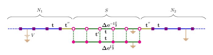
Figure 1: Schematic diagram of a superconducting ladder (S) connected to two normal metals ($N_{1}$,$N_{2}$). The left metal($N_{1}$) is maintained at a bias voltage $V$ while the superconducting ladder (S) and the right metal ($N_{2}$) are grounded. The intra-leg hopping of the Kitaev ladder and the hopping in the normal metals are $t$, the inter-leg ladder hopping is $t^{\prime}$ with chemical potential $\mu$ in all three regions. There is a superconducting pairing term $\Delta$ in each leg of the ladder with opposite superconducting phase factors ($\mp\frac{\phi}{2}$). The normal metals are connected to the upper leg of the ladder with a hopping $t^{\prime\prime}$.

The organization of our paper is as follows. The next section starts with a description of the model Hamiltonian and proceeds to a discussion of subgap Andreev states. The following section is about the boundary conditions, wavefunctions, scattering amplitudes and the calculation of transconductance. A Results and Analysis section puts together all the findings. The following section explores potential experimental realization of some of these phenomena. This is followed by a concluding summary section.

II Model Hamiltonian

The system under study consists of two normal metal leads coupled to a superconducting ladder as shown in Fig. 1. The superconducting ladder is made out of two Kitaev chains maintained at a phase difference of $\phi$. The first chain has the superconducting pair potential $\Delta e^{-i\phi/2}$, while the second chain has $\Delta e^{+i\phi/2}$. The two chains are connected by a hopping $t^{\prime}$ at each site as shown. The hopping in normal metal leads and the two Kitaev chains is $t$. The normal metal leads are connected to the upper Kitaev chain by a hopping $t^{\prime\prime}$.

The Hamiltonian for the metallic regions is given by

$$H_{N_{1}}=-t\displaystyle\sum_{n\leq-1}(c_{n+1}^{\dagger}c_{n}+c_{n}^{\dagger}c_{n+1})-\mu\displaystyle\sum_{n\leq 0}c_{n}^{\dagger}c_{n}$$ (1)

$$H_{N_{2}}=-t\displaystyle\sum_{n\geq L+1}(c_{n+1}^{\dagger}c_{n}+c_{n}^{\dagger}c_{n+1})-\mu\displaystyle\sum_{n\geq L+1}c_{n}^{\dagger}c_{n},$$ (2)

where $t$ is the hopping amplitude, the $c^{\dagger}_{n}(c_{n})$ are creation (annihilation) operators on the normal metals ($N_{1}$ for $n\leq 0$ or $N_{2}$ for $n\geq L+1$) and $\mu$ is the chemical potential. The dispersion in the normal metallic regions is the standard $E=\mp(2t\cos{ka}+\mu)$, where $-$ ($+$) sign corresponds to electrons (holes). The Hamiltonian for the Kitaev ladder is given by

$$H_{S}= \displaystyle\sum_{1\leq n\leq L-1\atop\sigma=1,2}-[(tc_{n+1,\sigma}^{\dagger}c_{n,\sigma}+\Delta e^{i\phi_{\sigma}}c_{n+1,\sigma}^{\dagger}c_{n,\sigma}^{\dagger})+h.c.]$$

$$-\displaystyle\sum_{1\leq n\leq L\atop\sigma=1,2}\mu c_{n,\sigma}^{\dagger}c_{n,\sigma}-t^{\prime}\displaystyle\sum_{1\leq n\leq L}[c_{n,1}^{\dagger}c_{n,2}+h.c.],$$ (3)

where $c^{\dagger}_{n,\sigma}$($c_{n,\sigma}$) are creation (annihilation) operators on the ladder ($1\leq n\leq L$) with $\sigma=1,2$ labeling the two legs. The hopping amplitude in each Kitaev chain is $t$. The inter-leg hopping in the superconducting ladder (S) is $t^{\prime}$ and the nearest-neighbor pairing with phase factor included is $\Delta e^{i\phi_{\sigma}}$ (in leg $\sigma$ of the ladder) with $\phi_{\sigma}=(-1)^{\sigma}\phi/2$. The full Hamiltonian is given by

$$H=H_{N_{1}}+H_{N_{1}S}+H_{S}+H_{N_{2}S}+H_{N_{2}},$$ (4)

where

$$H_{N_{1}S}=-t^{\prime\prime}[c_{0}^{\dagger}c_{1,1}+h.c.]$$ (5)

and

$$H_{N_{2}S}=-t^{\prime\prime}[c_{L+1}^{\dagger}c_{L,1}+h.c.]$$ (6)

are the terms that couple the superconducting ladder to the metallic leads at the two ends with hopping strength $t^{\prime\prime}$.

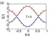
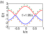
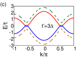
Figure 2: The dispersion of Kitaev ladder with $\phi=\pi$, $\Delta=0.1t$, $\mu=0.5t$. The inter-legs hoppings are (a)$t^{\prime}=\Delta$, (b)$t^{\prime}=1.95\Delta$, and (c)$t^{\prime}=3\Delta$. Two bands cross at $t^{\prime}=1.95\Delta$ for this value $\mu$ (Eq. 8). The solid curves correspond to $\nu_{2}=-1$ in Eq. (7) while the dashed curves correspond to $\nu_{2}=+1$.

The dispersion in the ladder region is

$$E=\nu_{1}\sqrt{\epsilon_{k}^{2}+{t^{\prime}}^{2}+\alpha_{k}^{2}+\nu_{2}\cdot 2t^{\prime}\sqrt{\epsilon_{k}^{2}+\alpha_{k}^{2}\leavevmode\nobreak\ \sin^{2}\frac{\phi}{2}}},$$ (7)

where $\nu_{1},\nu_{2}=\pm 1$ correspond to bands formed due to the hybridization of electron and hole excitations in the two legs of the ladder, $\phi=(\phi_{2}-\phi_{1})$, $\epsilon_{k}=-(2t\cos{ka}+\mu)$ and $\alpha_{k}=2\Delta\sin{ka}$. The dispersion here looks almost identical to the one for the $s$-wave superconducting ladder Soori and Mukerjee (2017), except for the appearance of the $k$-dependent part within $\alpha_{k}$. This spectrum yields four energy bands as can be seen in Fig. 2 for $\mu=0.5t$. The multiplicity of two for these bands corresponds to bonding and anti-bonding states formed by the hybridization of the two legs of the Kitaev ladder while another factor of two corresponds to Bogoliubov-de Genne (BdG) quasi-particles formed by the hybridization of electron and hole bands.

The energy spectrum shows that the gap closes for $t^{\prime}\geq 1.95\Delta$ for $\phi=\pi$ and $\mu=0.5t$. For a ladder with $\phi=\pi$, there exist plane wave BdG states at all energies within the superconducting gap when $t^{\prime}\geq 1.95\Delta$. Since the overall gap in the Kitaev ladder has $k$-dependence (Eq. 7), varying $\mu$ shifts the gap-closing point, in contrast to the s-wave model Soori and Mukerjee (2017). This motivates the computation of the energy gap of the ladder as a function of other parameters of the ladder Hamiltonian. Analytically, it can be shown from Eq. (7) that the gap closes only when $\phi=\pi$ and for:

$$t^{\prime}\geq\Delta\sqrt{4-\frac{\mu^{2}}{t^{2}-\Delta^{2}}}\leavevmode\nobreak\ .$$ (8)

The strongest lower bound here is seen to be $2\Delta$ corresponding to $\mu=0$.

When the two Kitaev chains are uncoupled, the spectrum has a gap, whose maximum value is $4\Delta$ (when the minimum of upper band is at $+2\Delta$ the maximum of the lower band is at $-2\Delta$). In the presence of a non-zero phase difference between the legs, as soon as the inter-leg coupling $t^{\prime}$ is turned on, plane wave states begin to appear inside this gap. Such states have a crucial role to play in the transport properties of the system, and are called subgap Andreev states. For small inter-leg couplings, despite the presence of subgap Andreev states, the ladder system still has a gap, although much lower. In order to quantify this, it is useful to study the logarithm of ‘the gap divided by $4\Delta$’ as shown in Fig. 3 (a) for $\mu=0.5t$ and $\Delta=0.1t$. It can be seen that the gap closes for $\phi=\pi$ and $t^{\prime}\geq 1.95\Delta$ - the closure of the gap provides further enhancement of transport, as will be described later. In Fig. 3 (b), the gap is plotted as a function of $\mu$ and $t^{\prime}$ for $\phi=\pi$ and $\Delta=0.1t$. The dark line in the plot indicates the value of $t^{\prime}$ above which the gap closes. It can be seen that the gap closes above a critical value of $t^{\prime}$ which depends on $\mu$ (Eq. (8)).

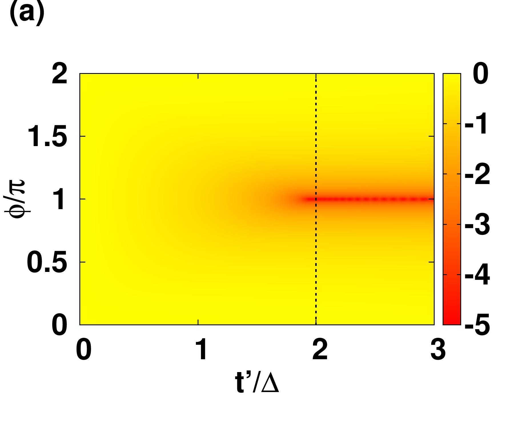
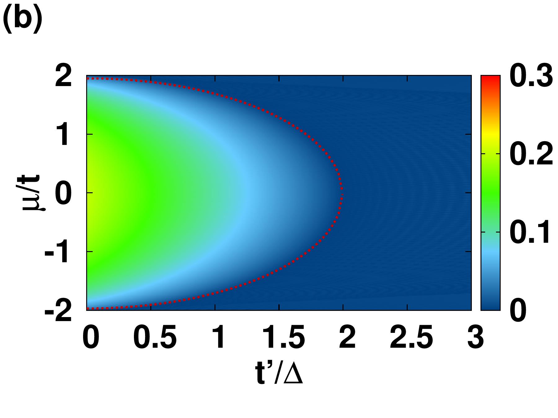
Figure 3: (a) Logarithm of ‘the energy gap divided by $4\Delta$’ for the ladder with parameters $\Delta/t=0.1$, $\mu/t=0.5$. The dotted line corresponds to $t^{\prime}/\Delta=2$, which is the strongest bound that can be realized when $\mu=0$ (Eq. (8)). (b) The energy gap for the parameters $\Delta/t=0.1$, $\phi=\pi$. The dark line separates gapless and gapped regions.

III Wave-functions and Transconductance

The wavefunction in the metallic regions has the form $[\psi_{e},\psi_{h}]^{T}$ and in the ladder region it has the form $\Psi=[\psi,\chi]^{T}$ where $\psi$ and $\chi$ both are two-spinors corresponding to the upper and the lower legs of the ladder respectively. For an electron incident from $N_{1}$ on to the ladder with an energy $E$, the wavefunction takes the following form in the metallic leads:

$$\psi_{n,e}=\begin{cases}\;e^{ik_{e}an}+r_{e}e^{-ik_{e}an}&{\rm for\leavevmode\nobreak\ \leavevmode\nobreak\ }n\leq 0,\\ \;t_{e}e^{ik_{e}an}&{\rm for\leavevmode\nobreak\ \leavevmode\nobreak\ }n\geq L+1,\end{cases}$$ (9)

$$\psi_{n,h}=\begin{cases}\;r_{h}e^{ik_{h}an}&{\rm for\leavevmode\nobreak\ \leavevmode\nobreak\ }n\leq 0,\\ \;t_{h}e^{-ik_{h}an}&{\rm for\leavevmode\nobreak\ \leavevmode\nobreak\ }n\geq L+1,\end{cases}$$ (10)

where $k_{e/h}a=\cos^{-1}\big{(}\frac{E\pm\mu}{2t}\big{)}$ and $r_{e}$, $r_{h}$, $t_{e}$, $t_{h}$ are the amplitudes for electron reflection, Andreev reflection, electron tunneling and cross Andreev reflection respectively. Here, $a$ is the lattice constant and $\hbar k_{e/h}$ is the electron/hole momentum. The wavefunction in the ladder region takes the form:

$$\psi_{n}=\displaystyle\sum_{\lambda,\nu,p}C_{\lambda,\nu,p}e^{i\lambda k_{\nu,p}an}[\psi_{e,\lambda,\nu,p}\leavevmode\nobreak\ ,\leavevmode\nobreak\ \psi_{h,\lambda,\nu,p}],$$ (11)

$$\chi_{n}=\displaystyle\sum_{\lambda,\nu,p}C_{\lambda,\nu,p}e^{i\lambda k_{\nu,p}an}[\chi_{e,\lambda,\nu,p},\chi_{h,\lambda,\nu,p}]$$ (12)

for $1\leq n\leq L$, where $\lambda=\pm 1$ refers to forward/backward motion of BdG quasiparticles, $\nu=\pm 1$ refer to anti-bonding/bonding bands and $p=\pm 1$ refers to electronlike/holelike bands. At a given energy $E$, $k_{\nu,p}a$ is found by numerically solving the quartic equation for $\cos{k_{\nu,p}a}$ which is obtained by manipulating Eq. (7), and the spinor $[\psi_{e,\lambda,\nu,p},\leavevmode\nobreak\ \psi_{h,\lambda,\nu,p},\leavevmode\nobreak\ \chi_{e,\lambda,\nu,p},\leavevmode\nobreak\ \chi_{h,\lambda,\nu,p}]^{T}$ is the eigenspinor of the ladder Hamiltonian in momentum space with energy $E$ and momentum $\lambda\hbar k_{\nu,p}$. Here, the normal metal lead is connected by a hopping to the upper leg of the ladder (Fig 1). From the Hamiltonian (Eq. (4)) the equation of motion at each site on either side of the junction can be written down. There are six sites and two equations at each site due to particle-hole nature of the equations making it twelve equations totally which are just enough to solve for twelve scattering amplitudes in Eqs. (9), (10), (11), and  (12). The details of this calculation are shown in the Appendix.

A useful quantity to study the relative contribution of CAR with respect to ET is the differential transconductance. Also, this is the physical quantity that is measured in transport experiments. The ladder attached to two normal metals is biased so that a voltage $V$ is applied to $N_{1}$ keeping the ladder and $N_{2}$ grounded. The differential transconductance, $G_{21}:=\frac{dI_{2}}{dV_{1}}$ is the ratio of change in the current $dI_{2}$ in $N_{2}$ to the change in the applied voltage $dV_{1}$ in $N_{1}$. From Landauer-Büttiker formalism Landauer (1957, 1970); Büttiker et al. (1985); Büttiker (1986); Datta (1995), the differential transconductance of the system at bias $V_{1}$ is given by

$$G_{21}=\frac{e^{2}}{h}\Bigg{(}|t_{e}|^{2}-|t_{h}|^{2}\frac{\sin{k_{h}a}}{\sin{k_{e}a}}\Bigg{)}.$$ (13)

Here, the first term represents the contribution to transconductance from ET while the second term represents the contribution due to CAR. Therefore, a positive $G_{21}$ is a clear signature of enhanced ET while a negative $G_{21}$ is a signature of enhanced CAR.

IV Results and analysis

IV.1 Variation of $\mu$

One special case where crossed Andreev reflection happens is when $\phi=0$. In this case, the two legs of the ladder retain their Majorana fermions and crossed Andreev reflection can happen by the non-local state formed by the coupling between two Majorana bound states at the end. But this carries no net current due to the competing electron tunneling which has a magnitude of current that is same as that of crossed Andreev reflection Nilsson et al. (2008). In general, we find that choosing $\phi=\pi$ and $t^{\prime\prime}=t$ works best for the enhancement of CAR and ET, and therefore fix $\phi=\pi$ and $t^{\prime\prime}=t$ in this paper, unless specified otherwise.

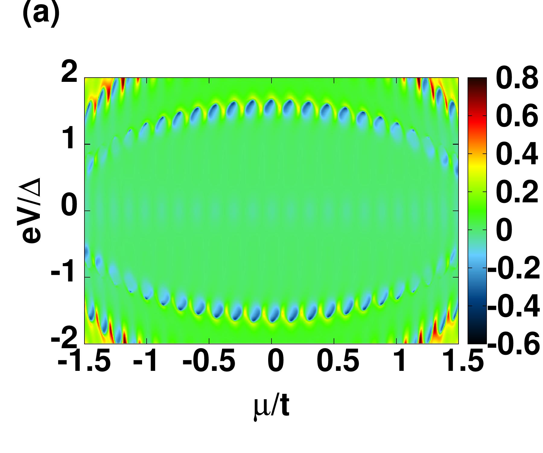
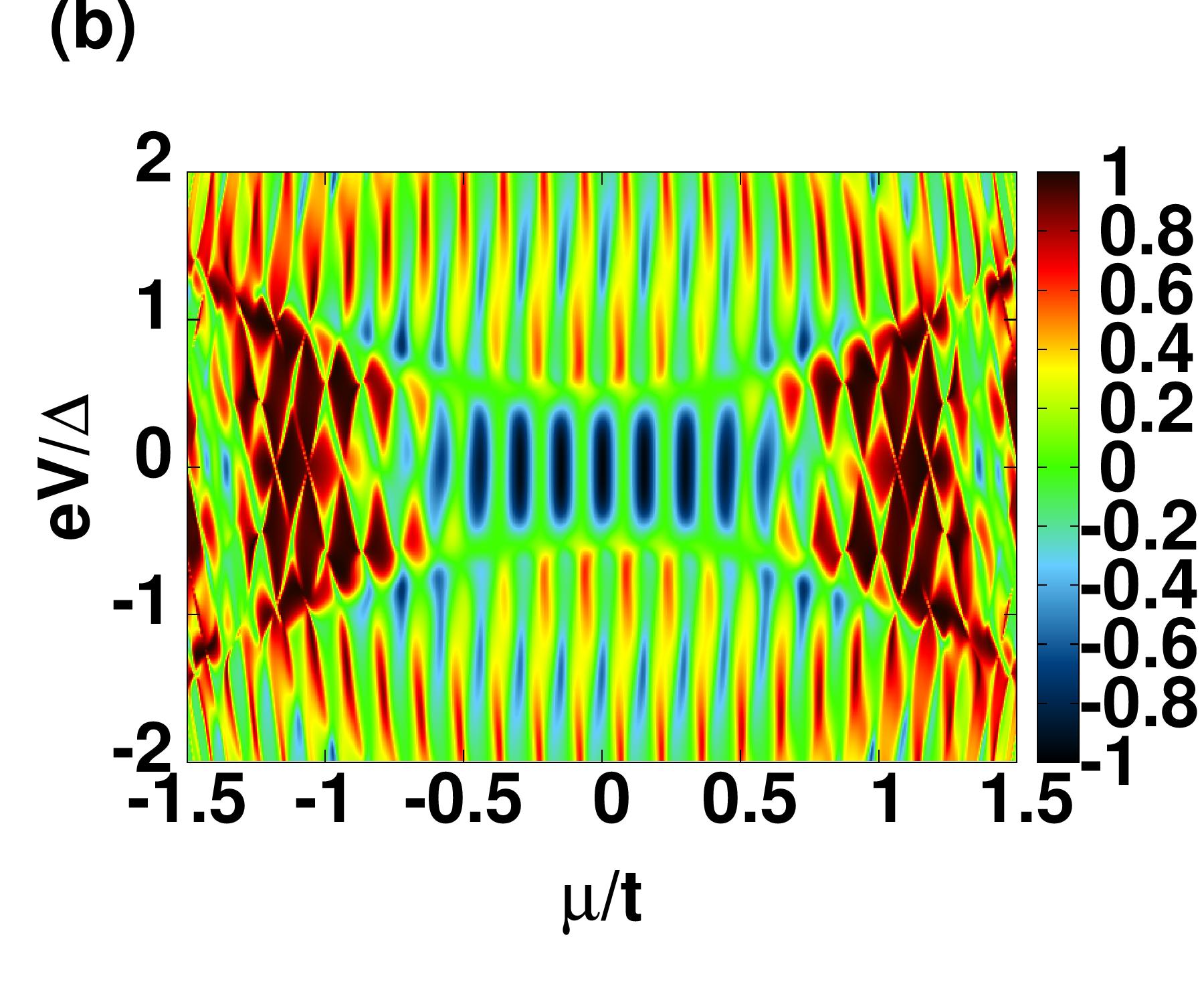
Figure 4: The transconductance $G_{21}$ in units of $e^{2}/h$ for the parameters: $\Delta=0.1t$, $t^{\prime\prime}=t$, $\phi=\pi$, $L=40$ and (a) $t^{\prime}=\Delta$ (b) $t^{\prime}=3\Delta$. (a) Below the critical value of inter-leg hopping, the transconductance is mainly zero while (b) beyond the critical value an enhancement of both CAR and ET can be seen due to the presence of subgap Andreev states.

In Fig. 4 we plot the differential transconductance as a function of bias and chemical potential for two values of the inter-leg hoppings: (a) $t^{\prime}=\Delta$ and (b) $t^{\prime}=3\Delta$. We see that the transconductance is mostly suppressed for the case $t^{\prime}<2\Delta$, while for the case $t^{\prime}>2\Delta$, one can find thick regions in the plot where the transconductance is enhanced. Enhancement of differential transconductance in magnitude is due to the existence of subgap Andreev states.

Some of the results in Fig. 4 are replotted in Fig. 5 for clarity.

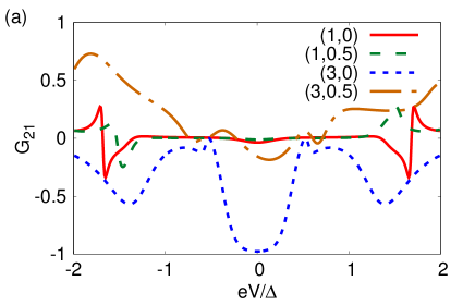
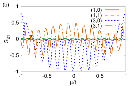
Figure 5: The transconductance $G_{21}$ in units of $e^{2}/h$ as a function of (a) bias voltage and (b) chemical potential (some of the results in Fig. 4 plotted as line plot). The legend shows (a) $(t^{\prime}/\Delta,\mu/t)$, (b) $(t^{\prime}/\Delta,eV/\Delta)$ for different curves.

It can be seen from both the plots that the magnitude of transconductance is high for $t^{\prime}=3\Delta$. In Fig. 5(a), it can be seen that $G_{21}$ is not a symmetric function of $eV$ for $\mu=0.5t$, while $G_{21}$ is a symmetric function of $eV$ for $\mu=0$. In Fig. 5(b), one can see periodic oscillations of transconductance as a function of $\mu$, which we will soon touch upon.

Before we analyze the origin of enhanced CAR and ET, let us examine the contribution of various processes in the transport. An incident electron can do one of four things: reflect back (ER -electron reflection), reflect back as a hole (AR -Andreev reflection), transmit through and emerge out as electron (ET -electron tunneling) or transmit through and emerge out as a hole (CAR -crossed Andreev reflection). Conservation of probability currents for these processes implies Blonder et al. (1982); Soori et al. (2013)

$$|r_{e}|^{2}+|t_{e}|^{2}+(|r_{h}|^{2}+|t_{h}|^{2})\frac{\sin{k_{h}a}}{\sin{k_{e}a}}=1.$$ (14)

We now examine these components for the set of parameters as in Fig. 4(a) and 4(b).

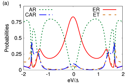
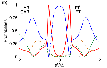
Figure 6: The probability of four processes as shown in Eq. (14) as a function of applied bias for parameters (a)$t^{\prime}=\Delta$, (b) $t^{\prime}=3\Delta$ same as Fig. 4 and $\mu=0$. It can be seen that (a) below the critical value ER and AR dominates while (b) going beyond the critical value CAR and ER dominates with CAR touching its maximum value around the zero bias voltage.

It can be seen from Fig. 6(a) that when $t^{\prime}=\Delta$, ER and AR dominate the transport. It can be seen from Fig. 6(b) that when $t^{\prime}=3\Delta$, CAR dominates the transport around zero bias. This feature is one of the unique aspects of the present setup. Such CAR-enhanced regions can also be seen in the contour plot of Fig. 4(b) where $G_{21}$ hits values close to $-e^{2}/h$. We now turn to the dependence of various probabilities on $\mu$ in the zero bias case.

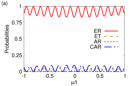
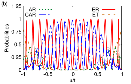
Figure 7: The probability of various processes in system as a function of chemical potential for (a) $t^{\prime}=\Delta$ and (b) $t^{\prime}=3\Delta$ with other parameter same as Fig. 4 and $eV=0$. Here, CAR dominates over other processes after crossing of bands when $t^{\prime}\geq 2\Delta$.

From Fig. 7(a), we can see that for $t^{\prime}=\Delta$, ER dominates and the other three process are suppressed at zero bias. From Fig. 7(b), we can see that for $t^{\prime}=3\Delta$, ER and CAR are enhanced. Whether ER is enhanced or CAR is enhanced depends on the exact value of $\mu$ and one is enhanced at the expense of the other while suppressing ET and AR. In non-local conductance measurements, only $G_{21}$ which is a linear combination of CAR and ET probabilities can be measured; the two probabilities cannot be separately measured.

In Fig. 8, we plot the subgap energy states of the isolated ladder as a function of $\mu$ for the same parameters as in Fig. 4. The features in Fig. 4 can be directly compared with Fig. 8.

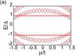
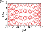
Figure 8: The energy spectrum of the isolated Kitaev ladder with open boundary conditions for (a) $t^{\prime}=\Delta$, (b) $t^{\prime}=3\Delta$ such that the other parameters are $\Delta=0.1t$, $\phi=\pi$, $L=40$. The gapped region in (a) shows the sparsely spaced subgap Andreev states whereas going beyond a critical value of inter-leg hopping these states become dense (b).

We can see a resemblance between the features of the two plots in Fig. 4 and the features of the plots for respective parameters in Fig. 8. The resemblance is a signature of resonant transmission of charge from one reservoir to another through a quantum dot where the ladder plays the role of the quantum dot Roy et al. (2009); Soori (2019).

In Fig. 4(a) (for $t^{\prime}<2\Delta$), the center of the bias window has zero transconductance, since there are no states available in this region as confirmed in Fig. 8(a). On the other hand, there is high ET and CAR near the boundary of the window; correspondingly the presence of energy levels in that region is shown in Fig. 8(a). In Fig. 4(b) (for $t^{\prime}>2\Delta$) the CAR and ET both show enhancement due to the presence of subgap states as shown in Fig. 8(b). These subgap states provide the plane wave modes which promote the transmission of quasiparticles. It is seen from Fig. 4(b) that both ET and CAR show periodic behavior with varying chemical potential ($\mu$). This periodicity in differential transconductance can be understood as due to Fabry-Pérot interference of subgap Andreev states in the ladder region. The Fabry-Pérot interference condition $(k_{i+1}-k_{i})aL\approx\pi$ gives a spacing of $\delta\mu\approx 0.157t$ between consecutive peaks in transconductance values for the parameters of Fig. 4(b) in the region $eV=0$ and $\mu\approx 0$. This agrees with the spacing in the transconductance plot of Fig. 4(b).

Figure 9: The transconductance $G_{21}$ (in units of $e^{2}/h$) for the same parameters as in Fig. 4 but with a smaller system size ($L=10$). The smaller system size allows for the electrons (holes) to tunnel through the junction even though the inter-leg hopping is below the critical value (a), whereas for the choice of $t^{\prime}$ above the critical value the enhancement of CAR and ET to its extreme value is obtained (b). The parameters are: $\Delta=0.1t$, $\mu=0.5t$, $\phi=\pi$ and (a) $t^{\prime}=\Delta$ (b) $t^{\prime}=3\Delta$.

However, for very small system sizes the transconductance shows distinctly different behavior as can be seen in Fig. 9, which is the same as Fig. 4 but with $L=10$. For $t^{\prime}=\Delta$, the ET is enhanced with a maximum conductance of $0.8e^{2}/h$ whereas for $t^{\prime}=3\Delta$ the CAR dominates with an extremum value of $-e^{2}/h$ along with enhanced ET mainly at the corners of the contour plot with a maximum value of $e^{2}/h$.

IV.2 Variation of $L$

The different behavior of transconductance for two different lengths of the Kitaev ladder motivates a systematic study of its variation with system size shown in Fig. 10 and Fig. 11. Fig. 10(a) or the dashed line in Fig. 11 reveal that for $t^{\prime}<2\Delta$, the zero transconductance region is dominant unless the system size is below a characteristic length scale. The initial red region in Fig. 10(a) characterizes ET due to presence of the decaying modes where the ladder length is so small that an electron can tunnel through the ladder. This is a reflection of change of the nature of transport Tan et al. (2015); Sadovskyy et al. (2015) from ballistic to diffusive as the length is increased.

Figure 10: The system size variation of transconductance (plotted in units of $e^{2}/h$) in the two regimes: (a) below the critical value of inter-leg hopping ($t^{\prime}=\Delta$) and (b) above the critical value $t^{\prime}=3\Delta$. The decaying modes in (a) suppress transport for larger system sizes for $eV<|\Delta|$, however for $eV>|\Delta|$ the plane wave BdG modes are responsible for the transport. The periodic nature in (b) appears as a consequence of Fabry-Pérot resonance. The other parameters are: $\Delta=0.1t$, $\mu=0.5t$, $\phi=\pi$.

For $t^{\prime}>2\Delta$ oscillatory behavior kicks in as a result of the Fabry-Pérot resonance phenomenon described earlier. Therefore as shown in Fig. 10(b) and dotted lines in Fig. 11, both ET and CAR are enhanced periodically.

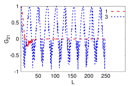
Figure 11: The zero bias transconductance as a function of length for the same choice of parameters as in Fig. 10 with the different values of $t^{\prime}/\Delta$ shows the oscillatory behavior for $t^{\prime}>2\Delta$ .

The region $|eV|<\Delta$ corresponds to all eight $k$’s being real while the region $|eV|>\Delta$ corresponds to only four $k$’s being real-valued while the other four $k$’s complex valued. Thus, there are less modes leading to interference in the region $|eV|>\Delta$ compared to the region $|eV|<\Delta$ and this reflects in the richer interference pattern in the latter region.

IV.3 Variation of $t^{\prime}$, $t^{\prime\prime}$ and $\phi$

Features of the transconductance plot as a function of bias $eV$ and the inter-leg hopping $t^{\prime}$ are presented in Fig. 12(a). At zero bias, for $t^{\prime}\leq 2\Delta$, the transconductance is suppressed while for $t^{\prime}\geq 2\Delta$, the transconductance is enhanced periodically. At nonzero bias, there are three regions- the region where the transconductance is highly suppressed, the region where the transconductance is moderately enhanced and is periodic and the third region where the transconductance is highly enhanced and periodic. These regions respectively correspond to all eight momenta in the ladder region imaginary, only four momenta in the ladder region real and all eight momenta in the ladder region real respectively.

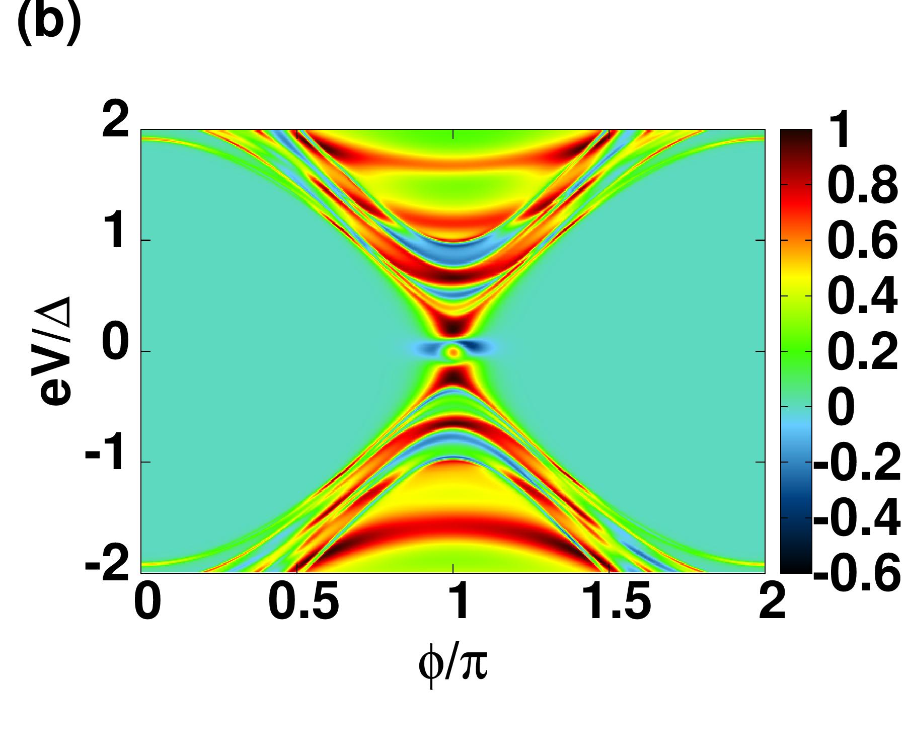
Figure 12: The transconductance $G_{21}$ in units of $e^{2}/h$ as a function of bias and: (a) inter-leg hopping of the ladder for $\phi=\pi$, (b) phase difference for $t^{\prime}=3\Delta$. The band crossing after a critical value of inter-leg hopping provides the propagating modes (a) and the enhancement is more prominent around $\phi\approx\pi$ (b). Parameters common to (a) and (b): $\Delta=0.1t$, $t^{\prime\prime}=t$, $\mu=0.50$, and $L=100$.

A substantial superconducting phase difference between the two legs of the Kitaev ladder promotes enhanced transconductance. This can be seen in Fig 12(b) and Fig. 13.

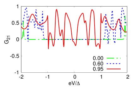
Figure 13: Transconductance in units of $e^{2}/h$ as a function of applied bias for the same choice of parameters as in Fig. 12(b) with different values of $\phi/\pi$.

Here, we have chosen the inter-leg hopping $t^{\prime}=3\Delta$ so that there are subgap Andreev states in the ladder for large phase difference $\phi$. For small values of the phase difference and values of the phase difference close to $2\pi$, the transconductance is suppressed. For values of the phase difference in the range $\pi/2\lesssim\phi\lesssim 3\pi/2$, we see a rich interference pattern where CAR and ET are enhanced in certain regions. This interference pattern has origins in the Fabry-Pérot interference of the subgap Andreev states.

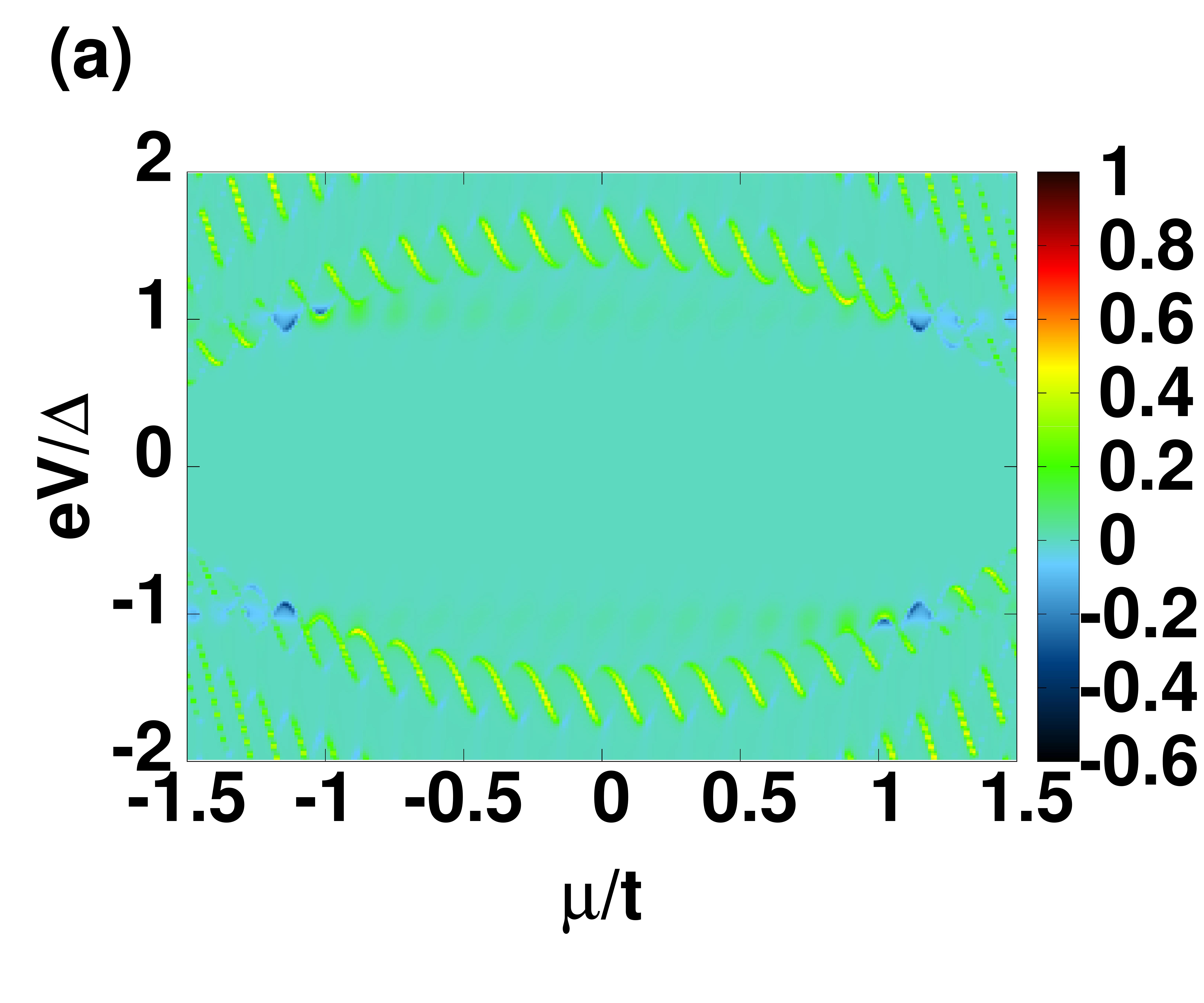
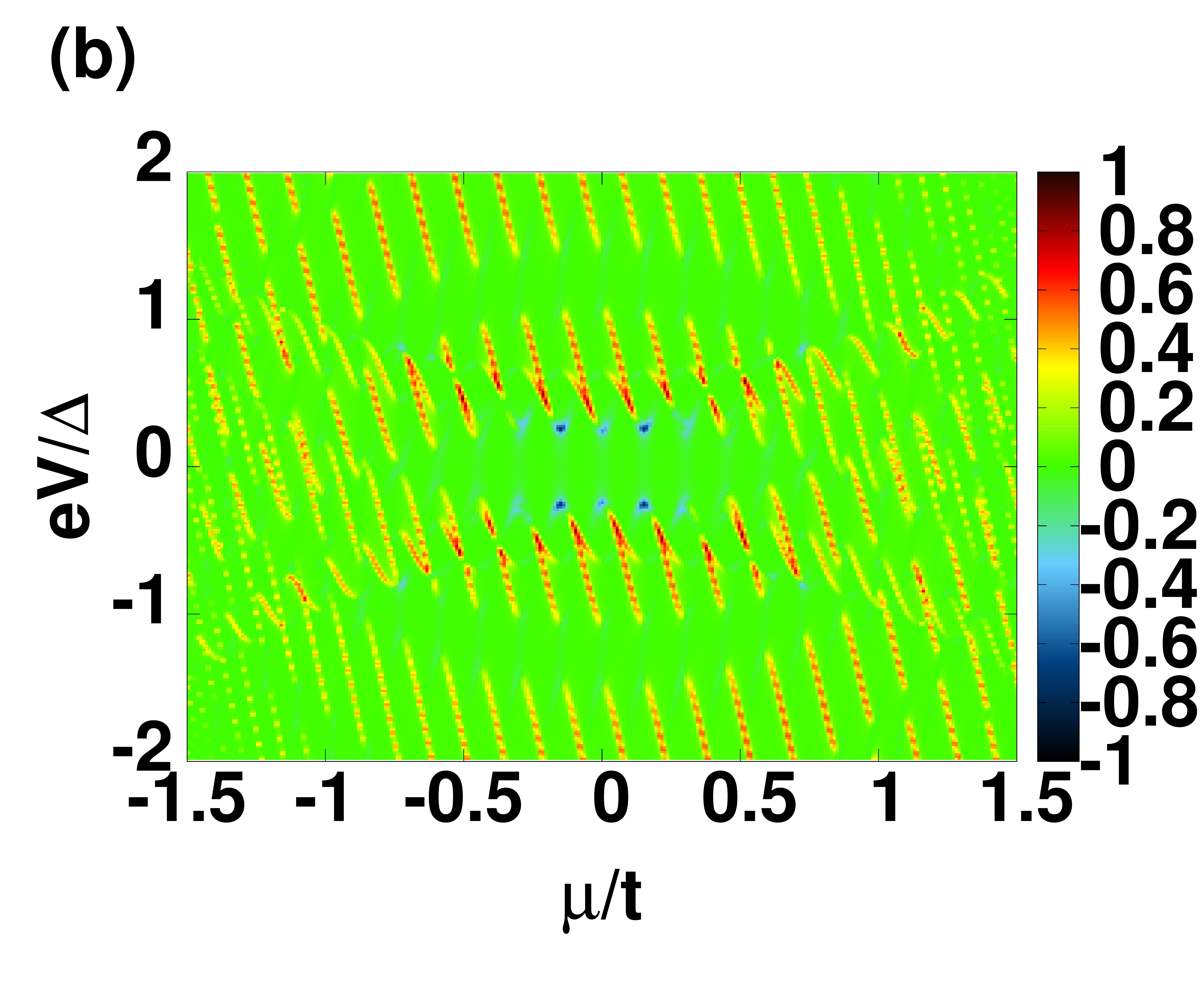
Figure 14: The transconductance $G_{21}$ in units of $e^{2}/h$ for the parameters: $\Delta=0.1t$, $t^{\prime\prime}=0.3t$, $\phi=\pi$, $L=40$ and (a) $t^{\prime}=\Delta$ (b) $t^{\prime}=3\Delta$. The suppression of transport in most regions compared to Fig. 4 can be seen .

We have studied a system where the junction is ideal and perfectly transmitting. In a realistic system, the junction may not be perfectly transmitting. Such a junction can be modeled by changing the hopping term from normal metal lead to the SC ladder away from hopping in the normal metal lead, that is $t^{\prime\prime}\neq t$. The ladder then is weakly connected to normal metal leads and transport happens only at bias energies equal to the energies of the isolated ladder hosting standing waves. The contour plot of the differential transconductance versus bias and chemical potential is expected to resemble more closely with Fig. 8. In Fig. 14, we plot a contour plot of the transconductance versus bias and chemical potential for the same choice of parameters as in Fig. 4, except that $t^{\prime\prime}=0.3t$ making the interface less transparent. This shows that it is important to have an interface which is as close to ideal as possible.

V Experimental Realization

In this Section, we include a brief discussion of the possibility of an experimental realization of the proposed setup. While a Kitaev chain hosting Majorana fermions at its ends is realized in semiconductor quantum wires Mourik et al. (2012); Albrecht et al. (2016), ladder systems have been discussed in recent literature Wakatsuki et al. (2014). Once two Kitaev chains are realized they can be separated by a thin gated insulator layer. The gate voltage can be used to tune the hopping between the two chains. A loop can be made between the superconductors proximetizing the two chains and a magnetic flux through such a loop can be used to control the superconducting phase difference as discussed in Ref. Keselman et al. (2013). Thus, a Kitaev ladder with controllable phase difference and hopping can be realized. We envisage that experimental groups will be motivated by our work to explore these directions further.

Once the ladder is realized, another way to probe nonlocal transport is to measure current-current correlations Nilsson et al. (2008). For this, both the normal metal leads are maintained at a bias $V$ and the ladder is grounded. Then equal amount of current flows in each of the leads. In this configuration, the current that flows in the leads has contributions from local Andreev reflection and nonlocal CAR. If $I_{1}(t)$ and $I_{2}(t)$ are currents at time $t$ in NM1 and NM2 respectively, the nonlocal noise power can be defined as $P_{12}=\int_{-\infty}^{\infty}dt\overline{\delta I_{1}(0)\delta I_{2}(t)}$ and the corresponding Fano factor is $F_{12}=P_{12}/e\bar{I_{1}}$, where $\bar{I_{i}}$ is time averaged current in lead $i$ and $\delta I_{i}(t)=I_{i}(t)-\bar{I_{i}}$ is the current fluctuation in lead $i$. A positive maximal value of $F_{12}=1$ corresponds to maximally enhanced CAR.

VI Summary

To summarize, we studied a ladder consisting of two Kitaev chains maintained at a superconducting phase difference and connected to leads at either ends. We see that a nonzero phase difference and a sufficiently large inter-leg hopping generates plane wave states within the superconducting gap of the isolated ladder. We call these subgap Andreev states. The gap of the spectrum closes for sufficiently large inter-leg hopping which depends on the choice of the chemical potential (for $\mu=0$, the gap closes when $t^{\prime}\geq 2\Delta$) and for the choice $\phi=\pi$. We showed that the subgap Andreev states are responsible for enhanced crossed Andreev reflection and enhanced electron tunneling. For a long ladder, one can see a resemblance in the energy spectrum of the isolated ladder and the differential transconductance indicating that the patterns in the differential transconductance are due to the resonant levels present in the ladder region. We studied the dependence of the transconductance on various parameters such as the bias, chemical potential, length of the ladder, inter-leg hopping strength and the phase difference. We find that by tuning the parameters, one can get values of negative transconductance with high magnitude which indicates enhanced crossed Andreev reflection. We find periodic patterns in transconductance when the subgap Andreev states exist in the ladder and the periodic patterns can be understood as originating from the Fabry-Pérot resonance between the plane wave modes in the ladder. We also show that it is important to have a transparent interface between the ladder and the leads to enhance crossed Andreev reflection.

Appendix A Equation of motion at the boundaries

In this appendix, we have given a detailed calculation of the various scattering amplitudes. The plane wave solution for electrons and holes in the metallic regions are :

$$\psi_{n,e}=\begin{cases}\;e^{ik_{e}an}+r_{e}e^{-ik_{e}an}&{\rm for\leavevmode\nobreak\ \leavevmode\nobreak\ }n\leq 0,\\ \;t_{e}e^{ik_{e}an}&{\rm for\leavevmode\nobreak\ \leavevmode\nobreak\ }n\geq L+1,\end{cases},\qquad\psi_{n,h}=\begin{cases}\;r_{h}e^{ik_{h}an}&{\rm for\leavevmode\nobreak\ \leavevmode\nobreak\ }n\leq 0,\\ \;t_{h}e^{-ik_{h}an}&{\rm for\leavevmode\nobreak\ \leavevmode\nobreak\ }n\geq L+1,\end{cases},$$ (15)

where, $r_{e}$, $r_{h}$ are reflection coefficients and $t_{e}$, $t_{h}$ are transmission coefficients of electrons and holes in the two metallic regions. Also, $k_{e}=\cos^{-1}\big{(}\frac{E+\mu}{2t}\big{)}$ and $k_{h}=\cos^{-1}\big{(}\frac{E-\mu}{2t}\big{)}$ are momenta of electron and hole respectively.

The wavefunction for the ladder system is given by

$$\psi_{n}=\displaystyle\sum_{\lambda,\nu,p}C_{\lambda,\nu,p}e^{i\lambda k_{\nu,p}an}[\psi_{e,\lambda,\nu,p}\leavevmode\nobreak\ ,\leavevmode\nobreak\ \psi_{h,\lambda,\nu,p}],$$ (16)

$$\chi_{n}=\displaystyle\sum_{\lambda,\nu,p}C_{\lambda,\nu,p}e^{i\lambda k_{\nu,p}an}[\chi_{e,\lambda,\nu,p},\chi_{h,\lambda,\nu,p}]$$ (17)

where, the different quantities are same as defined in the main text (Section III). For a given energy we have $8$ momenta values $\lambda k_{\nu,p}$’s (corresponding to $\pm$ values of the three variables $\lambda,\nu,p$) which can be numerically found from Eq. 7. Overall there are $12$ unknowns as can be seen from Eqs. 15, 16 and 17. These unknowns can be calculated by writing the equations of motion from the Hamiltonian (Eq. 4) at the two boundaries as shown in Fig 15.

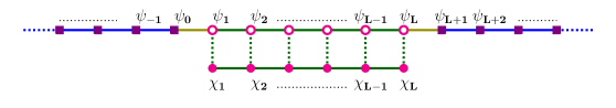
Figure 15: A schematic of the system delineating the wavefunctions at the different sites of the system.

These equations are:

$$E\psi_{0,e}=-t^{\prime\prime}\psi_{1,e}-t\psi_{-1,e}-\mu\psi_{0,e}$$ (18)

$$E\psi_{0,h}=t^{\prime\prime}\psi_{1,h}+t\psi_{-1,h}+\mu\psi_{0,h}$$ (19)

$$E\psi_{1,e}=-t\psi_{2,e}-t^{\prime\prime}\psi_{0,e}-\mu\psi_{1,e}-t^{\prime}\chi_{1,e}-\Delta e^{i\phi_{1}}\psi_{2,h}$$ (20)

$$E\psi_{1,h}=t\psi_{2,h}+t^{\prime\prime}\psi_{0,h}+\mu\psi_{1,h}+t^{\prime}\chi_{1,h}+\Delta e^{-i\phi_{1}}\psi_{2,e}$$ (21)

$$E\chi_{1,e}=-t\chi_{2,e}-\mu\chi_{1,e}-t^{\prime}\psi_{1,e}-\Delta e^{i\phi_{2}}\chi_{2,h}$$ (22)

$$E\chi_{1,h}=t\chi_{2,h}+\mu\chi_{1,h}+t^{\prime}\psi_{1,h}+\Delta e^{-i\phi_{2}}\chi_{2,e}$$ (23)

$$E\psi_{L+1,e}=-t\psi_{L+2,e}-t^{\prime\prime}\psi_{L,e}-\mu\psi_{L+1,e}$$ (24)

$$E\psi_{L+1,h}=t\psi_{L+2,h}+t^{\prime\prime}\psi_{L,h}+\mu\psi_{L+1,h}$$ (25)

$$E\psi_{L,e}=-t^{\prime\prime}\psi_{L+1,e}-t\psi_{L-1,e}-\mu\psi_{L,e}-t^{\prime}\chi_{L,e}+\Delta e^{i\phi_{1}}\psi_{L-1,h}$$ (26)

$$E\psi_{L,h}=t^{\prime\prime}\psi_{L+1,h}+t\psi_{L-1,h}+\mu\psi_{L,h}+t^{\prime}\chi_{L,h}-\Delta e^{-i\phi_{1}}\psi_{L-1,e}$$ (27)

$$E\chi_{L,e}=-t\chi_{L-1,e}-\mu\chi_{L,e}-t^{\prime}\psi_{L,e}+\Delta e^{i\phi_{2}}\chi_{L-1,h}$$ (28)

$$E\chi_{L,h}=t\chi_{L-1,h}+\mu\chi_{L,h}+t^{\prime}\psi_{L,h}-\Delta e^{-i\phi_{2}}\chi_{L-1,e}.$$ (29)

Finally, the various unknowns can be calculated by solving these equations. The transconductance can be then calculated from Eq. 13.