Abstract

Latent force models are a class of hybrid models for dynamic systems, combining simple mechanistic models with flexible Gaussian process (GP) perturbations. An extension of this framework to include multiplicative interactions between the state and GP terms allows strong a priori control of the model geometry at the expense of tractable inference.

In this paper we consider two methods of carrying out inference within this broader class of models. The first is based on an adaptive gradient matching approximation, and the second is constructed around mixtures of local approximations to the solution. We compare the performance of both methods on simulated data, and also demonstrate an application of the multiplicative latent force model on motion capture data.

1 Introduction

Historically the modelling of dynamic systems broadly followed one of two distinct philosophies; the first of these is classical and often referred to as the mechanistic approach which aims to construct realistic models guided by sound principles. In contrast, the data driven paradigm, inspired by modern machine learning techniques, places a greater emphasis on prediction, and allowing the observables to guide the processes of pattern discovery. The conflict between these two philosophies can be particularly pronounced for complex dynamic systems, when a complete mechanistic description is often difficult to motivate, but models with some degree of physical realism are likely to be more effective extrapolating from the training data. Therefore, it would be desirable to have a framework that allows for the specification of a simplistic representation of the driving dynamics, while still allowing for relevant dynamic systems properties to be encoded into the model. One successful approach to constructing such hybrid models is the latent force model (LFM) introduced in [Alvarez et al., 2009]. By combining a simple class of mechanistic models with the flexibility offered by inhomogenous Gaussian process (GP) pertubations one is able to construct a GP regression, with dynamic systems properties encoded within the kernel function.

While the GP regression framework allows for tractable inference this assumption is also one of the primary constraints of the LFM. In an effort to move beyond this constraint [Tait and Worton, 2018] introduced an extension of this model, while staying faithful to the underlying modelling framework; a linear time dependent ordinary differential equation (ODE) in which the time dependent behaviour arises from the variations of a set of independent GP variables, but now allowing multiplicative interactions between the state and latent forces. The result is a semi-parametric model that allows for the embedding of rich topological structure.

Unfortunately, the greater control of the model geometry comes at the expense of the tractable GP regression framework of the LFM, and therefore we must necessarily consider approximate inference methods. In this paper we consider two methods of introducing approximate likelihood functions for this class of models. The first is an application of adaptive gradient matching methods introduced by [Calderhead et al., 2009, Dondelinger et al., 2013] for handling problems in the very general class of nonlinear ODEs with random parameters. The second combines truncated local approximations to the pathwise solution of the ODE using a mixture modelling approach.

In the next section we provide a review of the LFM framework, including the extension allowing for multiplicative interactions. Then in Section 3 we discuss how the adaptive gradient matching methods can be used to introduce an approximate inference method for the extended of the latent force model, and demonstrate they lead to a practical simplification in the linear case. We then consider the method based on local successive approximations in Section 4. In Section 5 we compare the performance of the two methods on simulated data, and in Section 6 we demonstrate the viability of the model with multiplicative interactions with an application to the modelling of human motion capture data using geometry constrained models before concluding with a discussion.

2 LATENT FORCE MODELS

Latent force models [Alvarez et al., 2009] are a class of hybrid models of dynamic systems providing a compromise between purely data driven approaches, and more involved mechanistic models. They combine the simplest class of mechanistic models; linear ODEs with, diagonal, constant coefficient matrices with the flexibility of an additive GP forcing term. In what follows we let $\mathbf{x}(t)$ denote a $K$-dimensional state variable, and we collect $R$ independent, smooth, GPs into a vector valued process $\mathbf{g}(t)=(g_{1}(t),\ldots,g_{R}(t))^{\top}$. Then the LFM is described by the initial value problem (IVP)

$$\frac{\mathrm{d}\mathbf{x}(t)}{\mathrm{d}t}=\mathbf{D}\mathbf{x}(t)+\mathbf{S}\mathbf{g}(t),$$ (1)

where $\mathbf{D}$ is a diagonal matrix, and the sensitivity matrix, $\mathbf{S}$, is a $K\times R$ real valued rectangular matrix. From (1) it is clear that the only interactions between the state variables, $x_{k}(t)$, is through the common latent force variables, and the sensitivity matrix governs the topology of these interactions. The LFM encodes dynamic systems properties, but still allows for tractable inference because the solution may be expressed as a linear transformation of the latent GPs

$$\mathbf{x}(t)=e^{\mathbf{D}(t-t_{0})}\mathbf{x}(t_{0})+e^{\mathbf{D}t}\int_{t_{0}}^{t}e^{-\tau\mathbf{D}t}\mathbf{S}\mathbf{g}(\tau)\mathrm{d}\tau,$$ (2)

this linear relationship between the states and latent GPs results in a joint Gaussian distribution. This property makes it possible to marginalise over the latent forces, so that inference for the LFM may proceed exactly as in standard GP regression.

The GP regression framework leads to straightforward inference, but the assumption of Gaussian trajectories of the state variable may be implausible; this will be the case for time series of circular, directional data, and tensor valued data. With this in mind [Tait and Worton, 2018] proposed an extension of the LFM retaining the linear ODE framework, but allowing for non-Gaussian trajectories by including multiplicative interactions between the GP forcing functions and the state variables which they refer to as the multiplicative latent force model (MLFM).

The MLFM may be represented by the linear ODE

$$\frac{\mathrm{d}\mathbf{x}(t)}{\mathrm{d}t}=\mathbf{A}(t)\mathbf{x}(t),\qquad\mathbf{A}(t)=\mathbf{A}_{0}+\sum_{r=1}^{R}\mathbf{A}_{r}\cdot g_{r}(t).$$ (3)

The dynamics will be governed by the support of the $K\times K$ coefficient matrix $\mathbf{A}(t)$, which by linearity will be a matrix valued GP interacting multiplicatively with the state variable, the support of this GP will be determined by the coefficient matrices $\mathbf{A}_{r}$.

To add further flexibility we allow each of the structure matrices, $\mathbf{A}_{r},r=0,1,\ldots,R$ to be given as a linear combination of a set of shared basis matrices $\mathbf{L}_{d}$, $d=1,\ldots,D$, that is

$$\mathbf{A}_{r}=\sum_{d=1}^{D}\beta_{rd}\mathbf{L}_{d}.$$ (4)

We denote the set of connection coefficients by the $(R+1)\times D$ matrix $\mathbf{B}$ with $\mathbf{B}_{rd}=\beta_{rd}$. Including these variables allows a small set of forces to generate a broad range of motions, and they play a role analogous to the sensitivity matrix in (1). As is common in many modern machine learning techniques this increase in flexibility, and predictive power, comes at the expense of identifiability of individual parameters.

The multiplicative interactions in (3) and the freedom to chose the support of the coefficient matrices enables the modeller to embed strong geometric constraints into the pathwise solution of this model. Noteworthy is the case when the elements $\{\mathbf{L}_{d}\}_{d=1}^{D}$ are members of a Lie algebra $\mathfrak{g}$ with corresponding matrix Lie group $G$, [Hall, 2015]. Since $\mathfrak{g}$ is a vector space the support of $\mathbf{A}(t)$ will be contained within this Lie algebra. It follows from this constraint that the fundamental solution of (3) will itself be a member of the Lie group $G$, [Iserles and Nørsett, 1999], therefore allowing the construction of models either on this group, or formed by the action of random elements within this group on some vector space. This possibility to embed strong geometric constraints within the model is the primary motivation for introducing this extension of the LFM.

The remarks on the geometry preservation above combined with the flexibility of choosing the support of $\mathbf{A}(t)$ via the choice of the basis matrices $\{\mathbf{L}_{d}\}$ and their connection coefficients $\mathbf{B}$ allow the MLFM to provide a straightforward conceptual framework for considering dependent processes on distinct manifolds. In particular, we consider the case where the data space may be factored into a collection of manifolds $\mathcal{M}_{q}$, $q=1,\ldots,Q$. On each of these manifolds we assume the subprocess is modelled by (3), but with a shared set of common latent force functions. The variations of these forces will be modulated by linear combinations of the manifold dependent connection coefficients, $\mathbf{B}^{(q)}$. This conceptual framework is represented graphically in Figure 1 where the choice of manifold dependent basis matrices and coefficients allows for topologically distinct trajectories driven by a set of common forces. An analogous interpretation is available for the LFM, but in this case the product topology is just the Cartesian product of one dimensional real spaces.

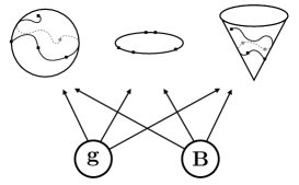
Figure 1: Topologically constrained trajectories driven by a set of common latent forces.

While the extension to geometrically structured, non-Gaussian, trajectories allows for increased modelling capabilities, there is no longer a simple closed form solution for the pathwise trajectories analogous to (2). Indeed, the analogous pathwise solution may be given by the expansion

$$\mathbf{x}(t)=\bigg{(}I +\int_{t_{0}}^{t}\mathbf{A}(\tau)\mathrm{d}\tau$$

$$+\int_{t_{0}}^{t}\mathbf{A}(\tau_{1})\int_{t_{0}}^{\tau_{1}}\mathbf{A}(\tau_{2})\mathrm{d}\tau_{2}\mathrm{d}\tau_{1}+\cdots\bigg{)}\mathbf{x}(t_{0}).$$ (5)

The presence of products of the matrix GP within each of the integrands make it unclear as to how the distribution of the GP terms will propagate to the state space, and unlike the case for (2) it may not be possible to marginalise over these variables. Because we cannot perform this marginalisation step we will, in the remainder of this paper, consider methods for approximating the conditional distributions around a given sample of the latent GPs.

3 ADAPTIVE GRADIENT MATCHING

Bayesian adaptive gradient matching methods were introduced in [Calderhead et al., 2009, Dondelinger et al., 2013] for carrying out approximate inference of the evolution of a $K$-dimensional state variable described by the very general class of, possibly nonlinear, ODEs

$$\frac{\operatorname{d}\mathbf{x}(t)}{\operatorname{d}t}=f(\mathbf{x},\boldsymbol{\theta}),$$ (6)

where the smooth function $f(\cdot;\boldsymbol{\theta})$ is parametrised by some random vector $\boldsymbol{\theta}$. While initially applied to the inference of a finite dimensional parameter vector it is, in principle, straightforward to extend the approach to the infinite dimensional case.

We shall be interested in carrying out posterior inference on the basis of a collection of $\mathbb{R}^{K}$ valued random variables $\mathbf{Y}=\{\mathbf{y}(t_{1}),\ldots,\mathbf{y}(t_{N})\}$ observed at times $t_{1}<\cdots<t_{N}$. Each of these variables is assumed to be an independent noisy observation of the state variable, $\mathbf{x}(t)$, the evolution of which is described by (6). We denote the complete collection of state variables by $\mathbf{X}$, and also consider the vectors formed taking only the $k$th dimensional component at each time point which we denote by $\mathbf{x}_{k}:=(\mathbf{x}_{k}(t_{1}),\ldots,\mathbf{x}_{k}(t_{N}))^{\top}$. If will also be convenient to define the $N$-vector $\mathbf{f}$ with components $(\mathbf{f}_{k})_{i}:=(f(\mathbf{x}(t_{i}),\boldsymbol{\theta}))_{k}$, $i=1,\ldots,N$.

Generally speaking, inference for ODE problems with random parameters, is difficult because the state is only given implicitly as a transformation of the stochastic processes. The problem would be simpler if observations of the gradient process were also available because in that case such a transformation is given explicitly by (6). Adaptive gradient matching treats the gradient as a missing variable, and attempts to introduce an approximation to the complete data likelihood which allows for the gradients to be marginalised out. This is done by initially placing independent on each component of the state variable

$$p_{GP}(\mathbf{x}_{k})=\mathcal{N}(\mathbf{x}_{k}\mid\mathbf{0},\mathbf{C}_{\phi_{k}}),$$ (7)

where $\mathbf{C}_{\phi_{k}}$ is the $N\times N$ covariance matrix obtained by evaluating the kernel function of each latent state interpolating process $k(\cdot,\cdot;\phi_{k})$. Each GP is assumed differentiable allowing the construction of a conditional distribution for the gradients, $\dot{\mathbf{x}}_{k}$, under the prior which we denote by

$$p_{GP}(\dot{\mathbf{x}}_{k}\mid\mathbf{x}_{k}):=\mathcal{N}(\mathbf{m}_{\dot{x}_{k}|x_{k}},\mathbf{C}_{\dot{x}_{k}\mid x_{k}}),$$ (8)

where the conditional mean and conditional covariance matrices are obtained from the joint Gaussian distribution of the state and its gradient [Solak et al., 2003].

The conditional distribution (8) contains no reference to the model (6), and therefore [Calderhead et al., 2009] consider introducing a separate conditional density with the nonlinear regression form

$$p_{reg}(\dot{\mathbf{x}}_{k}\mid\mathbf{X},\boldsymbol{\theta},\gamma_{k})=\mathcal{N}(\mathbf{f}_{k}(\mathbf{X},\boldsymbol{\theta}),\gamma\mathbf{I}_{N}),$$ (9)

where $\gamma_{k}$ represents a temperature parameter controlling the extent to which the conditional distribution is constrained by the functional form of the model.

The two dissonant conditional distributions (8) and (9) are then combined to form a single distribution using a product of experts approximation

$$p(\dot{\mathbf{X}}\mid\mathbf{X},\boldsymbol{\theta}) \propto\prod_{k=1}^{K}p_{GP}(\dot{\mathbf{x}}_{k}\mid\mathbf{x})p_{reg}(\dot{\mathbf{x}}_{k}\mid\mathbf{f}_{k}(\mathbf{X},\boldsymbol{\theta}),\gamma_{k}\mathbf{I}_{N}).$$ (10)

The result is a conditional density which places most of its mass around estimates of the gradient which agree with the parametrised model (6), but also coincide with the gradient of a GP interpolant.

Since this distribution is a product of Gaussians it is possible to marginalise over the gradients, [Dondelinger et al., 2013], leading to

$$p(\mathbf{X}\mid\boldsymbol{\theta}) =\int p(\dot{\mathbf{X}},\mathbf{X}\mid\boldsymbol{\theta})\mathrm{d}\mathbf{X}$$

$$\propto\exp\bigg{\{}-\frac{1}{2}\sum_{k=1}^{K}\boldsymbol{\eta}_{k}^{\top}(\mathbf{C}_{\dot{x}_{k}|x_{k}}+\gamma_{k}I)^{-1}\boldsymbol{\eta}_{k}$$

$$\qquad{}\qquad-\frac{1}{2}\mathbf{x}_{k}^{\top}\mathbf{C}_{\phi_{k}}^{-1}\mathbf{x}\bigg{\}},$$ (11)

where we have defined

$$\boldsymbol{\eta}_{k} =\mathbf{f}_{k}-\mathbf{m}_{\dot{x}_{k}|x_{k}}.$$

It is clear that if the evolution equation is a degree $P$ polynomial in the state then the argument of the exponential in (11) will be a degree $2P$ polynomial. Here we consider the linear case which leads to exponential quadratics, and so tractable Gaussian posterior conditionals.

When the evolution equation (6) is given by the MLFM (3) we identify the arbitrary parameter $\boldsymbol{\theta}$ with the set of latent forces $\mathbf{g}=\{\mathbf{g}_{1},\ldots,\mathbf{g}_{R}\}$ and coefficient matrix $\mathbf{B}$. We may rewrite the variable $\mathbf{f}_{k}$ appearing in (11) using the equivalent linear representations

$$\mathbf{f}_{k}=\sum_{j=1}^{K}\mathbf{u}_{kj}\circ\mathbf{x}_{j}=\sum_{r=0}^{R}\mathbf{v}_{kr}\circ\mathbf{g}_{r}=\sum_{r=0}^{R}\sum_{d=1}^{D}\beta_{rd}\mathbf{w}_{rd},$$ (12)

where $\circ$ denotes the elementwise product of two arrays of conforming shape, and we define the $N$-vectors

$$\mathbf{u}_{kj}=\sum_{r=0}^{R}A_{rkj}\mathbf{g}_{r},\qquad\mathbf{v}_{kr}=\sum_{j=1}^{K}A_{rkj}\mathbf{x}_{j},$$

and

$$\mathbf{w}_{rd}=\mathbf{g}_{r}\circ\sum_{d=1}^{D}\sum_{j=1}^{K}\mathbf{L}_{dkj}\mathbf{x}_{j}.$$

Having defined these variables we can produce a posterior for any choice of of the variables $\mathbf{X},\mathbf{g},\mathbf{B}$ by conditioning on $\mathbf{u}$, $\mathbf{v}$ or $\mathbf{w}$ respectively, and then rearranging the exponential quadratic accordingly. It follows that if we also place a Gaussian prior on the coefficient $\mathbf{B}$, we will have a collection of Gaussian posteriors

$$p(\mathbf{X}\mid\mathbf{B},\mathbf{g}) =\mathcal{N}\left(\mathbf{X}\mid\mathbf{0},\mathbf{S}_{x}(\mathbf{B},\mathbf{g})\right),$$ (13a)

$$p(\mathbf{g}\mid\mathbf{X},\mathbf{B}) =\mathcal{N}\left(\mathbf{g}\mid\mathbf{m}_{g}(\mathbf{X},\mathbf{B}),\mathbf{S}_{g}(\mathbf{B},\mathbf{g})\right),$$ (13b)

$$p(\mathbf{B}\mid\mathbf{X},\mathbf{g}) =\mathcal{N}\left(\mathbf{B}\mid\mathbf{m}_{\beta}(\mathbf{X},\mathbf{g}),S_{\beta}(\mathbf{X},\mathbf{g}\right).$$ (13c)

These closed form solutions are in contrast to the general case in which it is necessary to sample from the density (11) with unknown normalising constant.

As an example $S_{g}(\mathbf{X},\mathbf{B})$ is formed by inverting the $R\times R$ block matrix given by

$$S_{g}(\mathbf{X},\mathbf{B})^{-1}_{rs}=\sum_{k=1}^{K}\mathbf{v}_{kr}\mathbf{v}_{ks}^{\top}\circ\left(\mathbf{C}_{\dot{x}_{k}|\dot{x}}+\gamma_{k}I\right)^{-1}+\delta_{rs}\mathbf{C}_{\psi_{r}}^{-1},$$

for $r,s=1,\ldots,R$, and where $\mathbf{C}_{\psi_{r}}$ is the covariance matrix of the $r$th latent force. Similarly, the mean is given by

$$\mathbf{m}_{g}=\mathbf{S}_{g}(\mathbf{X},\mathbf{B})^{-1}\sum_{k=1}^{K}\mathbf{V}_{k}^{\top}(\mathbf{C}_{\dot{x}_{k}|x_{k}}+\gamma_{k}I)^{-1}(\mathbf{m}_{k}-\mathbf{v}_{k,0}).$$ (14)

The construction of the Gaussian conditionals for $\mathbf{B}$ and $\mathbf{X}$ proceeds in a similar way. The fact that each of the variables of principal interest is conditionally Gaussian allows for straightforward implementation of Gibbs sampling methods, or of mean field variational updates.

4 MIXTURES OF SUCCESSIVE APPROXIMATIONS

The key component of the adaptive gradient matching method described in the previous section is the imposition of an approximate fixed point condition for the linear differential operator

$$\mathcal{D}f(t)\stackrel{{\scriptstyle\Delta}}{{=}}\frac{\mathrm{d}f(t)}{\mathrm{d}t}-\mathbf{A}(t)f(t),$$

for differentiable $\mathbb{R}^{K}$ valued functions $f$. This fixed point condition was encoded into the likelihood function through the gradient expert (10). In this section we consider an alternative approach by first integrating the differential equation, and then considering fixed points of the integral operator

$$\mathcal{L}f(t)\stackrel{{\scriptstyle\Delta}}{{=}}f(t_{0})+\int_{t_{0}}^{t}\mathbf{A}(\tau)f(\tau)\mathrm{d}\tau.$$ (15)

We follow the construction in [Tait and Worton, 2018] by considering an approximation to the distribution of the state variable $\mathbf{x}(t)$ conditional on dense sample paths of the coefficient matrix $\mathbf{A}(t)$. The solution will be constructed from a given initial approximation $\mathbf{x}^{(0)}$ by means of the Picard iteration

$$\mathbf{x}^{(n+1)}(t)=\mathbf{x}^{(n)}(t_{0})+\mathcal{K}[\mathbf{x}^{(n)}](t),$$ (16)

where the integral operator is defined by

$$\mathcal{K}[f](t)\stackrel{{\scriptstyle\Delta}}{{=}}\int_{t_{0}}^{t}\mathbf{A}(\tau)f(\tau)\mathrm{d}\tau.$$ (17)

Repeatedly iterating the map (16) from a constant initial approximation, and then collecting terms leads to the expansion (5). This approach is referred to as the method of successive approximations, and is an important construction in the classical existence and uniqueness theorems for ODEs.

In practice we have access to only a finite realisation of the sample path of the coefficient matrix, although we may make this path arbitrarily fine at a corresponding increase in computational complexity. Therefore assuming a suitably fine approximation we may replace the integral (17) with a numerical quadrature

$$\mathcal{K}[\mathbf{x}](t_{n})\approx\sum_{i=1}^{N}w_{ni}\mathbf{A}(t_{i})\mathbf{x}_{i},$$ (18)

for appropriate choice of quadrature weights $w_{ni}$. Then a discretisation of the operator $\mathcal{K}$ is given by

$$\mathbf{K}[\mathbf{g},\mathbf{B}] =\sum_{n=0}^{N}\mathbf{w}_{n}\mathbf{e}_{n}^{T}\otimes\mathbf{A}(t_{n})$$

$$=\sum_{n=0}^{N}\left[\sum_{d=1}^{D}(\beta_{0d}+\sum_{r=1}^{R}g_{rn}\beta_{rd})\cdot\mathbf{w}_{n}\mathbf{e}_{n}^{\top}\otimes\mathbf{L}_{d}\right].$$ (19)

The corresponding discretisation of the transformation (16), which we shall denote by $\mathbf{P}_{\nu}=\mathbf{P}_{\nu}[\mathbf{g},\mathbf{B}]$, may be formed by choosing an index $\nu\in\{1,\ldots,N\}$ which will correspond to the initial time. The $K$-vector $\mathbf{x}(\tau_{\nu})$ is invariant under (16) and so we may consider the discrete approximation to this transformation which will act on block vectors of the form $\mathbf{v}=(\mathbf{v}_{1},\ldots,\mathbf{v}_{N})^{\top}$ with $\mathbf{v}_{i}\in\mathbb{R}^{K}$ for $i=1,\ldots,N$, by the matrix/vector operation

$$\mathbf{P}\mathbf{v}=\mathbf{v}_{\nu}\otimes\mathbf{1}_{N}+\mathbf{K}[\mathbf{g},\boldsymbol{\beta}]\mathbf{v}.$$ (20)

As a single iteration of the map (16) only produces a first order approximation to the solution around $\tau_{\nu}$ it is necessary to consider higher order approximations by taking $M$ iterates of this map, $M\geq 1$. The result is a discrete approximation to an $M$th order truncation of the Neumann series expansion given by (5). This construction allows us to construct approximations to the pathwise solution of the state variable for given latent parameters which will locally solve the IVP around $\tau_{\nu}$. Our approach is to use this local approximation to motivate a regression model for the conditional density of the state variables which takes the form

$$p_{\nu}(\mathbf{X}\mid\mathbf{g},\mathbf{B},\alpha,M)=\prod_{n=1}^{N}\mathcal{N}(\mathbf{x}(t_{n})\mid\mathbf{m}_{\nu,n},\alpha^{-1}\mathbf{I}_{K}),$$ (21)

where $\mathbf{m}_{\nu,n}$ is the $nth$ subvector of the expression

$$\mathbf{m}_{\nu}=\mathbf{P}_{\nu}^{M}(\boldsymbol{\mu}_{\nu}\otimes\mathbf{1}_{N}).$$

Conditional on $\mathbf{g}$ and $\mathbf{B}$, the density function (21) may be viewed as an $M$th order approximation to the IVP (3) with initial condition $\boldsymbol{\mu}_{\nu}$ and precision $\alpha$. The mean function $\mathbf{m}_{\nu}$ will be a degree $M$ polynomial in the values of the latent forces and connection coefficients. The parameters $\boldsymbol{\mu}_{\nu}$ are to be interpreted as initial conditions of a local version of the IVP (3), and for high precision $\alpha$ are well informed by the data.

As the construction is local in character, larger time intervals will necessarily require higher orders of approximation, and therefore an increasing computational burden. In order to alleviate this complexity rather than model the whole interval with one conditional density, our approach is to pick a set of initial times $\tau_{\nu},\nu=1,\ldots,D$, and consider the mixture of local regression models

$$p(\mathbf{X}\mid\mathbf{g},\boldsymbol{\beta},\alpha)=\sum_{\nu=1}^{D}\pi_{\nu}p_{\nu}(\mathbf{X}\mid\mathbf{g},\boldsymbol{\beta},\alpha).$$ (22)

Each mixture component represents a local approximation to the solution of the MLFM around $\tau_{\nu}$. We refer to approaches using the likelihood term (22) as MLFM by mixtures of successive approximations (MLFM-MixSA) methods. After introducing priors for the latent variables it is straightforward to construct maximum a posteriori (MAP) estimates using the standard Expectation-Maximisation (EM) approach for Gaussian mixture models. The classical EM approach to fitting mixtures of Gaussians introduces the responsibility variables and in this instance will act to discover regions over which an $M$th order truncation of the expansion (5) gives a good approximation to the solution.

5 SIMULATION STUDY

The construction of the MLFM-AG using interpolation of the state variables, and the construction of the MLFM-MixSA using local approximations suggests the need to investigate these methods under two regimes; the first is the effect of the spacing $\Delta t$ between observations, and the second the impact of the interval length each mixture component is accounting for. For the studies in this section we investigate both of these regimes while holding the total sample size constant, for each experimental setting we simulate a total of $100$ experiments and report the average error.

5.1 Kubo oscillator

For models in which the Lie algebra is trivial it is possible to motivate a MAP estimate of the LF under an approximation to the true posterior. One such case is the random harmonic oscillator, [van Kampen, 2007] defined as the complex-valued ODE

$$\dot{z}(t)=-ig(t)z(t),\qquad z(t_{0})\in S^{1}\subset\mathbb{C}.$$ (23)

We use the methods introduced in this paper to construct MAP estimates of the latent forces which we compare with the estimates obtained using an approximation to the true conditional density considered in [Tait and Worton, 2018]. For the MLFM-MixSA we fix the approximation order at $M=5$ and consider the effiect of varying the number of mixtures with equally spaced initial times $\tau_{\nu},$ $\nu=1,\ldots D$ with $D\in\{1,2,3\}$.

The results are displayed in Table 1 and show that the adaptive gradient matching methods perform very well when the sampling frequency is high, but the performance deteriorates as $\Delta t$ decreases. The ability to increase the number of mixture centers in the MLFM-MixSA model allows this method to better deal with the case when the data is sparse relative to the system complexity.

Because the MLFM-AG method is constructed around interpolating functions it is not the frequency itself that leads to the decrease in performance, but the likely increase in distance between points as the time between them increases and a corresponding information loss in the interpolating functions. The loss of structural information for GP interpolants on manifolds is displayed in Figure 2(a). In Figure 2(b) we see that as the average arc length between data points increases the performance of the MLFM-AG methods deteriorate.

Table 1: $\|\cdot\|_{2}$ distance of the latent force MAP estimates from the ground truth value on the interval $[0,6]$. Reported are the results using the MLFM-AG and order $M=5$ MLFM-MixSA approximation.

$\Delta t$	MLFM-AG	MLFM-MixSA
		$D=1$	$D=2$	$D=3$
$0.50$	0.237	2.128	0.449	0.319
$0.75$	0.402	2.006	0.489	0.410
$1.00$	0.640	1.816	0.575	0.528

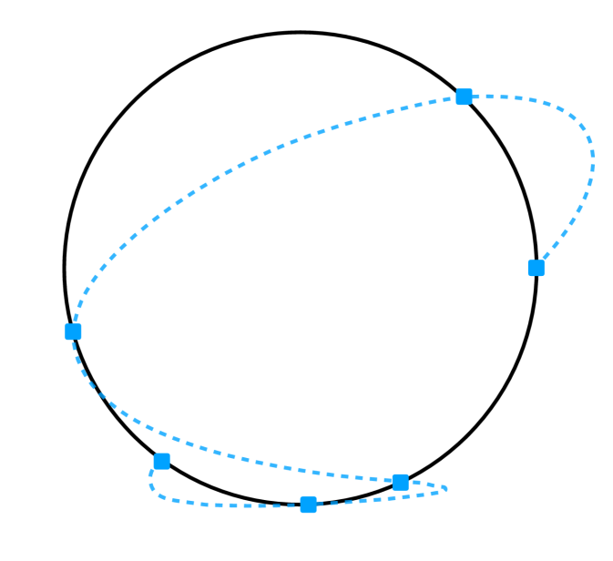
(a) GP interpolant

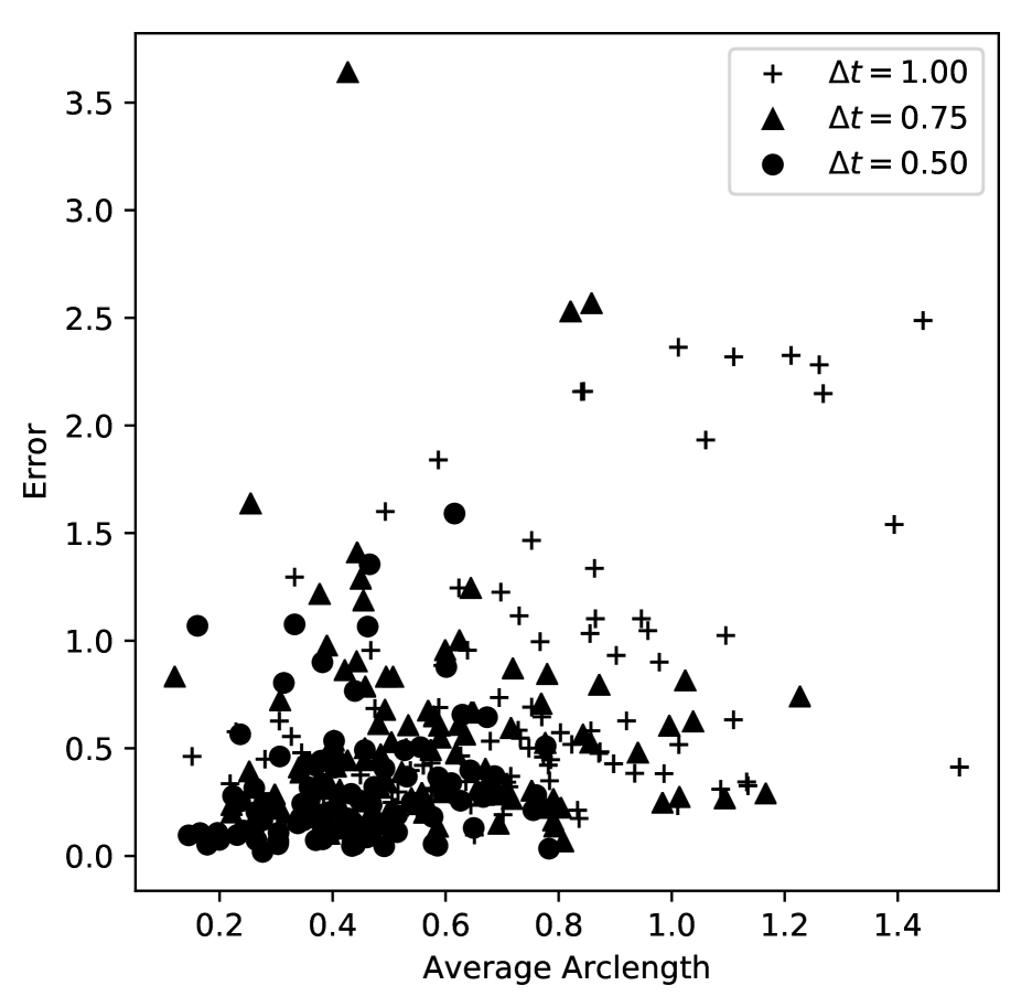
(b) Error vs. arc length

Figure 2: (a) GP functions on $S^{1}$ perform poorly as distance between points increases. (b) The accuracy of the MLFM-AG approaches depends on the interpolating process, and so diminishes with the average arc length between points.

5.2 Dynamic systems on SO(3)

The MLFM framework enables the modelling of the action of a group on a vector space, important to this process will be the ability to learn the coefficient matrix of the IVP corresponding to the fundamental solution

$$\frac{\mathrm{d}\mathbf{x}(t)}{\mathrm{d}t}=\mathbf{A}(t)\mathbf{x}(t),\qquad\mathbf{x}(t_{0})=\mathbf{I}_{K}.$$ (24)

For this example we consider the case $\mathbf{A}(t)\in\mathfrak{so}(3)$, the Lie algebra of infinitesimal rotations of $\mathbb{R}^{3}$.

The skew-symmetry conditions of the matrix $\mathbf{A}(t)$ imply there are only three independent components $\{a_{12}(t),a_{13}(t),a_{2,3}(t)\}$, the remaining being fixed by the skew-symmetry condition. Therefore we allow $\mathbf{B}$ and $\mathbf{g}$ to vary freely and compare both methods introduced in this paper to estimating these functions. We simulate each system using one latent force and each $\boldsymbol{\beta}_{r},r=0,1$ distributed uniformly on the sphere $S^{2}$. Because it is no longer possible to derive the ground truth MAP estimates we shall instead consider the ‘reconstruction error’ for the IVP at the MAP estimates which we define to be the $\|\cdot\|_{2}$ between the true samples and the result from solving the ODE with the MAP estimates.

The results are displayed in Table 2 and for the MLFM-AG model the same general conclusions hold; the method performs very well with $\Delta t$ small, and diminishes in performance as this increases. For the MLFM-MixSA model we again observe that when data is sparse relative to the model structure the greater adaptive potential of this method allows for more accurate results, we also observe a diminishing benefit to increasing the approximation order.

Table 2: Reconstruction error solving the ODE (24) on the interval $[0,6]$ using the MAP estimates obtained via the MLFM-AG and the MLFM-MixSA methods, with two mixture components

$\Delta t$	MLFM-AG	MLFM-MixSA
		$M=3$	$M=5$	$M=7$
0.50	0.110	0.487	0.212	0.167
0.75	0.252	0.611	0.276	0.233
1.00	0.419	0.570	0.410	0.355

6 APPLICATION: MOCAP DATASET

Motion capture data for human poses typically consists of a representative ‘skeleton’, the bone segments of which are given by an orientation vector in a local reference frame. The motion series is then given by rotations of these initial configurations, typically recorded as Euler angles. These angles may be represented by an equivalent unit quaternion [Whittaker and McCrae, 1988] and so, up to an antipodal equivalence, identified with the sphere $S^{3}\subset\mathbb{R}^{4}$.

For this experiment we first train the MLFM for the marginal time series of each joint segment with joint specific latent variables. We use the data from motions 1–5 of subject $64$ from the Carnegie Mellon mocap dataset. We estimate the prediction error using leave-one-out cross validation, the results of four joints are displayed in Figure 3 which show that typically at two latent forces are sufficient.

For the quaternion valued time series of each joint we have dimension $K=4$, and accurate reconstructions requires $R\geq 2$, as a latent variable model this is a very modest dimension reduction. To realise the full benefit of the latent variable modelling approach we now consider using the product topology structure of the MLFM as described in Section 2 by allowing each of the joints to share information through the common GPs. The results of fitting the product MLFM with $R\in\{3,4\}$ forces are also displayed in Figure 3. The prediction error for the multiple joint MLFM is given by the horizontal lines, and by sharing information between the set of common forces we observe that the point estimates of the model with $4$ latent forces outperforms the marginal joint prediction errors. The product MLFM structure therefore allows not only for a latent variable dimensionality reduction, but also the sharing of information between the joints leads to improved generalisation and a better predictive performance.

(a) Left humerus

(b) Right humerus

(c) Left femur

(d) Right femur

Figure 3: Cross validation estimates of the prediction error. The error bars give the $\pm$ one standard deviation of the prediction error for each joint with $R$ latent forces fitting the MLFM with only data for that joint. The horizontal ‘ ’ line gives the prediction error using the combined model with $3$ forces and ‘ ’ gives the result using $4$ forces.

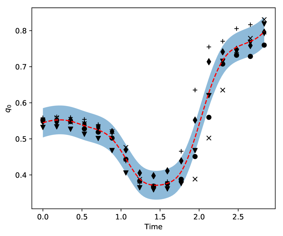
(a) Left humerus, $q_{0}$

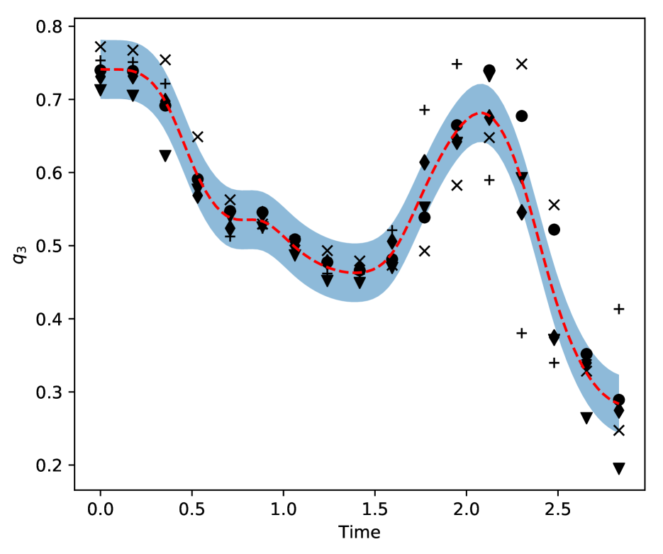
(b) Left humerus, $q_{3}$

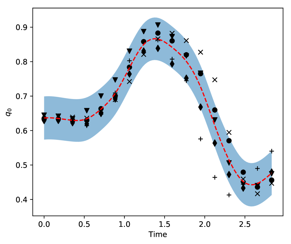
(c) Right humerus, $q_{0}$

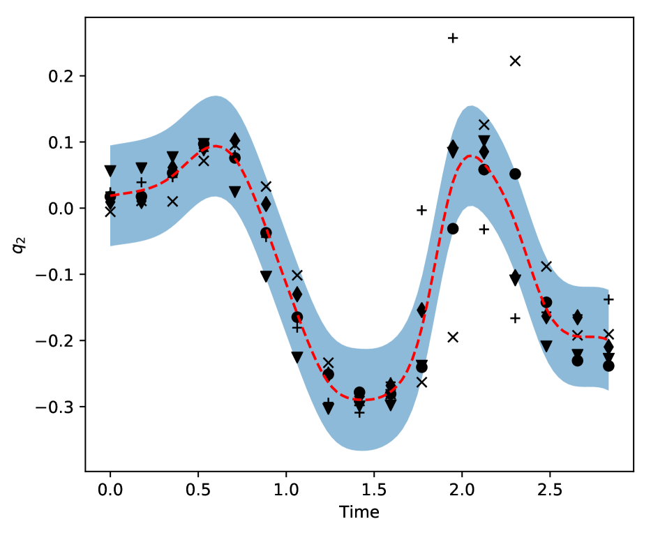
(d) Right humerus, $q_{2}$

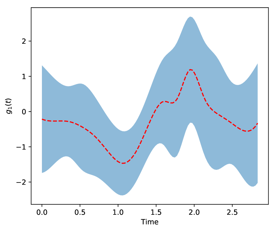
(e) Right humerus, latent force 1

(f) Multiple joint, latent force 2

Figure 4: Inferred motions and latent forces for subject 64 from motions 1–5.

7 DISCUSSION

We have described the MLFM, a semi-parameteric modelling approach for dynamic systems allowing for strong geometric constraints to be combined with flexible GP terms. The models provides a useful framework for modeling trajectories on distinct manifolds sharing information through a common set of latent GPs, and our application to motion capture data in Section 6 indcates that this process of information sharing leads to better predictive performance than the marginal models. To conduct inference in this class of models we have introduced two methods of constructing approximate conditional distributions. The first approximation was based on the use of adaptive gradient matching methods, and the second motivated by the method of successive approximations.

The MLFM-AG method is to be preferred in terms of computational efficiency, however while our simulation studies presented in Section 5 suggest this method performs very well on densely sampled data, this performance deteriorates when the data is sparse relative to the model complexity. In particular the GP interpolants on which the model are constructred are unable to capture the proper manifold structure over longer distances in the data space, Figure 2(a). In connection with this it should be emphasised that any concerns of this type in the linear setting will also manifest in the more general nonlinear setting, and therefore embedding known structure and preserved quantities into gradient matching methods seems an important area of future research.

The construction of the MLFM-MixSA involved discrete tuning parameters in the truncation order, $M$, and the number of mixture components. The method is computationally more burdensome, but the simulation studies suggest this cost may be necessary to achieve accurate inference. It is possible to intepret the Picard iterations (16) as a linear dynamic system, with the approximation order as the temporal variable. Future research may demonstrate that this may be used to motivate an efficient approximation to the density (21), also allowing for variational approaches.

One of the attractive features of the MLFM is that nonlinear changes in the model geometry become dimensionality changes in an associated vector space. This suggests a framework for carrying out the process of latent manifold discovery by transforming the original problem to one in a vector space setting. In future work we aim to apply this method to learn topologically constrained latent variable models, [Urtasun et al., 2008], in constrast to the a priori assumption of a known geometry in this work.

Acknowledgements

Daniel J. Tait is supported by an EPSRC studentship.

References

- [Alvarez et al., 2009] Alvarez, M., Luengo, D., and Lawrence, N. (2009). Latent force models. In van Dyk, D. and Welling, M., editors, Proceedings of the Twelth International Conference on Artificial Intelligence and Statistics, volume 5 of Proceedings of Machine Learning Research, pages 9–16, Hilton Clearwater Beach Resort, Clearwater Beach, Florida USA. PMLR.
- [Calderhead et al., 2009] Calderhead, B., Girolami, M., and Lawrence, N. D. (2009). Accelerating bayesian inference over nonlinear differential equations with Gaussian processes. In Koller, D., Schuurmans, D., Bengio, Y., and Bottou, L., editors, Advances in Neural Information Processing Systems 21, pages 217–224. Curran Associates, Inc.
- [Dondelinger et al., 2013] Dondelinger, F., Husmeier, D., Rogers, S., and Filippone, M. (2013). Ode parameter inference using adaptive gradient matching with Gaussian processes. In Carvalho, C. M. and Ravikumar, P., editors, Proceedings of the Sixteenth International Conference on Artificial Intelligence and Statistics, volume 31 of Proceedings of Machine Learning Research, pages 216–228, Scottsdale, Arizona, USA. PMLR.
- [Hall, 2015] Hall, B. C. (2015). Lie Groups, Lie Algebras and Representations. Graduate Texts in Mathematics. Springer.
- [Iserles and Nørsett, 1999] Iserles, A. and Nørsett, S. P. (1999). On the solution of linear differential equations in Lie groups. Philosophical Transactions: Mathematical, Physical and Engineering Sciences, 357(1754):983–1019.
- [Solak et al., 2003] Solak, E., Murray-smith, R., Leithead, W. E., Leith, D. J., and Rasmussen, C. E. (2003). Derivative observations in Gaussian process models of dynamic systems. In Becker, S., Thrun, S., and Obermayer, K., editors, Advances in Neural Information Processing Systems 15, pages 1057–1064. MIT Press.
- [Tait and Worton, 2018] Tait, D. J. and Worton, B. J. (2018). Multiplicative latent force models. ArXiv e-prints, page arXiv:1811.00423.
- [Urtasun et al., 2008] Urtasun, R., Fleet, D. J., Geiger, A., Popović, J., Darrell, T. J., and Lawrence, N. D. (2008). Topologically-constrained latent variable models. In Proceedings of the 25th International Conference on Machine Learning, ICML ’08, pages 1080–1087, New York, NY, USA. ACM.
- [van Kampen, 2007] van Kampen, N. G. (2007). Stochastic Processes in Physics and Chemistry. Elsevier, 3 edition.
- [Whittaker and McCrae, 1988] Whittaker, E. T. and McCrae, S. W. (1988). A Treatise on the Analytical Dynamics of Particles and Rigid Bodies. Cambridge Mathematical Library. Cambridge University Press.