Detection of Circumstellar Helium in Type Iax Progenitor Systems

Abstract

We present direct spectroscopic modeling of 44 Type Iax supernovae (SNe Iax) using spectral synthesis code SYNAPPS. We confirm detections of helium emission in the early-time spectra of two SNe Iax: SNe 2004cs and 2007J. These He i features are better fit by a pure-emission Gaussian than by a P-Cygni profile, indicating that the helium emission originates from the circumstellar environment rather than the SN ejecta. Based on the modeling of the remaining 42 SNe Iax, we find no obvious helium features in other SN Iax spectra. However, $\approx 76\%$ of our sample lack sufficiently deep luminosity limits to detect helium emission with a luminosity of that seen in SNe 2004cs and 2007J. Using the objects with constraining luminosity limits, we calculate that 33% of SNe Iax have detectable helium in their spectra. We examine 11 SNe Iax with late-time spectra and find no hydrogen or helium emission from swept up material. For late-time spectra, we calculate typical upper limits of stripped hydrogen and helium to be $2\times 10^{-3}\ {\rm M}_{\odot}$ and $10^{-2}\ {\rm M}_{\odot}$, respectively. While detections of helium in SNe Iax support a white dwarf-He star binary progenitor system (i.e., a single-degenerate [SD] channel), non-detections may be explained by variations in the explosion and ejecta material. The lack of helium in the majority of our sample demonstrates the complexity of SN Iax progenitor systems and the need for further modeling. With strong independent evidence indicating that SNe Iax arise from a SD channel, we caution the common interpretation that the lack of helium or hydrogen emission at late-time in SN Ia spectra rules out SD progenitor scenarios for this class.

1 Introduction

Type Iax supernovae (SNe Iax) are a recently defined class of stellar explosion (Foley et al., 2013) that share similar characteristics to their common cousins, SNe Ia. However, SNe Iax exhibit lower peak luminosities and ejecta velocities than SNe Ia. There exist ${\sim}50$ confirmed SNe Iax to date (Jha, 2017), all spectroscopically similar to the prototypical SN Iax, SN 2002cx (Li et al., 2003). As is the case for SNe Ia, the progenitor system and explosion mechanisms of SNe Iax are still unclear.

Due to their spectroscopic agreement with SNe Ia near maximum light, SNe Iax are generally considered to be thermonuclear explosions that result from a white dwarf (WD) in a binary system. Based on stellar population estimates (Foley et al., 2009; McCully et al., 2014), SNe Iax are found in younger stellar populations with ages ${\leq}100$ Myr (Lyman et al. 2013; Lyman et al. 2018; Takaro et al. 2019). In terms of a progenitor channel, these short evolutionary timescales indicate that SNe Iax may be the result of more massive WDs in a binary system with a non-degenerate companion such as a He star (Iben & Tutukov, 1994; Hachisu et al., 1999; Postnov & Yungelson, 2014; Jha, 2017). This type of system has been modeled by Liu et al. (2010) where the final binary stage consists of a $1\ {\rm M}_{\odot}$ C/O WD and a $2\ {\rm M}_{\odot}$ He star (see also Yoon & Langer, 2003; Wang et al., 2015; Brooks et al., 2016). The WD then accretes helium from its binary companion and explodes as it approaches the Chandrasekhar mass (Jha, 2017). From model predictions, SN Iax explosions most resemble pure deflagrations in which the explosion energy is not enough to completely unbind the star (Jordan et al., 2012; Kromer et al., 2013; Fink et al., 2014).

The recent pre-explosion detection of a blue point source coincident with SN 2012Z provides strong support for the C/O WD + He star progenitor scenario for SNe Iax (McCully et al., 2014). Such a system would have a significant amount of He on the WD surface, in the outer layers of the donor, and possibly in the circumstellar environment. Therefore under certain conditions, one might detect He features in a SN Iax spectrum. In fact, He lines have been detected in the spectra of two SNe Iax: SN 2004cs and SN 2007J (Filippenko et al., 2007; Foley et al., 2009, 2013; Foley et al., 2016). Both objects being spectroscopically SNe Iax, their spectra display prominent He i $\lambda\lambda$ 5875, 6678, 7065, and 7281 emission lines and minor He i features at bluer wavelengths.

Since the classification of SNe 2004cs and 2007J as SNe Iax, there have been arguments put forward that these objects should be classified as SNe IIb (White et al., 2015). However, this claim is addressed in detail by Foley et al. (2016), who compare the spectral epochs of SNe 2007J and 2002cx to that of SNe IIb, including SN 1999cb, which had an extremely weak H-$\alpha$ emission at late times. Foley et al. (2016) showed noticeable differences between SN 2007J and SNe IIb and detect no hydrogen lines in any SN 2007J spectra. Additionally, Foley et al. (2016) show that the light curve of SN 2004cs does not match that of any SN IIb template, further differentiating SNe Iax with helium lines and SNe IIb.

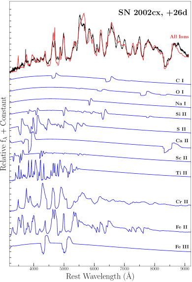
Figure 1: Decomposition of all active ions in a SYNAPPS fit shown in blue. In black, spectral data SN 2002cx at +26d after maximum light. SYNAPPS fit to data shown in red.

The detection of He emission in two SNe that, other than their He emission, are spectroscopically and photometrically similar to other SNe Iax suggest that faint, thus-far undetected He features may be present in spectra of other SNe Iax. One method for detecting helium in SNe Iax is through spectral fitting by radiative transfer simulations such as SYNOW (Parrent, 2014), SYN++/SYNAPPS (Thomas et al., 2011) and TARDIS (Kerzendorf & Sim, 2014). Such an analysis has proven effective in modeling SN Iax spectra and is a viable option in determining the relative strengths of ions in these systems (Branch et al., 2004; Jha et al., 2006; Stritzinger et al., 2014; Szalai et al., 2015; Barna et al., 2018). Furthermore, Magee et al. (2019) used TARDIS to model the spectra of six SNe Iax, including one spectrum of SN 2007J, to search for signatures of photospheric helium in these objects. Magee et al. (2019) was able to reproduce the basic He i features in the first spectral observation of SN 2007J by including significant amounts of helium in the photosphere. We discuss the relevance and implications of these models in Section 5.3. By applying a similar analysis (i.e., parameterized spectral synthesis codes) here, we can comprehensively search for helium emission for most of the SN Iax sample.

In Section 2, we introduce our early- and late-time sample of SNe Iax. In Section 3, we outline our method for searching for He i emission in SNe Iax at early-times. In Section 4, we examine the late-time spectra for hydrogen and helium emission as it relates to the SN Iax progenitor system. We discuss our results in Section 5 and conclude in Section 6.

2 SNe Iax Sample

Through Jha (2017) and the Open Supernova Catalog (Guillochon et al., 2017), we identified 54 spectroscopically confirmed SNe Iax, and we use this list to build our sample. We were able to obtain 110 spectra of 44 SNe Iax. We performed SYNAPPS fitting for all spectra with a phase of $\lesssim$78 days relative to peak brightness. We present all spectra with phases and references in Tables 2 & 3. The majority of spectral phases shown are relative to B band maximum. If B band photometry is unavailable for a given object, we use the relations presented in Table 6 of Foley et al. (2013) to convert all spectral phases to be relative to maximum light in B band. For objects without adequate photometry, we perform a spectral comparison to other SNe Iax using the Supernova Identification package (SNID; Blondin & Tonry 2007) to estimate each spectral phase. We caution the direct use of spectral phases calculated using SNID due to the small sample size of SNe Iax able to be used in determining these phase range estimates in addition to the overall uncertainty associated with the identification package.

SN 2007J is one such object that does not have as constraining of a light curve as its spectral epochs. For this object, we attempt to match its clear band photometry to the light curve of SN 2004cs in order to calculate a range of possible dates for maximum light. We then use SNID to further constrain the time of maximum when estimating the phases of each spectrum presented.

From this subsample, there are 25 SNe Iax (and 69 spectra) with sufficient photometric data to properly flux calibrate the spectra. We also examined 24 late-time spectra of 11 SNe Iax with sufficient photometry to flux calibrate the spectra. The late-time spectra range in phase from 103 to 461 days after peak brightness.

3 Early-time Helium Emission

3.1 Spectroscopic Analysis

To model the spectral features in early-time, “photospheric” SN Iax spectra, we apply radiative transfer codes SYNAPPS and SYN++ (Thomas et al., 2011). Both being parameterized spectral synthesis codes, SYNAPPS performs an automated, $\chi^{2}$ minimization fit to the data while SYN++ requires manual adjustment of available parameters. For each active ion in a given fit, the parameters used include: optical depth ($\tau$), specific line velocity limits ($v_{\textrm{min}}/v_{\textrm{max}}$), e-folding length for the opacity profile, and Boltzmann excitation temperature ($T_{\textrm{exc}}$). General input parameters for SYN++/SYNAPPS are photospheric velocity ($v_{\textrm{phot}}$), outermost velocity of the line forming region ($v_{\textrm{outer}}$) and blackbody temperature of the photosphere ($T_{\textrm{BB}}$). While SYN++/SYNAPPS are built on multiple assumptions about the SN explosion such as spherical symmetry, local thermal equilibrium, and homologous expansion of ejecta (Thomas et al., 2011; Parrent, 2014), they are both excellent tools for accurate line identification.

SYNAPPS models photospheric species in LTE and because of its assumption that the lines are formed above an expanding photosphere, the code produces P-Cygni profiles. Because of its general assumptions about the modeled explosion, SYNAPPS may at times be unable to reproduce the line strengths of ions within the photosphere. However, as discussed above, its accuracy in modeling specific P-Cygni line profiles allows for direct identification of all photospheric species present within a given SN. Furthermore, because of its LTE condition, SYNAPPS cannot accurately reproduce the relative fluxes in NLTE species such as He i, but should be able to reproduce the profile shape. A complete treatment of the NLTE He i species requires specific ionization conditions in order for accurate line strength reproduction through radiative transfer (Hachinger et al., 2012; Dessart & Hillier, 2015; Boyle et al., 2017).

For our spectral modeling, we primarily use SYNAPPS in order to find the best, unbiased fit to the data. Each free parameter discussed above has a range of values that SYNAPPS fits freely without prior constraint. The ranges for each parameter are as follows: $v_{\textrm{min}}=0.20-5\times 10^{3}\ \textrm{km}\,\textrm{s}^{-1}$, $v_{\textrm{max}}=5-15\times 10^{3}\ \textrm{km}\,\textrm{s}^{-1}$, $v_{\textrm{phot}}=1-15\times 10^{3}\ \textrm{km}\,\textrm{s}^{-1}$, $v_{\textrm{outer}}=1-20\times 10^{3}\ \textrm{km}\,\textrm{s}^{-1}$, $T_{\textrm{BB}}=1-15\times 10^{3}$ K,  $\tau=10^{-3}-10^{5}$,  aux $=0.10-15$, and $T_{\textrm{exc}}=1-25\times 10^{3}$ K. Multiple iterations are performed for a given spectrum if a local minimum appears to be reached rather than a global minimum. In this case, we test a range of starting values for each parameter to confirm that their convergence to a given value is authentic. In each fit, we include the following ions: C ii, O i, Na i, Si ii, S ii, Ca ii, Sc ii, Ti ii, Cr ii, Fe ii and Fe iii. All ions are weighted equally and are given identical upper and lower boundaries for each free parameter when fitting. An example of spectral decomposition of fitted ions is shown in Figure 1.

3.2 Helium Line Profile Shape

We first examine the He i features in the spectra of SNe 2004cs and 2007J to further understand what might be present in other spectra. When fitting these spectra with SYNAPPS, we noticed that the He i features were poorly fit. In particular, the P-Cygni absorption should be much stronger (or the emission should be much weaker) than observed. Furthermore, the He i features are more symmetric, relative to zero velocity, than other features in the spectrum. While the synthetic SYNAPPS spectra (blue line in Figure 2) are generally reasonable matches to the data, the helium P-Cygni profiles cannot reproduce the large emission features for He i $\lambda\lambda$7065,7281 — these helium lines are best fit with Gaussian emission features. Other species (e.g., O i; see Figure 3) are, however, well matched to a P-Cygni profile.

For reference, we plot the velocities of O i $\lambda$7774 and He i $\lambda$7065 in Figure 3(a). We show that the absorption profile of oxygen is best represented by a P-Cygni profile while He i is best described by a Gaussian for the $+33-46$-day spectrum of SN 2007J and the +45-day spectrum of SN 2004cs. We also note that for SN 2007J at a later phase of $+65-78$ days, both O i and He i $\lambda$7065 are best defined as Gaussian profiles as the SN ejecta becomes more optically thin.

Because a standard SYNAPPS fit cannot reproduce the helium emission observed, we can fit the spectra with certain regions masked, where SYNAPPS will predict the spectrum in the masked regions. This process allows for a way to examine the complicated continuum at the position of helium features without being influenced by any possible helium emission or absorption. This is applied as we fit the SNe 2004cs and 2007J spectra with SYNAPPS, masking the He i features, and then including additional Gaussian line profiles for each He i feature. The result is presented as the red line in Figure 2. The resulting profile parameters are presented in Table 1.

As an example, we plot the velocities of the 7065Å He i line for both objects at multiple epochs in Figure 3(b). Gaussian emission and P-Cygni profiles are over-plotted in red and blue, respectively. We see that the Gaussian profiles are a better description for all He i lines in both objects. In some cases, the P-Cygni profiles are also too narrow to fit the He i emission.

Furthermore, the peaks of the He i lines in SNe 2004cs and 2007J are both redshifted and blueshifted about rest velocity. This indicates that the helium emitting region may be kinematically decoupled from the SN ejecta and that the system’s helium is not constrained to the photosphere as is needed for a P-Cygni profile. This then strengthens the case for pure He i emission manifesting as a Gaussian line profile in both SNe Iax. All helium line widths and shifts are presented in Table 1.

Table 1: Helium Line Luminosities and Velocities for SNe 2007J and 2004cs

Object	Phase	$\lambda 5876$ Lum.	$\lambda 6678$ Lum.	$\lambda 7065$ Lum.	$\lambda 7065$ Lum.	FWHM $\lambda 5876$	FWHM $\lambda 6678$
	(days)	($10^{38}\rm{ergs\ s}^{-1}$)	($10^{38}\rm{ergs\ s}^{-1}$)	($10^{38}\rm{ergs\ s}^{-1}$)	($10^{38}\rm{ergs\ s}^{-1}$)	($\textrm{km}\,\textrm{s}^{-1}$)	($\textrm{km}\,\textrm{s}^{-1}$)
SN 2007J	5-18	1.027	3.364	7.893	N/A	458.8	887.6
SN 2007J	9-22	15.50	10.16	16.97	2.214	8367	4402
SN 2007J	33-46	12.37	8.453	19.25	9.979	6918	4673
SN 2007J	65-78	2.319	1.532	7.135	4.389	4558	3879
SN 2004cs	45	4.389	4.066	10.21	5.523	3465	2933
Object	Phase	Shift $\lambda 5876$	Shift $\lambda 6678$	Shift $\lambda 7065$	Shift $\lambda 7281$	FWHM $\lambda 7065$	FWHM $\lambda 7281$
	(days)	($\textrm{km}\,\textrm{s}^{-1}$)	($\textrm{km}\,\textrm{s}^{-1}$)	($\textrm{km}\,\textrm{s}^{-1}$)	($\textrm{km}\,\textrm{s}^{-1}$)	($\textrm{km}\,\textrm{s}^{-1}$)	($\textrm{km}\,\textrm{s}^{-1}$)
SN 2007J	5-18	27.48	-204.1	-270.8	N/A	1407	N/A
SN 2007J	9-22	2986	1337	397.4	1305	4193	3735
SN 2007J	33-46	2385	691.2	744.6	1121	4352	3596
SN 2007J	65-78	1708	839.9	588.9	1201	4725	4379
SN 2004cs	45	938.6	-294.4	-449.8	-72.11	3878	4446

To test the White et al. (2015) suggestion that SNe 2004cs and 2007J are SNe IIb, we perform SYNAPPS fits with prominent Balmer lines masked out. We fit the $+9-22$, $+33-46$, and $+65-78$-day spectra for SN 2007J and the +45-day spectrum of SN 2004cs. These fits include all ions listed in Section 3.1 as well as He i. From Figure 4, we see no hydrogen feature in any spectrum (excluding contaminating galactic H-$\alpha$ emission feature for SN 2004cs).

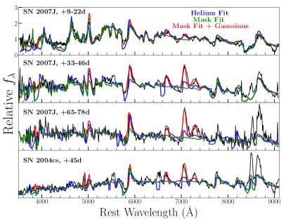
Figure 2: In blue, SYNAPPS fit with active He i ion. In red, SYNAPPS fit with masked out He i regions plus Gaussian emission profiles.

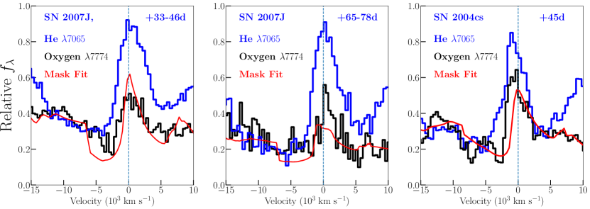
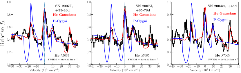
Figure 3: (a) Histogram velocity plot of He $\lambda 7065$ and O $\lambda 7774$ spectral lines for comparison of absorption profiles. Red line is SYNAPPS mask fit plus helium Gaussians, centered on the O $\lambda 7774$ line. (b) $\lambda 7065$ helium line velocity for SN 2007J and SN 2004cs. Red line shows SYNAPPS mask fit with all active ions plus Gaussian profiles at prominent He i lines. Blue line is manually generated SYN++ fit to the He $\lambda 7065$ line with no other active ions present. Refer to the blue line in Figure 2 for the SYNAPPS fit with all active ions and helium.

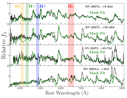
Figure 4: In green, SYNAPPS fits to all epochs of SN 2004cs and SN 2007J with prominent Balmer lines masked out. Region about H $\alpha$ shown in red, H $\beta$ in blue, H $\gamma$ in green, and H $\delta$ in orange.

3.3 Fitting Early-time Spectra

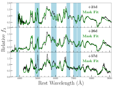
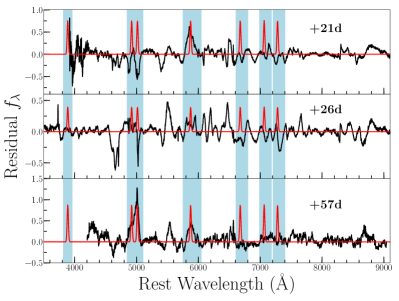
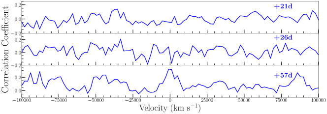
Figure 17: SN 2002cx. Phase relative to B band maximum.

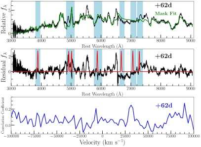
Figure 18: SN 2003gq. Phase relative to B band maximum.

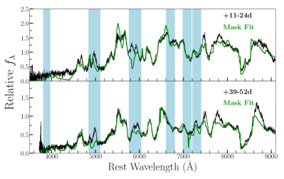
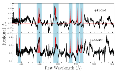
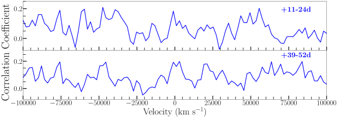
Figure 19: SN 2004gw. Phase relative to B band maximum and calculated using SNID.

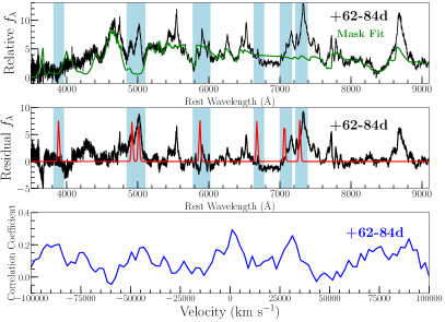
Figure 20: SN 2005p. Phase relative to B band maximum and calculated using SNID. Correlation peak not considered significant because it is generated by the [Ca II] feature.

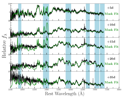
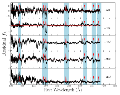
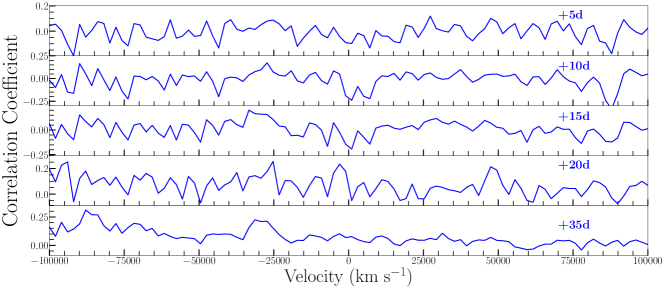
Figure 21: SN 2005cc. Phase relative to B band maximum.

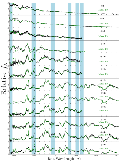
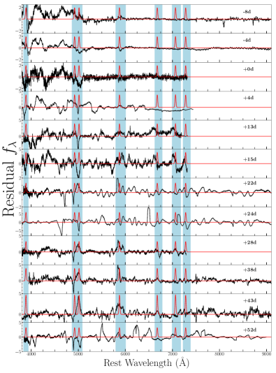
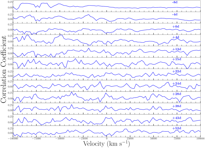
Figure 22: SN 2005hk. Phase relative to B band maximum.

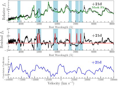
Figure 23: SN 2006hn. Phase relative to B band maximum.

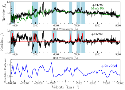
Figure 24: SN 2007ie. Phase relative to B band maximum and calculated using SNID.

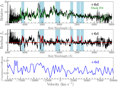
Figure 25: SN 2007qd. Phase relative to B band maximum.

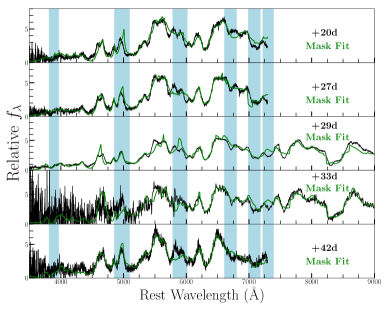
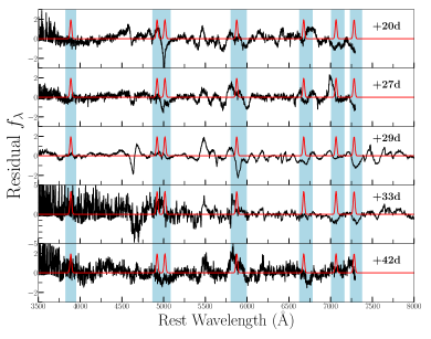
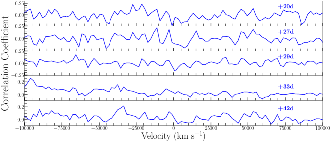
Figure 26: SN 2008A. Phase relative to B band maximum.

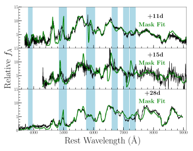
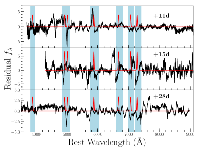
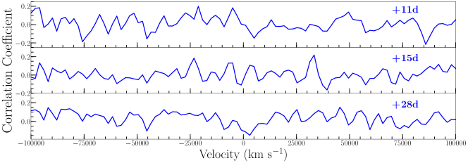
Figure 27: SN 2008ae. Phase relative to B band maximum.

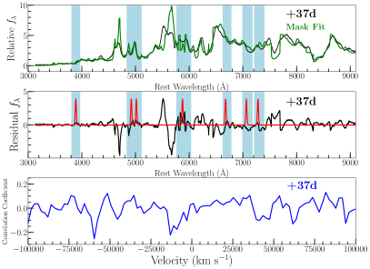
Figure 28: SN 2008ge. Phase relative to B band maximum.

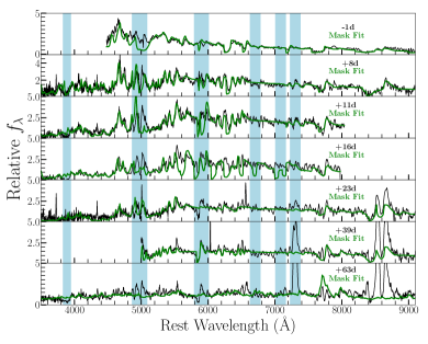
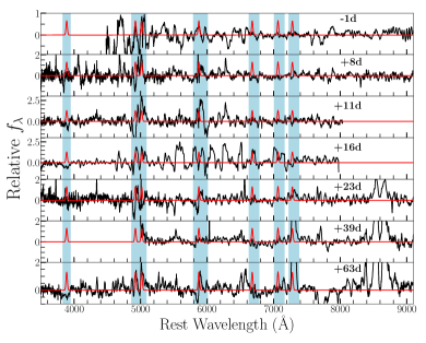
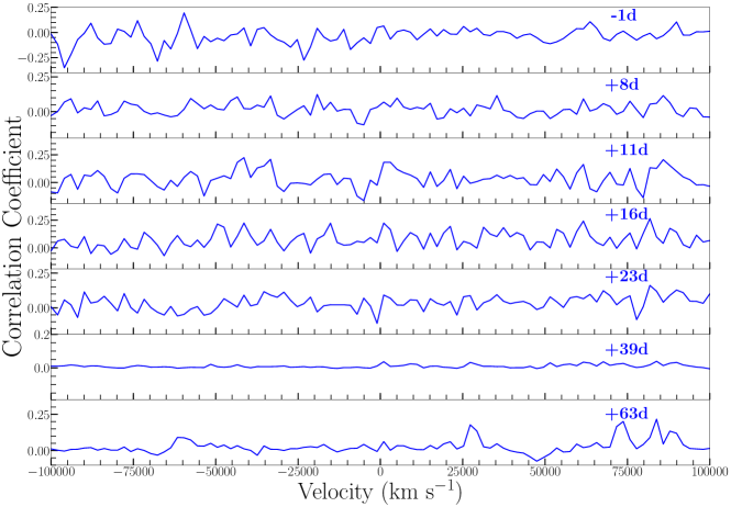
Figure 29: SN 2008ha. Phase relative to B band maximum.

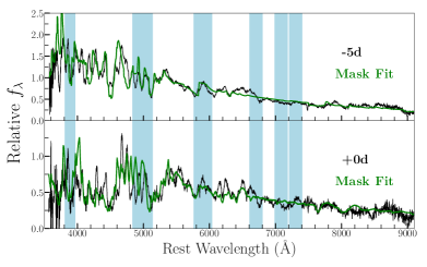
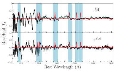
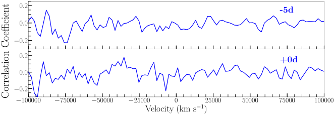
Figure 30: SN 2009J. Phase relative to B band maximum.

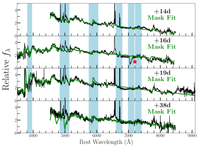
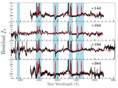
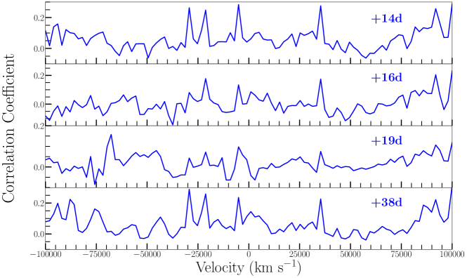
Figure 31: SN 2009ku. Phase relative to B band maximum. Red star indicates telluric absorption.

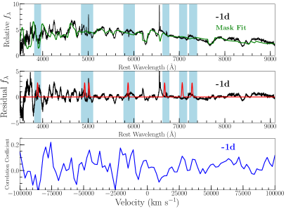
Figure 32: SN 2010ae. Phase relative to B band maximum.

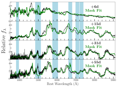
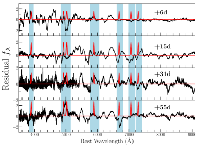
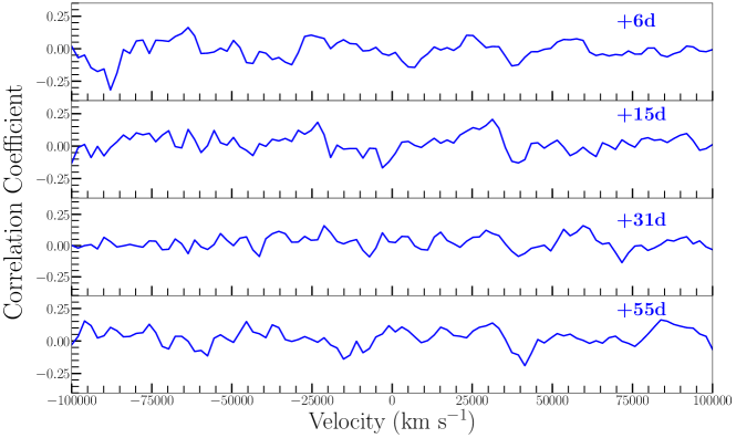
Figure 33: SN 2011ay. Phase relative to B band maximum.

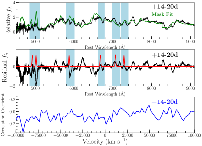
Figure 34: SN 2011ce. Phase relative to B band maximum and calculated using SNID.

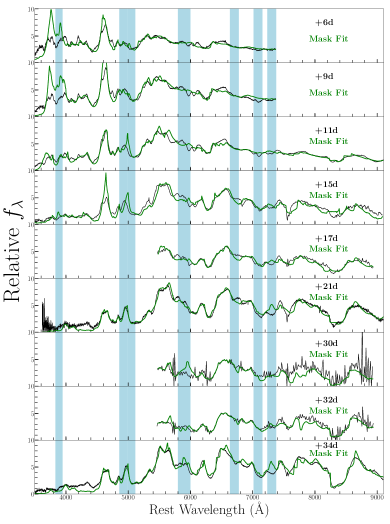
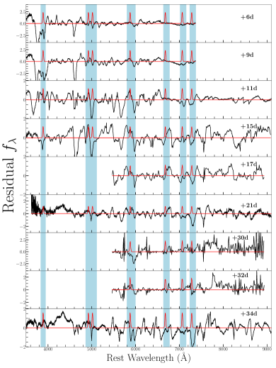
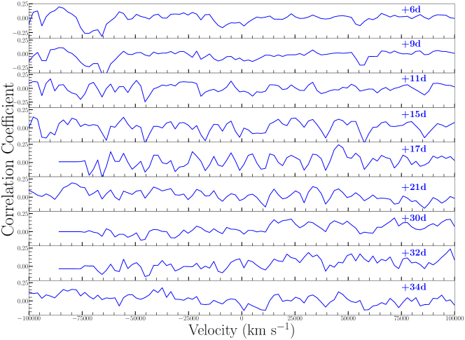
Figure 35: SN 2012Z. Phase relative to B band maximum.

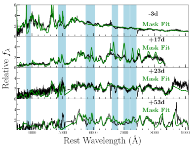
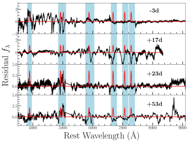
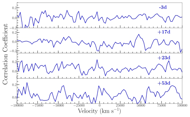
Figure 36: PS1-12bwh. Phase relative to B band maximum.

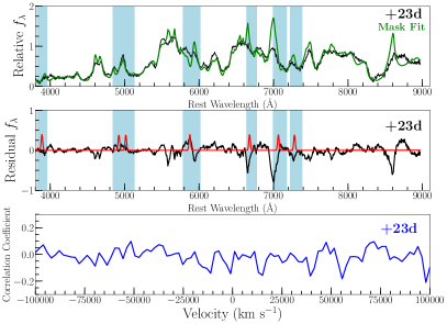
Figure 37: LSQ12fhs. Phase relative to B band maximum.

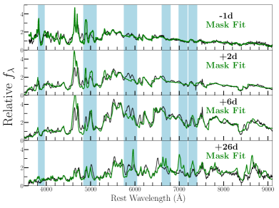
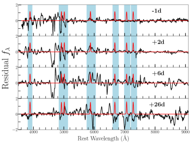
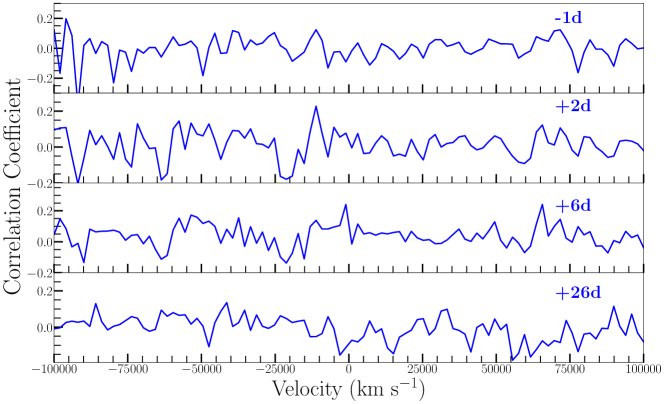
Figure 46: SN 2015H. Phase relative to B band maximum.

We now turn to fitting all available early-time SN Iax spectra to determine if any have He i emission. Since the helium features in the SNe 2004cs and 2007J spectra have Gaussian line profiles, we assume that features in other spectra would be similar. To properly fit for these features, we mask out regions around each prominent He i emission line and only fit the portions of the spectrum without potential He i emission. The wavelength ranges that are applied as masks in each fit are shown in blue in Figure 5. Each given fit to the data with masked out regions are plotted as green lines in Figures 17-46.

Once our spectral models are complete, we subtract the mask fit spectrum from the data and examine the residuals in each wavelength region where helium emission is known to occur. We then perform a visual inspection of each residual spectrum for obvious helium emission lines. Because pure emission lines can be represented as Gaussian profiles centered at a given central wavelength, we also cross-correlate the data residuals with a set of Gaussians (all with the same height and a superficial FWHM of 20 Å to prevent overlap of He i lines) centered at the rest wavelength of prominent optical He i lines: 3888.65, 4921.93, 5015.68, 5875.63, 6678.15, 7065.19, and 7281.35 Å. We cross-correlate by shifting the Gaussians for range of velocities. While the height and width of each Gaussian affects the specific correlation coefficient, these choices do not impact the relative correlation coefficient for a range of velocities. Furthermore, we tested the effect of binning on each analyzed spectrum and find that it does not impact the relative correlation coefficient. Examples of prominent residual emission in SNe 2004cs and 2007J are shown in Figures 5 and 8, respectively.

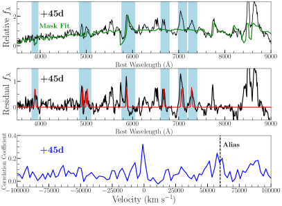
Figure 5: Top: SYNAPPS fit to SN 2004cs spectral data at +45d. Phase relative to clear band maximum. Blue regions are masked out in fit shown in green. Middle: In black, residuals of data and mask fit. In red, Gaussian profiles centered at prominent He i emission lines. Bottom: Cross correlation of Gaussian profiles and residual flux. Alias correlations marked by dashed black lines at $60$,000 $\textrm{km}\,\textrm{s}^{-1}$.

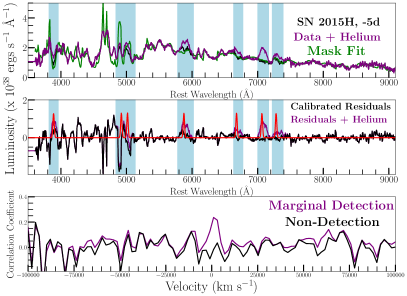
Figure 6: Top: In black, calibrated spectrum of SN 2015H at -5d with SYNAPPS mask fit shown in green. In purple, calibrated spectrum with He i lines from SN 2007J added in. Middle: In black, residuals of SN 2015H and mask fit. In purple, residuals of mask fit and SN 2015H plus He i lines. In red, Gaussian profiles centered at prominent He i emission lines. Bottom: Cross correlation of Gaussian profiles and residual luminosity for original spectrum (black) and spectrum with helium added (purple). Purple line shows a positive detection of helium.

To determine if a spectrum has a significant detection of helium emission, we cross-correlate all residual spectra with the helium line Gaussian profiles described above. We use a window of ${\pm}10^{6}$ $\textrm{km}\,\textrm{s}^{-1}$, which is much larger than physically possible for helium lines, to estimate the false-detection level. We define a significant detection if the correlation coefficient function has its global maximum within 1000 $\textrm{km}\,\textrm{s}^{-1}$ of zero velocity. The numerical peak in the correlation coefficient function is variable between spectra and thus needs to be analyzed on a case-by-case basis once a visually significant peak is detected with the cross-correlation. At certain velocities that correspond to distinct velocity shifts between the He i lines, there can be a large correlation coefficient. We examine these aliased peaks in detail, and if there is both a peak near zero velocity and at an aliased velocity, we examine the spectrum in more detail.

Using this method, we robustly detect He i features in the $+9-22$, $+33-46$, and $+65-78$-day spectra of SN 2007J (Figure 8c) and the single +45-day spectrum of SN 2004cs (Figure 5).

For the $+9-22$-day spectrum, there is a positive correlation peak around $-90$,000 $\textrm{km}\,\textrm{s}^{-1}$ (marked by a dashed line in Figure 8c) that is similar in strength to the peak near zero velocity. This correlation is caused by aliasing between the different helium lines (as well as other features in the residual spectrum). Examining the spectrum in detail, there is clear emission corresponding to the He i 6678.15 and 7065.19 lines. We therefore consider the main peak at zero velocity to be genuine and the detection of He i to be significant.

For the $+5-18$-day SN 2007J spectrum, we do not detect He i features by either visually inspecting the residual spectrum or by examining the correlation coefficients. Filippenko et al. (2007) first saw the increasing helium emission with phase.

Examining all additional early-time spectra, we do not detect any helium lines for any of the additional 42 SNe Iax examined. We present the all spectra and accompanying fits in Appendix A.

Since these spectra do not have any detected He i lines, we estimate the luminosity limit for these features. To do this, we first scale the flux in each spectrum to match the corresponding broad-band photometry as determined by images, and then add helium features until the features can be detected in each spectrum. To do this, we add the $33-46$-day SN 2007J residual spectrum, which has particularly high signal-to-noise ratio He i features, to each spectrum. This residual spectrum has the flux at all wavelengths other than those coincident with the He i features set to zero and is a representative helium emission spectrum for SNe Iax. Each spectrum’s original continuum and features remain unchanged when this helium emission spectrum is added. We note, however, that this specific helium residual spectrum from SN 2007J is not ideal for such a method due to its difference in phase from other SNe Iax in the sample. However, because these differences would at most make the helium more difficult to detect, the $33-46$-day residual spectrum of SN 2007J is a conservative upper limit for helium detection in other objects.

Once the helium residuals are added, we then scale the flux of the SN 2007J residual spectrum until the features are detected, and record the corresponding line flux as the detection limit. Same as the true detections in SNe 2004cs and 2007J, a detection here is also defined as a peak in the correlation coefficient function within 1000 $\textrm{km}\,\textrm{s}^{-1}$ of zero velocity. An example of this calculation for a marginal detection (i.e. same as $+9-22$d detection in SN 2007J) of helium is shown for SN 2015H in Figure 6. The luminosity limits for helium detection in the 6678.15 Å line are shown in Figure 7. Since we use a single spectrum to determine the luminosity limits, limits for all lines are perfectly correlated. The lines have scaling factors of L_λ5876 = 1.47 $\cdot$ L_λ6678 and L_λ7065 = 2.33 $\cdot$ L_λ6678.

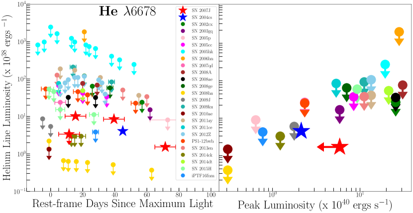
Figure 7: Left: Luminosity limits needed for detection of $6678$Å helium line. All SNe Iax shown are flux calibrated. True detections in SNe 2004cs and 2007J are shown as blue and red stars, respectively. Right: Most constraining luminosity limits of $6678$Å line with respect to peak luminosity.

As seen in Figure 7, SNe 2004cs and 2007J have detected helium at a luminosity significantly below the limits for most SNe Iax in our sample. Additionally, as seen for SN 2007J, the helium luminosity is expected to vary with phase. Combined, we can use the detection luminosity as a function of phase to define an envelope where we would expect to detect helium features similar to those seen in SNe 2004cs and 2007J. Of the 23 SNe Iax examined, 17 do not have sufficiently deep limits to rule out helium features as luminous as the SN 2004cs and 2007J features. As such, conclusions drawn from those SNe are limited.

However, 4 SNe Iax, SNe 2008ha, 2014ck, 2015H and iPTF16fnm, have spectra over the appropriate phase range and with limits as deep or deeper than the He i luminosity detections for SNe 2004cs and 2007J. Therefore these 6 SNe Iax represent the sample of SNe Iax where we can directly compare to known detections. The spectra of SNe 2008ha, 2014ck and 2015H at phases near $\sim 22$ days are presented in Figure 9 for comparison to the $9-22$-day epoch of SN 2007J.

In Figure 7, we compare the He i $\lambda$6678 luminosity to the SN Iax peak luminosity Jha (2017, and references therein). There is a general trend between the peak luminosity and the He i luminosity limit. This is primarily driven by the signal-to-noise ratio of the spectra (which is usually similar for all spectra) and the ability for SYNAPPS to accurately reproduce a spectrum.

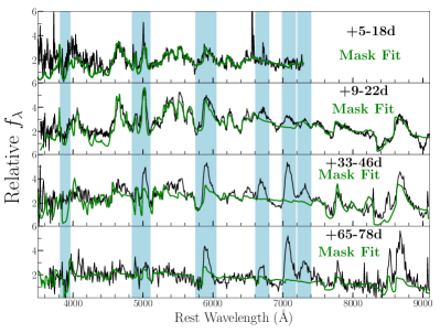
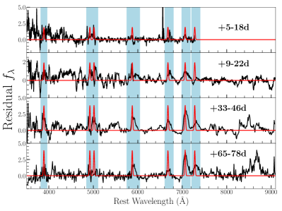
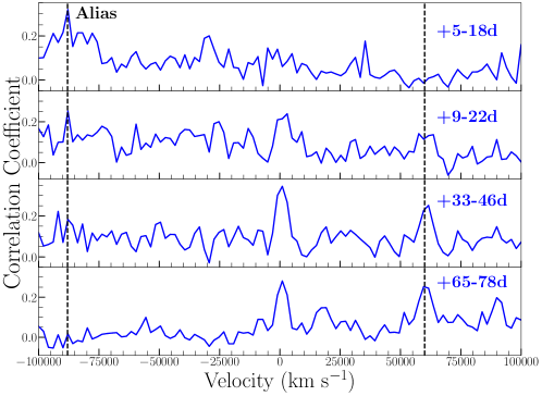
Figure 8: (a) SYNAPPS fits to SN 2007J spectral data at $+5-18$, $+9-22$, $+33-46$ and $+65-78$d. Phase relative to clear band maximum. Blue regions are masked out in fit shown in green. (b) In black, residuals of data and mask fit. In red, Gaussian profiles centered at prominent He i emission lines. (c) Cross correlation of Gaussian profiles and residual flux. Alias correlations marked by dashed black lines at $-88$,000 $\&$ $60$,000 $\textrm{km}\,\textrm{s}^{-1}$.

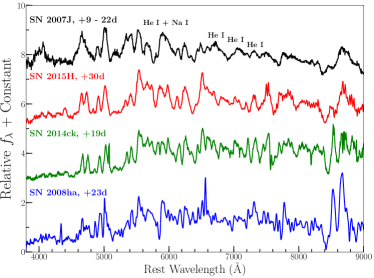
Figure 9: Spectral comparison of SN 2007J, SN 2008ha, SN 2014ck and SN 2015H at approximately the same phase. The spectra are ordered by decreasing He i luminosity limits.

4 Search for Late-time Emission Features

In single-degenerate (SD) progenitor models for SNe Ia, we expect the SN to sweep up material ablated from a close companion star and/or in the circumstellar environment. This material should emit and be detectable in late-time spectra as narrow emission lines (Marietta et al., 2000; Mattila et al., 2005; Liu et al., 2010; Liu et al., 2012, 2013a; Pan et al., 2012; Lundqvist et al., 2013). While there have been no detected hydrogen or helium emission lines in any late-time SN Ia spectrum (e.g., Mattila et al., 2005; Leonard, 2007; Shappee et al., 2013; Lundqvist et al., 2013; Maguire et al., 2016; Graham et al., 2017; Sand et al., 2018; Shappee et al., 2018; Dimitriadis et al., 2018), we attempt to calculate upper limits for the amount of stripped hydrogen and helium mass present in SNe Iax late-time spectra.

Upon visual inspection of all late-time SN Iax spectra, we find no obvious hydrogen or helium narrow-line emission. As in Lundqvist et al. (2015), we also examine each late-time spectra for Ca ii and O i emission but find no visual detections.

Below, we provide quantitative mass limits on swept-up hydrogen and helium material.

4.1 Stripped Hydrogen in Late-time Spectra

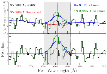
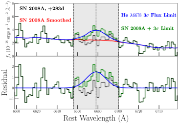
Figure 10: (a) Top: In black, flux calibrated late-time data of SN 2008A at +283d with no apparent H-$\alpha$ emission. Shown in red is the smoothed continuum with the $3\sigma$ RMS flux limit for marginal detection of H-$\alpha$ shown in blue. Data plus $3\sigma$ flux limit shown in green. Grey shaded region represents a wavelength range of 22Å ($\sim 1000$ km s^-1). Bottom: In green, residuals of data plus the $3\sigma$ limit and smoothed data. In black, residuals of data and smoothed continuum. H-$\alpha$ $3\sigma$ flux limit shown in blue. (b) Same method as for H$\alpha$, but with marginal detection of $6678$Å He i emission line.

To determine the line luminosity limit for each spectrum, we employ the same method as Sand et al. (2018). By representing the H-$\alpha$ emission lines as Gaussian profiles, we calculate the flux limit needed for marginal detection. As in Sand et al. (2018), we estimate the peak flux of the emission line to be three times the spectrum’s root-mean-square (RMS) flux, with the spectral feature having a FWHM of 1000 $\textrm{km}\,\textrm{s}^{-1}$. From our 3-$\sigma$ flux limit, we calculate a luminosity limit for marginal detection of an H-$\alpha$ emission line. An example of simulated marginal detection of H-$\alpha$ is shown in Figure 10(a) for SN 2008A at a phase of +281 days. We present the H-$\alpha$ luminosity limits as a function phase for all SNe Iax with late-time spectra in Figure 11(a).

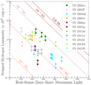
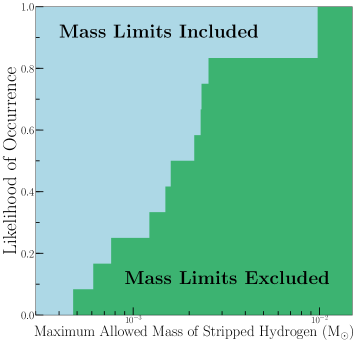
Figure 11: (a) Luminosity limits for marginal detection of hydrogen emission in late-time SN Iax spectra. Contours are stripped masses calculated using Equation 1 with an exponential time-dependence of SNe Iax at late-times. (b) Cumulative distribution of converted hydrogen luminosity limits into masses using Equation 1. Blue portion represents included stripped mass limits for hydrogen while green portion holds excluded limits.

We then use the Botyánszki et al. (2018) relation to convert the luminosity limits into stripped-mass limits,

$$\log_{10}(L_{\rm{H\alpha}})=-0.2M_{1}^{2}+0.17M_{1}+40,$$ (1)

where $L_{\rm{H\alpha}}$ is the H-$\alpha$ luminosity in cgs units at 200 days after peak, $M_{1}=\log_{10}(M_{\rm H}/M_{\odot})$, and $M_{\rm H}$ is the stripped hydrogen mass. Since this relation is only valid at 200 days after peak, we scale the luminosity limits to that epoch, assuming an exponential decline seen for SNe Iax (Stritzinger et al., 2015). We fit this exponential to the observed late-time luminosities of SNe 2005hnk and 2012Z (see Figure 8 of Stritzinger et al. 2015) and apply this function to other SNe Iax in order to calculate line luminosities at 200 days. For each SN, we determine the most-constraining mass limit. We display the cumulative distribution of mass limits in Figure 11(b).

It should be noted that the models presented in Botyánszki et al. (2018) are designed for SNe Ia and not explicitly for SNe Iax. Thus these models are most notably different than SNe Iax in their energetics, explosion asymmetry and total Ni mass produced. As a result, the SN ejecta density and the mixing of H or He may be impacted by the lower explosion energies in SNe Iax, but the differences in Ni mass between the two explosion types will scale directly with the luminosity. Additionally, any potential explosion asymmetry is seemingly negligible given the current consistency in polarization between SNe Iax and SNe Ia (Chornock et al., 2006; Maund et al., 2010). Nevertheless, the relation derived in Botyánszki et al. (2018) from radiative transfer simulations is currently the most applicable model for this analysis if we assume that SNe Iax arise from a SD scenario where the impact of the SN ejecta with the companion star results in stripped or swept up H- or He-rich material.

For our late-time SN Iax sample, the mass limits range from $5\times 10^{-4}$ to $1\times 10^{-2}\ {\rm M}_{\odot}$ with a typical limit of $2\times 10^{-3}\ {\rm M}_{\odot}$. This is about an order of magnitude larger than that expected for the amount of stripped hydrogen expected to be swept-up by a SN Ia in a Roche-lobe filling progenitor system ($1.4\times 10^{-2}$ to $0.25\ {\rm M}_{\odot}$; Pan et al., 2012; Liu et al., 2012; Boehner et al., 2017). Liu et al. (2013b) estimates that a SN Iax with a similar progenitor system would have $1\times 10^{-2}-1.6\times 10^{-2}\ {\rm M}_{\odot}$ of stripped hydrogen, also significantly higher than the limits for our sample.

4.2 Stripped Helium in Late-time Spectra

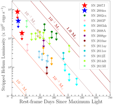
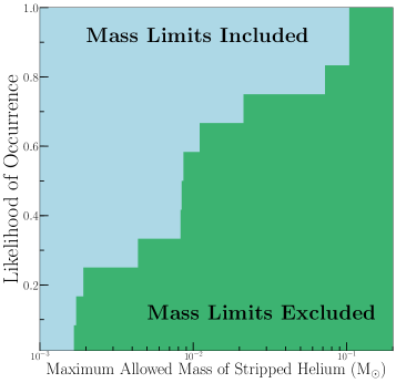
Figure 12: (a) Luminosity limits for marginal detection of helium emission in late-time SN Iax spectra. Contours are stripped masses calculated using Equation 2 with an exponential time-dependence of SNe Iax at late-times. Red and blue stars are the early-time detections of helium and the luminosities of the He $\lambda 6678$ line. These are shown as upper limits because the are not true detections of late-time, stripped helium, and are placed for reference to late-time flux limits for marginal detection of stripped helium. (b) Cumulative distribution of converted helium luminosity limits into masses using Equation 2. Blue portion represents included stripped mass limits for helium while green portion holds excluded limits.

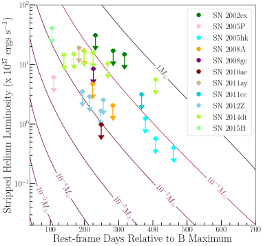
Figure 13: Luminosity upper limits for marginal detection of helium emission in late-time SN Iax spectra. Contours are stripped masses calculated using Equation 12. Masses are calculated with a velocity of 5000 km s^-1 and $M_{\rm Ni}=0.1{\rm M}_{\odot}$.

We also examine all late-time SN Iax spectra for helium emission that could result from companion interaction. Upon visual inspection, we find no detections of any prominent He i emission lines. Following the same method as described in Section 4.1, we calculate luminosity limits for the He i $\lambda$6678 line. An example of the calculation of the 3-$\sigma$ limit for SN 2008A is shown in Figure 10(b).

Using Equation 1, Sand et al. (2018) equates H-$\alpha$ emission to He i emission to calculate the upper limit of helium emission in the late-time spectra of SN 2017cbv (i.e., $L_{\rm{H\alpha}}=L_{\rm{He}}$). We use a similar method but scale the input helium luminosity based on the relative luminosities of H-$\alpha$ and He i emission found by Botyánszki et al. (2018). To do this, we compare the H-$\alpha$ line luminosity in Figure 1 of Botyánszki et al. (2018) to the He i $\lambda$6678 line luminosity shown in their Figure 4 for the MS38 model. Based on the relative peaks and FWHM of each respective emission line, the MS38 model produces an H-$\alpha$ emission line that is ${\sim}5$ times more luminous than the He i $\lambda$6678 emission line for the same mass. As a result, we use

$$\log_{10}(L_{\rm{He}})=-0.2M_{1}^{2}+0.17M_{1}+39.3,$$ (2)

where $M_{1}=\log_{10}(M_{\rm He}/M_{\odot})$, and $M_{\rm He}$ is the stripped helium mass, to calculate the amount of stripped helium in SNe Iax. This estimate comes with significant caveats. The efficiency of non-thermal excitation of He is dependent on the degree of Ni mixing in the SN ejecta (Lucy, 1991). This poses a significant challenge for this type of modeling, as it means that the strength of the He lines is dependent on the distribution of the Ni within the explosion itself and the distribution of the entrained He within the ejecta. This illustrates the potential limitations of the application of the Botyánszki et al. (2018) result to SN Iax with He-rich companions: the Ni distribution is from a Ia-like explosion and the He distribution comes from a simulation of interaction with an H-rich companion, but with the entrained H artificially converted to He. However, Botyánszki et al. (2018) is at present the most applicable model available in the literature.

We display the helium luminosity limits for our SN Iax sample as a function of phase and compare to expected helium line luminosity for various amounts of stripped helium in Figure 12(a). We also plot a cumulative distribution of calculated helium masses, using the most constraining value for each SN, in Figure 12(b). For reference, we add the early-time He $\lambda$6678 luminosities for SNe 2004cs and 2007J as upper limits in Figure 12(a). Without a method for converting early-time helium luminosity to mass, these points represent upper limits on the amount stripped helium that could be visible at early-times if we assume that the helium detected in SNe 2004cs and 2007J is the result of companion interaction. Nonetheless, we caution the use of these specific limits in constraining companion interaction models because the photospheric heating mechanism and specific excitation energy of helium in SNe Iax is still unclear at this time.

For our SN Iax sample, we find a range of stripped helium upper limits of $2\times 10^{-3}$ to $1\times 10^{-1}\ {\rm M}_{\odot}$. Comparing these stripped helium mass limits to those predicted by SN Ia explosion models, we find that some of our limits are consistent with predicted stripped masses, but the most constraining limit of $2\times 10^{-3}\ {\rm M}_{\odot}$ is lower than that presented in companion interaction models. For stripped helium, Pan et al. (2012) predicts a range of $2.45\times 10^{-3}-1.34\times 10^{-2}\ {\rm M}_{\odot}$ and Liu et al. (2013a) predicts a range of $9.5\times 10^{-3}-2.8\times 10^{-2}\ {\rm M}_{\odot}$.

In addition to using a (modified) relation between line flux and stripped mass determined by simulations (Botyánszki et al., 2018), we present an alternate, analytic method of calculating stripped helium mass, derived from radioactive-decay powered SN ejecta. We first assume that the helium is contained in a homogeneous shell about the SN with mass $M_{\rm He}$ and a radius $\Delta r$ that is changing with the expanding ejecta. The shell’s density can then be defined as:

$$\rho=\frac{M_{\rm He}}{4\pi r^{2}\Delta r}.$$ (3)

The optical depth of $\gamma$-rays from radioactive decay in SNe is

$$\tau_{\gamma}=\kappa\rho\Delta r,$$ (4)

where $\kappa=0.05$ cm² g^-1 is used for $\gamma$-rays.

Combining Equations 3 and 4, we find a relation for optical depth of $\gamma$-rays as a function of $M_{\rm He}$:

$$\tau_{\gamma}=\frac{\kappa M_{\rm He}}{4\pi r^{2}}.$$ (5)

We define the luminosity absorbed by the helium shell to be:

$$L_{\rm dep}=L_{\rm rad}\left(1-e^{-\tau_{\gamma}}\right),$$ (6)

where $L_{\rm rad}$ is the luminosity of radioactive ⁵⁶Ni and ⁵⁶Co. We assume that the ejecta is optically thin to gamma-rays and thus does not get absorbed in the ⁵⁶Ni region before reaching the helium shell. The $L_{\rm rad}$ relation is from Equation 19 of Nadyozhin (1994),

$$L_{\rm rad}=1.45\times 10^{43}\left[4.45\cdot e^{-(t/8.8\rm{~{}d})}+e^{-(t/111.3\rm{~{}d})}\right]\frac{M_{\rm Ni}}{{\rm M}_{\odot}}.$$ (7)

We define the helium line luminosity to some fraction of the deposited helium energy,

$$L_{\textrm{dep,He}}=\frac{L_{\textrm{He,line}}}{f},$$ (8)

where $f$ is the fraction of deposited energy emerging in the helium line. There are $\approx 10$ He i lines in the optical. With the conservative assumption that the helium luminosity is equally distributed across these lines, we adopt a rough estimate of $f=0.1$. Combining Equations 5, 6 and 8, we find

$$L_{\textrm{dep,He}}=L_{\rm rad}\left(1-e^{-\frac{\kappa M_{\rm He}}{4\pi r^{2}}}\right).$$ (9)

Solving for $M_{\rm He}$ and replacing the radius, $r$, with the product of ejecta velocity and time since explosion, we have

$$M_{\rm He}=-\frac{4\pi(vt)^{2}}{\kappa}\ln\left[1-\left(\frac{L_{\textrm{He,line}}}{L_{\rm rad}}f^{-1}\right)\right]{\rm M}_{\odot}$$ (10)

Picking nominal values for each quantity and assuming that ⁵⁶Co decay dominates the energy deposition at the epochs of interest, we find

$$\begin{aligned} &M_{\rm He}=-2.35\,\mathrm{{\rm M}_{\odot}}\left(\frac{v}{5000\,\mathrm{\textrm{km}\,\textrm{s}^{-1}}}\right)^{2}\left(\frac{t}{100\,\mathrm{d}}\right)^{2}\left(\frac{\kappa}{0.05\,\mathrm{cm^{2}\,g^{-1}}}\right)^{-1}\times\\ &\ln\left[1-6.9\times 10^{-4}\left(\frac{f}{0.1}\right)^{-1}\left(\frac{L_{\rm He}}{10^{38}\,\mathrm{erg\,s^{-1}}}\right)\left(\frac{M_{\rm Ni}}{0.1\,\mathrm{{\rm M}_{\odot}}}\right)^{-1}\exp\left(\frac{t/100\,\mathrm{d}}{1.113}\right)\right]\end{aligned}$$ (11)

Because the quantity in the square brackets is approximately one, we can Taylor expand the natural logarithm to find a final expression for $M_{\rm He}$,

$$\begin{aligned} &M_{\rm He}=1.6\times 10^{-3}\,\mathrm{{\rm M}_{\odot}}\left(\frac{v}{5000\,\mathrm{\textrm{km}\,\textrm{s}^{-1}}}\right)^{2}\left(\frac{t}{100\,\mathrm{d}}\right)^{2}\left(\frac{\kappa}{0.05\,\mathrm{cm^{2}\,g^{-1}}}\right)^{-1}\times\\ &\left(\frac{f}{0.1}\right)^{-1}\left(\frac{L_{\rm He}}{10^{38}\,\mathrm{erg\,s^{-1}}}\right)\left(\frac{M_{\rm Ni}}{0.1\,\mathrm{{\rm M}_{\odot}}}\right)^{-1}\exp\left(\frac{t/100\,\mathrm{d}}{1.113}\right)\end{aligned}$$ (12)

We note that Equation 12 yields a reasonable mass estimate for the nominal values. However, if one requires estimates far from the nominal values, Equation 11 may be more appropriate.

In Figure 13, we plot the stripped helium luminosity limits as a function of phase for our late-time SN Iax sample. For comparison, we also display lines of equal stripped helium mass as derived with Equation 12 and assuming an ejecta velocity of 5000 $\textrm{km}\,\textrm{s}^{-1}$ and a ⁵⁶Ni mass of $0.1\ {\rm M}_{\odot}$. However, these are average values based on the known range of ejecta velocities and ⁵⁶Ni masses in SNe Iax (Foley et al., 2013; Stritzinger et al., 2015; Jha, 2017). We note that Figure 13 is illustrative and makes various assumptions about the physical conditions of the system. Consequently, we suggest calculating $M_{\rm He}$ from Equation 12 with values for ejecta velocity and $M_{\rm Ni}$ specific to a given SN Iax. Under those assumptions, we can place stripped helium mass limits of $\sim{}3\times 10^{-3}-7\times 10^{-1}\ {\rm M}_{\odot}$, comparable to the values derived from the numerical simulations above.

5 Discussion

5.1 Rate of Helium Detection in SNe Iax

We have modeled the early-time spectra of 44 classified SNe Iax and find prominent helium emission in the spectra of only two objects, SNe 2004cs and 2007J. In order to understand this observational result, we must account for selection effects. In particular, the luminosity of the detected helium lines was significantly lower than the limits for the majority of the sample; 19/25 objects ($76\%$) do not have deep enough limits to detect lines as faint as in SNe 2004cs and 2007J. Furthermore, we could not significantly detect helium in the first spectrum of SN 2007J, despite there being very strong lines in its later spectra. Therefore, temporal evolution is also likely important for determining the detectability of helium for our sample.

Using the subset of SNe Ia where we could detect helium lines with a similar luminosity as for SNe 2004cs and 2007J, we see that 2/6 ($33^{+11}_{-7}$%) SNe Iax have helium detections. Any SN Iax model must allow for similar fractions of SNe where helium is and is not observable in their spectra. We examine some of the possible physical models below.

5.2 Explanations for Helium in the SN Iax System

We find that the helium profiles in SNe 2004cs and 2007J are inconsistent with P-Cygni profiles and are well described by a Gaussian profile. This indicates that the helium is not in the photosphere, and instead in the circumstellar environment. We find that the He i $\lambda$7065 line in SN 2007J has a FWHM of 4352 and 4725 $\textrm{km}\,\textrm{s}^{-1}$ at $+33-46$ and $+65-78$ days, respectively. The same line has a FWHM of 3878 $\textrm{km}\,\textrm{s}^{-1}$ for SN 2004cs at a phase of +45 days. Additionally, there is He-rich material at velocities as high as 8367 $\textrm{km}\,\textrm{s}^{-1}$ (with the lines having a full-width zero intensity of ${\sim}$12,000 $\textrm{km}\,\textrm{s}^{-1}$). These velocities are higher than the orbital motion and escape velocity of the system, indicating that an explosive mechanism is necessary to eject helium into the SN Iax progenitor system.

In the WD+He star channel for SNe Iax progenitors, the accretion rate of helium onto the surface of the C/O WD modulates the amount of He-rich material in the circumstellar environment. If the accretion rate is low ($\dot{M}<10^{-6}\ {\rm M}_{\odot}$yr^-1), it can lead to helium flashes (e.g., Piersanti et al., 2014; Brooks et al., 2016) resulting in helium novae. A possible explanation for the small fraction of SNe Iax with helium detections could be the occurrence of such pre-explosion helium nova eruptions. In the C/O WD + He star progenitor system, the helium mass transfer rate from the He star onto the WD varies based on the size of the non-degenerate companion. Through modeling of these systems for an initial $1\ {\rm M}_{\odot}$ WD, Brooks et al. (2016) show that systems with lower mass companion stars also experience lower mass transfer rates prior to explosion. Consequently, systems with 1.3–$1.4\ {\rm M}_{\odot}$ He stars undergo helium nova eruptions as the WD approaches the Chandrasekhar mass (see Figure 3 of Brooks et al. 2016). Occurring in only a fraction of such scenarios, these nova eruptions would enrich the progenitor system with helium in the final years before explosion. However, the ejected He-rich material may be hidden in cavities of the progenitor system (Wood-Vasey & Sokoloski, 2006) and could lead to an even lower rate of helium detection.

Higher-mass He star companions have higher mass transfer rates, allowing for steady helium burning on the WD surface and does not produce helium flashes. For these high accretion rates, a super-Eddington wind may be formed, which will remove accreted helium from the system thus making it undetectable (Wang et al., 2015). Consequently, the limited fraction of C/O WD + He star systems with helium novae could explain the detection of helium emission in only the spectra of SNe 2004cs and 2007J.

Interestingly, the single Galactic helium nova, V445 Puppis, has helium at velocities as high as 6000 $\textrm{km}\,\textrm{s}^{-1}$ (Woudt et al., 2009), consistent with the helium velocity seen for SNe 2004cs and 2007J.

5.3 Photospheric Helium Models

Using a TARDIS model with significant photospheric helium, Magee et al. (2019) are able to fit the prominent He i features in the +9-22d spectrum of SN 2007J. However, as shown in Figure 2, we also reproduce all He i features by using a masked SYNAPPS fit with added helium Gaussian profiles. This indicates that while the interpretation of Magee et al. (2019) may be correct, our model of circumstellar helium in SN 2007J is not obviously ruled out. However, all later SN 2007J spectra have clear Gaussian He i line profiles and thus cannot have a photospheric origin. This is not necessarily at odds with the Magee et al. (2019) result, but it should be noted that they do not attempt to fit these later spectra of SN 2007J nor the SN 2004cs spectrum. Nonetheless, it is possible that there exists both photospheric and circumstellar helium in SNe Iax; this being consistent with both results as well as having a dependence on the quantity of helium at a given location within the SN.

5.4 Comparison to Single-Degenerate Explosion Models

The leading model for the SN Iax progenitor system is a WD accreting mass from a non-degenerate He star companion. Based on the calculated fraction of SNe Iax with helium, the companion to the WD could also be another type of non-degenerate star such as a Main Sequence, Red Giant, or He star. Support for the He-star scenario comes from the pre-explosion observation of the SN 2012Z progenitor system, which is consistent with a He-star companion despite the lack of helium lines in its spectra (McCully et al. 2014; Takaro et al. 2019; McCully et al., in prep).

Even for the WD+He star progenitor channel, there are a variety of explosive mechanisms that could trigger a SN Iax explosion as the He star fills its Roche Lobe and transfers matter onto the WD. The typical Chandrasekhar-mass model involves accretion of He-rich material and steady burning on the WD surface until the WD reaches M${}_{\textrm{ch}}$ and explodes. The detection of strong Ni features in the late-time spectra of SNe Ia indicate a high central density for the WD, consistent with a M${}_{\textrm{ch}}$ explosion (Stritzinger et al., 2015; Foley et al., 2016).

Alternatively, a sub-Chandrasekhar mass model with helium detonation on the surface of the WD may be more appropriate in describing these objects (Hillebrandt & Niemeyer, 2000). Wang et al. (2013) examines this double-detonation model for SNe Iax and finds that such a scenario reproduces the observed $M_{V,{\rm~{}peak}}$ for these objects, as well as allows for SNe with helium lines in their spectra as in SNe 2004cs and 2007J. This type of explosion in the WD+He star progenitor channel could explain the lowest luminosity SNe Iax such as SNe 2008ha and 2010ae, but ultimately cannot reproduce the low ejecta velocities seen in all SNe Iax. As stated above, the Nickel abundances found in late-time SN Iax spectra by Foley et al. (2016) indicates that the majority of SNe Iax are the result of M${}_{\textrm{ch}}$ explosions rather than sub-Chandrasekhar mass explosions.

In each explosion model discussed, the type of helium burning may also affect the detection of helium within SNe Iax. The lack of helium in most SNe Iax spectra can be explained by an explosion that completely burns the surface helium. Complete burning may generate a more luminous explosion that could result in a lack of detected helium in the most-luminous SNe Iax. Within the limits of detection, the presence of detectable helium in 33% of SNe Iax could be explained by incomplete burning where unburned helium remained in a fraction of systems after explosion.

The SD channel, such as a WD+He star progenitor system, has also been examined in the context of companion interaction. In the pure deflagration explosion, the SN ejecta forms a shock wave that hits the companion He star and strips material from the stellar surface. As discussed in Sections 4.1 and 4.2, this material could be hydrogen or helium (depending on the composition of the companion star) and the amount of stripped mass depends on the exact explosion model and companion star. Hydrodynamical simulations done by Liu et al. (2013a) and Pan et al. (2012) show that the H- or He-rich material is removed due to ablation (SN heating) and mass stripping (momentum transfer). These models demonstrate that the impact of SN ejecta with the non-degenerate companion causes a hole in the ejecta of $\sim$$$ for the WD+He star system. While some of the stripped material will reside within this ejecta hole, the rest will be swept up by the expanding ejecta and may become visible as the SN luminosity fades at late-time.

However, we find no evidence of such material in the SN Iax late-time spectra despite the stripped mass predictions for H- and He-rich material from companion interaction. This indicates a discrepancy between SD model predictions and SN Iax (and SN Ia) observations, that perhaps could be reconciled by having “hidden” hydrogen/helium or a smaller amount of stripped material than predicted.

For SNe Iax in particular, Liu et al. (2013b) show that H-rich material can be hidden in late-time spectra due to the inefficient mass stripping ($<$0.01${\rm M}_{\odot}$). In their pure deflagration model, Liu et al. (2013b) demonstrate that the relatively low kinetic energy released in the explosion could result in both a low mass of stripped material and potentially no hydrogen emission signatures at late-times. Such a scenario is broadly consistent with the lack of hydrogen emission in late-time SNe Iax spectra, but the mass limit is still higher than those calculated in Section 4.1.

Another potential reason for a lack of visible helium emission is that the high excitation energy of helium may prevent the formation of the predicted narrow emission lines at late times. As is shown for Type Ic SNe, the degree of Ni mixing in the SN ejecta significantly influences the efficiency of non-thermal helium excitation (Lucy, 1991; Dessart et al., 2011, 2012). For SNe Iax, weak Ni mixing in the ejecta could result in helium lines below the limit of detection in late-time spectra.

Furthermore, the specific type of explosion responsible for SNe Iax could result in a lack of detectable stripped material from a companion star. The partial deflagration scenario in particular can produce a highly asymmetric explosion in which the ejecta either does not impact the companion at all, or causes much less impact than a spherical explosion (Jordan et al., 2012; Kromer et al., 2013; Fink et al., 2014). Such a scenario would strip less H- or He-rich material from the companion and would then produce material in the system below the limit of detection.

Finally, the strength of hydrogen or helium emission features may depend on the SN viewing angle and it could be the case that observed SNe Iax may have undetectable stripped material due to the angle of observation. We can match the detected occurence rate (33%) if He i features are only visible within a $71\mathrm{°}$ angle. This calculation assumes a spherically symmetric SN where circumstellar helium can only be detected on 33% of the SN ejecta.

Case in point, the ongoing discrepancy between SD interaction models and late-time observations warrants more robust radiative transport calculations through 3-D hydrodynamical stripping of hydrogen or helium from a companion star. The lack of visible hydrogen or helium emission at late-times highlights the need for SD models that can have both significant swept up or stripped mass and a lack of emission features at late-times. This could then explain the observed flux and mass limits that are well below those predicted by interaction models for SNe Ia and Iax.

With true detections of helium in SN Iax spectra, we have identified the need for luminosity-mass conversions in early-time spectra, not just in late-time phases. Such modeling would allow us to quantify the helium present in SN 2004cs, SN 2007J and potentially future SNe Iax with helium detections. Calculating the helium mass present at early-times will further constrain the proposed C/O WD + He star progenitor system for SNe Iax.

5.5 SD Scenario and SNe Ia

The pre-explosion detection of the progenitor system for SN 2012Z (McCully et al., 2014) strongly indicates a SD progenitor system for that SN, which by extension, may apply to other SNe Iax. Other observations indicating a short delay time (e.g., Foley et al., 2009; Lyman et al., 2013; Lyman et al., 2018), also favor a SD progenitor channel for SNe Iax. The specific scenario that best fits all observations is a near Chandrasekhar mass C/O WD primary with a Roche-lobe filling He-star companion (e.g., Foley et al., 2013; Jha, 2017).

A SN from such a system is expected to strip material from the companion star, possibly sweep up additional circumstellar material, and produce relatively narrow emission lines in late-time spectra (Liu et al., 2013a). However, we have not yet seen any such emission lines in our sample of 11 SNe Iax with late-time spectra. Moreover, we have not detected the “characteristic SD” narrow emission lines in SN 2012Z. Therefore, the lack of narrow emission lines in the late-time spectrum of a thermonuclear SN is poor evidence against the SD scenario. While it is currently unclear where the logical argument breaks down, there are significant implications for SNe Ia.

Several studies have searched for narrow emission lines in the late-time spectra of SNe Ia to see if there was evidence of interaction with a non-degenerate companion star, and thus far, no example has been found for a normal SN Ia (e.g., Mattila et al., 2005; Leonard, 2007; Shappee et al., 2013; Lundqvist et al., 2013; Maguire et al., 2016; Graham et al., 2017; Sand et al., 2018; Shappee et al., 2018; Dimitriadis et al., 2018, but see also Graham et al. 2018). While many of these studies concluded that the lack of such lines is strong evidence against (at least a subset of) SD scenarios for SNe Ia, our experience with SNe Iax suggests that such strong conclusions are premature.

We suggest a full re-evaluation to determine the utility of these observations for understanding the progenitor systems of SNe Iax and SNe Ia.

5.6 Future SN Iax Observations

As more SNe Iax are discovered, the number of objects with confirmed helium emission in their spectra should increase. Consequently, it is important that we collect high-cadence spectral observations of any new SNe Iax discovered with early-time He i features. Since the helium features in SN 2007J became stronger with time, it is clear that very early spectra are insufficient to detect helium in at least some SNe Iax. Therefore, continued monitoring of SNe Iax may be critical to detecting similar events.

SNe 2004cs and 2007J are relatively low-luminosity SNe Iax. Although the number of events is still small, it behooves us to pay particular attention to other low-luminosity SNe Iax.

Of course when a SN Iax is discovered with helium emission in its spectrum, we should follow that object as long as possible. Neither SN 2004cs nor SN 2007J have late-time spectra. It would be particularly interesting to see if similar SNe Iax have helium emission features at late times. Late-time spectra would also be especially useful to determine if SNe Iax with helium emission are physically distinct from those without helium emission.

6 Conclusions

We model 110 spectra of 44 SNe Iax using the spectral synthesis code SYNAPPS. We detect helium emission in two objects, SNe 2004cs and 2007J, and do not detect any helium emission for any other. We find the helium features in these objects to be poorly described by a P-Cygni profile, but are well-fit by a Gaussian, implying that the helium has a circumstellar origin.

For each spectrum without detected helium, we add helium features to the spectrum until we make a detection, thus measuring a luminosity limit for the helium features in each spectrum. Only 16% of the SNe Iax in our flux calibrated sample have sufficiently deep luminosity limits to rule out helium emission at the level detected in SNe 2004cs and 2007J. Using the subset of SNe Iax where we could detect helium lines with a similar luminosity as for SNe 2004cs and 2007J, we find $33^{+11}_{-7}$% of SNe Iax have helium detections.

We examined 24 late-time spectra of 11 SNe Iax for signs of stripped hydrogen or helium from companion interaction. We find no evidence of narrow hydrogen or helium emission lines in the late-time spectra. We measured luminosity limits for this emission. Using the luminosity limits, we provide swept-up mass limits using both a numerical calculation (Botyánszki et al., 2018) and an analytic formulation. We find that for both hydrogen and helium, the largest possible swept-up mass for our sample ranges between $10^{-4}$ and $10^{-1}\ {\rm M}_{\odot}$, with the typical value lower than theoretical predictions for SD SN Iax explosion models. Considering the strong evidence for a SD progenitor system for SNe Iax, we suggest re-examining both these models and similar conclusions for SN Ia progenitor systems.

The helium emission in SNe 2004cs and 2007J is consistent with coming from the ejecta of a relatively recent helium nova. In particular, the velocity of the material is similar to that of the Galactic helium nova V445 Pup (Woudt et al., 2009). As helium novae are only expected for particular accretion rates (Piersanti et al., 2014; Brooks et al., 2016), this may be a simple explanation for the fraction of SNe Iax with detected helium emission.

More generally, SNe Iax may all have similar progenitor systems, but the exact progenitor system conditions at the time of explosion and/or the details of the explosion may produce a variety of helium emission strengths. Factors such as explosion asymmetry, limited amount of swept up He-rich material, or the high excitation energy of helium may contribute to “hidden” helium in SNe Iax.

On the other hand, the presence of detectable helium emission in only a fraction of the SN Iax sample may be suggestive of progenitor diversity for this class. As SNe Iax are the only class of thermonuclear SN with a detected progenitor system, it is particularly ripe for detailed study. Increasing the sample size of SNe Iax with spectral observations will help to constrain the current explosion model.

Appendix A Modeled SNe Iax Sample

Here we present all additional SNe Iax spectra that were modeled with SYNAPPS. Same as Figures 5 and 8, we plot SYNAPPS mask fits in green, Gaussian profiles in red, and cross-correlation coefficients in blue.

Table 2: Spectral Data

Object	Phase (days)	Phot. (Y or N)	Reference
SN 1991bj	$29-32$a	N	Silverman et al. (2012)
SN 1991bj	$39-42$a	N	Silverman et al. (2012)
SN 1999ax	$13-18$a	N	Silverman et al. (2012)
SN 2002bp	$16-21$a	N	Silverman et al. (2012)
SN 2002cx	21	Y	Silverman et al. (2012)
SN 2002cx	26	Y	Silverman et al. (2012)
SN 2002cx	57	Y	Silverman et al. (2012)
SN 2002cx	232	Y	Jha et al. (2006)
SN 2002cx	284	Y	Jha et al. (2006)
SN 2002cx	317	Y	Jha et al. (2006)
SN 2003gq	62	Y	Silverman et al. (2012)
SN 2004cs	45	Y	Foley et al. (2009, 2013)
SN 2004gw	$11-24$a	N	Foley et al. (2009)
SN 2004gw	$39-52$a	N	Foley et al. (2009)
SN 2005p	$62-84$a	Y	Silverman et al. (2012)
SN 2005p	108	Y	Jha et al. (2006)
SN 2005cc	5	Y	Matheson et al. (2008)
SN 2005cc	10	Y	Matheson et al. (2008)
SN 2005cc	15	Y	Matheson et al. (2008)
SN 2005cc	20	Y	Matheson et al. (2008)
SN 2005cc	35	Y	Matheson et al. (2008)
SN 2005hk	-8	Y	Phillips et al. (2007)
SN 2005hk	-4	Y	Phillips et al. (2007)
SN 2005hk	0	Y	Phillips et al. (2007)
SN 2005hk	4	Y	Phillips et al. (2007)
SN 2005hk	13	Y	Phillips et al. (2007)
SN 2005hk	15	Y	Phillips et al. (2007)
SN 2005hk	22	Y	Phillips et al. (2007)
SN 2005hk	24	Y	Phillips et al. (2007)
SN 2005hk	28	Y	Phillips et al. (2007)
SN 2005hk	38	Y	Phillips et al. (2007)
SN 2005hk	43	Y	Phillips et al. (2007)
SN 2005hk	52	Y	Phillips et al. (2007)
SN 2006hn	21	Y	Silverman et al. (2012)
SN 2007J	$5-18$a	Y	Foley et al. (2009, 2013); Foley et al. (2016)
SN 2007J	$9-22$a	Y	Foley et al. (2009, 2013); Foley et al. (2016)
SN 2007J	$33-46$a	Y	Foley et al. (2009, 2013); Foley et al. (2016)
SN 2007J	$65-78$a	Y	Foley et al. (2009, 2013); Foley et al. (2016)
SN 2007ie	$21-26$a	N	Östman et al. (2011)
SN 2007qd	6 $\pm$ 3.36 b	Y	Silverman et al. (2012)
SN 2008A	20	Y	Matheson et al. (2008)
SN 2008A	27	Y	Matheson et al. (2008)
SN 2008A	29	Y	Silverman et al. (2012)
SN 2008A	33	Y	Silverman et al. (2012)
SN 2008A	42	Y	Matheson et al. (2008)
SN 2008A	199	Y	Silverman et al. (2012)
SN 2008A	224	Y	Silverman et al. (2012)
SN 2008A	283	Y	Silverman et al. (2012)
SN 2008ae	11	Y	Foley et al. (2013)
SN 2008ae	15	Y	Foley et al. (2013)
SN 2008ae	28	Y	Foley et al. (2013)
SN 2008ge	37 $\pm$ 1.86 b	Y	Silverman et al. (2012)
SN 2008ha	-1	Y	Valenti et al. (2009)
SN 2008ha	8	Y	Foley et al. (2009)
SN 2008ha	11	Y	Foley et al. (2009)
SN 2008ha	16	Y	Valenti et al. (2009)
SN 2008ha	23	Y	Foley et al. (2009)
SN 2008ha	39	Y	Valenti et al. (2009)
SN 2008ha	63	Y	Valenti et al. (2009)
SN 2009J	-5	Y	Foley et al. (2013)
SN 2009J	0	Y	Foley et al. (2013)
SN 2009ku	14 $\pm$ 1.86 a	Y	Foley et al. (2013)
SN 2009ku	16 $\pm$ 1.86 a	Y	Foley et al. (2013)
SN 2009ku	19 $\pm$ 1.86 a	Y	Foley et al. (2013)
SN 2009ku	38 $\pm$ 1.86 a	Y	Foley et al. (2013)

• Phase calculated using SNID.

• Phase converted using Foley et al. (2013).

Table 3: Spectral Data

Object	Phase (days)	Phot. (Y or N)	Reference
SN 2010ae	-1	Y	Stritzinger et al. (2014)
SN 2010ae	249	Y	Stritzinger et al. (2014)
SN 2011ay	6	Y	Foley et al. (2013)
SN 2011ay	15	Y	Foley et al. (2013)
SN 2011ay	31	Y	Foley et al. (2013)
SN 2011ay	55	Y	Foley et al. (2013)
SN 2011ay	180	Y	Foley et al. (2013)
SN 2011ce	14-20	Y	Foley et al. (2013)
SN 2011ce	367	Y	Foley et al. (2013)
SN 2012Z	6	Y	Stritzinger et al. (2015)
SN 2012Z	9	Y	Yamanaka et al. (2015)
SN 2012Z	11	Y	Stritzinger et al. (2015)
SN 2012Z	15	Y	Stritzinger et al. (2015)
SN 2012Z	17	Y	Yamanaka et al. (2015)
SN 2012Z	21	Y	Stritzinger et al. (2015)
SN 2012Z	30	Y	Yamanaka et al. (2015)
SN 2012Z	32	Y	Yamanaka et al. (2015)
SN 2012Z	34	Y	Stritzinger et al. (2015)
SN 2012Z	194	Y	Stritzinger et al. (2015)
SN 2012Z	215	Y	Stritzinger et al. (2015)
SN 2012Z	248	Y	Stritzinger et al. (2015)
SN 2012Z	255	Y	Stritzinger et al. (2015)
PS1-12bwh	-3 $\pm 2.82$ a	Y	Magee et al. (2017)
PS1-12bwh	17 $\pm 2.82$ a	Y	Magee et al. (2017)
PS1-12bwh	23 $\pm 2.82$ a	Y	Magee et al. (2017)
PS1-12bwh	53 $\pm 2.82$ a	Y	Magee et al. (2017)
LSQ12fhs	23	N	Copin et al. (2012)
SN 2013dh	14	Y	Childress et al. (2016)
SN 2013en	4	Y	Liu et al. (2015)
SN 2013en	10	Y	Liu et al. (2015)
SN 2013en	14	Y	Liu et al. (2015)
SN 2013en	45	Y	Liu et al. (2015)
SN 2013en	60	Y	Liu et al. (2015)
SN 2013gr	$10-20$b	Y	Childress et al. (2016)
SN 2013gr	$19-29$b	Y	Childress et al. (2016)
SN 2013gr	$31-41$b	Y	Childress et al. (2016)
SN 2014ck	13 $\pm$ 1.86 a	Y	Tomasella et al. (2016)
SN 2014ck	15 $\pm$ 1.86 a	Y	Tomasella et al. (2016)
SN 2014ck	19 $\pm$ 1.86 a	Y	Tomasella et al. (2016)
SN 2014cr	$20-29$b	N	Childress et al. (2016)
SN 2014dt	20 $\pm$ 2.82 a	Y	Foley et al. (2015)
SN 2014dt	140	Y	Foley et al. (2016)
SN 2014dt	169	Y	Foley et al. (2016)
SN 2014dt	200	Y	Foley et al. (2016)
SN 2014dt	225	Y	Foley et al. (2016)
SN 2014dt	268	Y	Foley et al. (2016)
SN 2014dt	408	Y	Foley et al. (2016)
SN 2014ey	-$3-3$b	N	Yaron & Gal-Yam (2012)
LSQ14dtt	$6-20$b	N	Elias-Rosa et al. (2014)
SN 2015H	-1 $\pm$ 2.82 a	Y	Magee et al. (2016)
SN 2015H	2 $\pm$ 2.82 a	Y	Magee et al. (2016)
SN 2015H	6 $\pm$ 2.82 a	Y	Magee et al. (2016)
SN 2015H	26 $\pm$ 2.82 a	Y	Magee et al. (2016)
SN 2015H	103 $\pm$ 2.82 a	Y	Magee et al. (2016)
PS15aic	$9-15$b	N	Pan et al. (2015)
PS15csd	$4-13$b	N	Harmanen et al. (2015)
SN 2015ce	-$5-1$b	N	Balam (2017)
SN 2016atw	$5-15$b	N	Pan et al. (2016)
OGLE16erd	0 $\pm$ 2.82 a	N	Dimitriadis et al. (2016)
SN 2016ilf	$4-13$	N	Zhang et al. (2016)
iPTF16fnm	1 $\pm$ 1.86 a	Y	Miller et al. (2017)
iPTF16fnm	3 $\pm$ 1.86 a	Y	Miller et al. (2017)
iPTF16fnm	7 $\pm$ 1.86 a	Y	Miller et al. (2017)
iPTF16fnm	28 $\pm$ 1.86 a	Y	Miller et al. (2017)
SN 2017gbb	$6-19$b	N	Lyman et al. (2017)
SN 2018atb	$10-29$b	N	Heintz et al. (2018)

• Phase converted using Foley et al. (2013).

• Phase calculated using SNID.

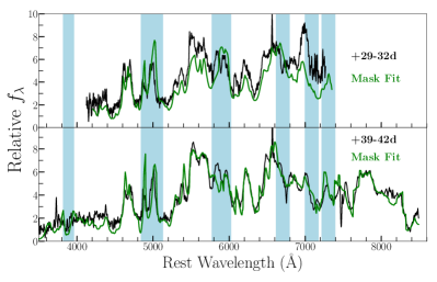
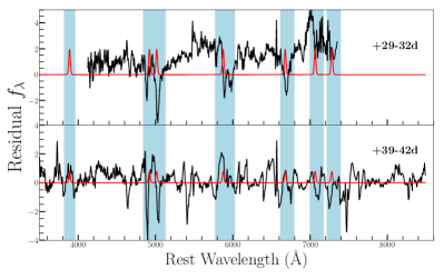
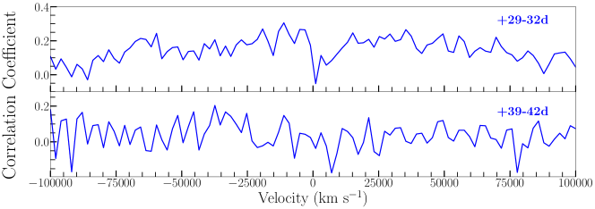
Figure 14: SN 1991bj. Phase relative to B band maximum and calculated using SNID.

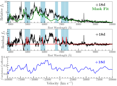
Figure 15: SN 1999ax. Phase relative to B band maximum and calculated using SNID.

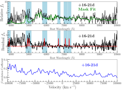
Figure 16: SN 2002bp. Phase relative to B band maximum and calculated using SNID.

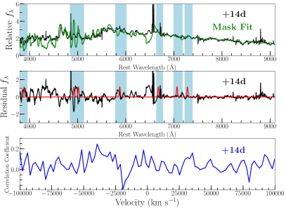
Figure 38: SN 2013dh. Phase relative to B band maximum.

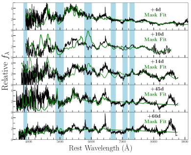
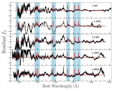
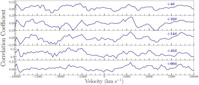
Figure 39: SN 2013en. Phase relative to B band maximum.

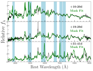
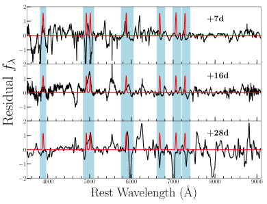
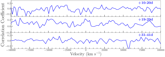
Figure 40: SN 2013gr. Phase relative to B band maximum and calculated using SNID.

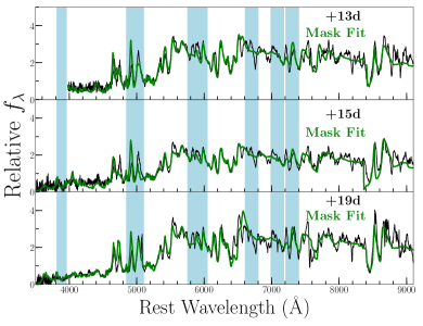
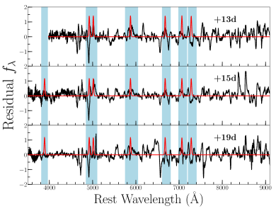
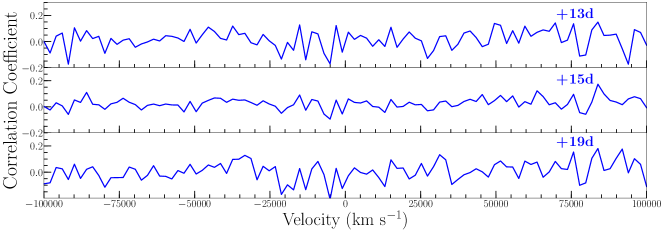
Figure 41: SN 2014ck. Phase relative to B band maximum.

Figure 42: SN 2014cr. Phase relative to B band maximum and calculated using SNID.

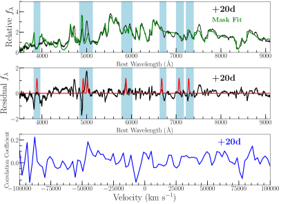
Figure 43: SN 2014dt. Phase relative to B band maximum.

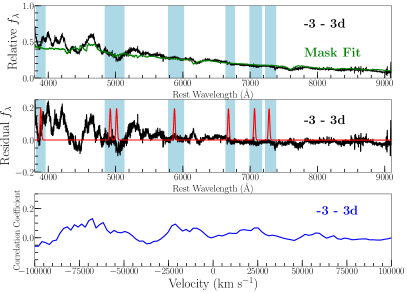
Figure 44: SN 2014ey. Phase relative to B band maximum and calculated using SNID.

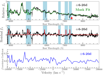
Figure 45: LSQ14dtt. Phase relative to B band maximum and calculated using SNID. Red star indicates telluric absorption.

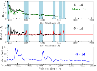
Figure 47: SN 2015ce. Phase relative to B band maximum and calculated using SNID.

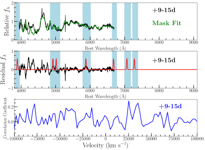
Figure 48: PS15aic. Phase relative to B band maximum and calculated using SNID.

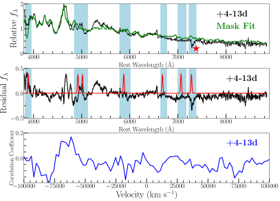
Figure 49: PS15csd. Phase relative to B band maximum and calculated using SNID. Red star indicates telluric absorption.

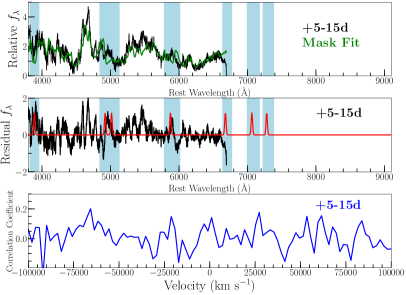
Figure 50: SN 2016atw. Phase relative to B band maximum and calculated using SNID.

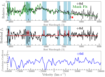
Figure 51: OGLE16erd. Phase relative to B band maximum. Red star indicates telluric absorption.

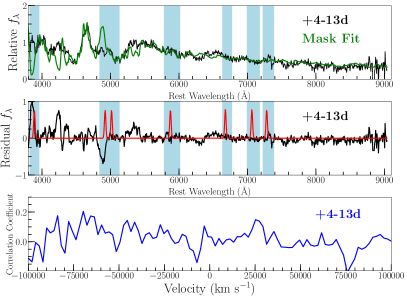
Figure 52: SN 2016ilf. Phase relative to B band maximum and calculated using SNID.

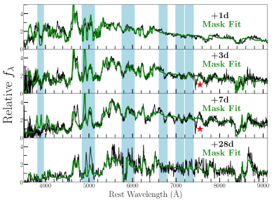
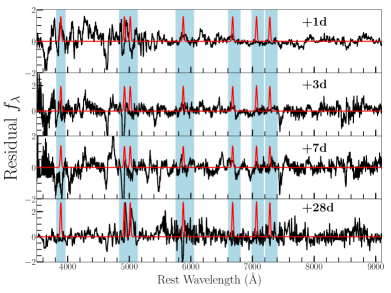
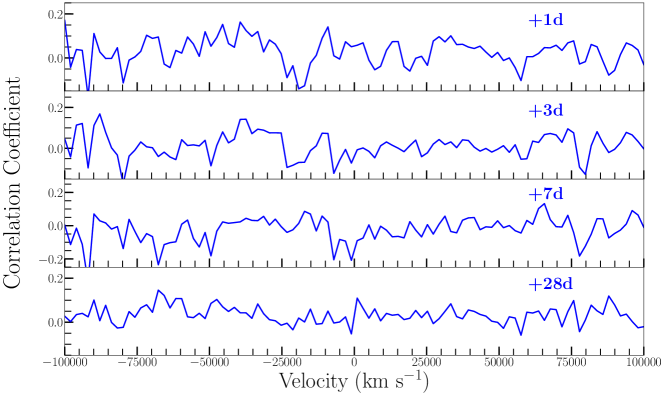
Figure 53: iPTF16fnm. Phase relative to B band maximum. Red star indicates telluric absorption.

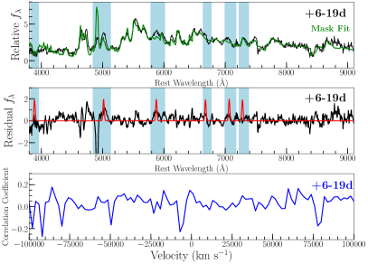
Figure 54: SN 2017gbb. Phase relative to B band maximum and calculated using SNID.

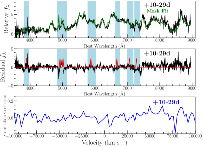
Figure 55: SN 2018atb. Phase relative to B band maximum and calculated using SNID.

References

- Balam (2017) Balam D., 2017, Transient Name Server Classification Report, 381
- Barna et al. (2018) Barna B., Szalai T., Kerzendorf W. E., Kromer M., Sim S. A., Magee M. R., Leibundgut B., 2018, MNRAS, 480, 3609
- Blondin & Tonry (2007) Blondin S., Tonry J. L., 2007, ApJ, 666, 1024
- Boehner et al. (2017) Boehner P., Plewa T., Langer N., 2017, MNRAS, 465, 2060
- Botyánszki et al. (2018) Botyánszki J., Kasen D., Plewa T., 2018, ApJ, 852, L6
- Boyle et al. (2017) Boyle A., Sim S. A., Hachinger S., Kerzendorf W., 2017, A&A, 599, A46
- Branch et al. (2004) Branch D., Baron E., Thomas R. C., Kasen D., Li W., Filippenko A. V., 2004, PASP, 116, 903
- Brooks et al. (2016) Brooks J., Bildsten L., Schwab J., Paxton B., 2016, ApJ, 821, 28
- Childress et al. (2016) Childress M. J., et al., 2016, Publ. Astron. Soc. Australia, 33, e055
- Chornock et al. (2006) Chornock R., Filippenko A. V., Branch D., Foley R. J., Jha S., Li W., 2006, PASP, 118, 722
- Copin et al. (2012) Copin Y., et al., 2012, The Astronomer’s Telegram, 4476
- Dessart & Hillier (2015) Dessart L., Hillier D. J., 2015, MNRAS, 447, 1370
- Dessart et al. (2011) Dessart L., Hillier D. J., Livne E., Yoon S.-C., Woosley S., Waldman R., Langer N., 2011, MNRAS, 414, 2985
- Dessart et al. (2012) Dessart L., Hillier D. J., Li C., Woosley S., 2012, MNRAS, 424, 2139
- Dimitriadis et al. (2016) Dimitriadis G., et al., 2016, The Astronomer’s Telegram, 9660
- Dimitriadis et al. (2018) Dimitriadis G., et al., 2018, arXiv e-prints,
- Elias-Rosa et al. (2014) Elias-Rosa N., et al., 2014, The Astronomer’s Telegram, 6398
- Filippenko et al. (2007) Filippenko A. V., Foley R. J., Silverman J. M., Chornock R., Li W., Blondin S., Matheson T., 2007, Central Bureau Electronic Telegrams, 926
- Fink et al. (2014) Fink M., et al., 2014, MNRAS, 438, 1762
- Foley et al. (2009) Foley R. J., et al., 2009, AJ, 138, 376
- Foley et al. (2013) Foley R. J., et al., 2013, ApJ, 767, 57
- Foley et al. (2015) Foley R. J., Van Dyk S. D., Jha S. W., Clubb K. I., Filippenko A. V., Mauerhan J. C., Miller A. A., Smith N., 2015, ApJ, 798, L37
- Foley et al. (2016) Foley R. J., Jha S. W., Pan Y.-C., Zheng W. K., Bildsten L., Filippenko A. V., Kasen D., 2016, MNRAS, 461, 433
- Graham et al. (2017) Graham M. L., et al., 2017, MNRAS, 472, 3437
- Graham et al. (2018) Graham M. L., et al., 2018, arXiv e-prints,
- Guillochon et al. (2017) Guillochon J., Parrent J., Kelley L. Z., Margutti R., 2017, ApJ, 835, 64
- Hachinger et al. (2012) Hachinger S., Mazzali P. A., Taubenberger S., Hillebrandt W., Nomoto K., Sauer D. N., 2012, MNRAS, 422, 70
- Hachisu et al. (1999) Hachisu I., Kato M., Nomoto K., Umeda H., 1999, ApJ, 519, 314
- Harmanen et al. (2015) Harmanen J., et al., 2015, The Astronomer’s Telegram, 8264
- Heintz et al. (2018) Heintz K. E., Malesani D., Leloudas G., D’avanzo P., Yaron O., Knezevic N., 2018, Transient Name Server Classification Report, 535
- Hillebrandt & Niemeyer (2000) Hillebrandt W., Niemeyer J. C., 2000, ARA&A, 38, 191
- Iben & Tutukov (1994) Iben Jr. I., Tutukov A. V., 1994, ApJ, 431, 264
- Jha (2017) Jha S. W., 2017, Type Iax Supernovae. p. 375, doi:10.1007/978-3-319-21846-5_42
- Jha et al. (2006) Jha S., Branch D., Chornock R., Foley R. J., Li W., Swift B. J., Casebeer D., Filippenko A. V., 2006, AJ, 132, 189
- Jordan et al. (2012) Jordan IV G. C., Perets H. B., Fisher R. T., van Rossum D. R., 2012, ApJ, 761, L23
- Kerzendorf & Sim (2014) Kerzendorf W. E., Sim S. A., 2014, MNRAS, 440, 387
- Kromer et al. (2013) Kromer M., et al., 2013, MNRAS, 429, 2287
- Leonard (2007) Leonard D. C., 2007, ApJ, 670, 1275
- Li et al. (2003) Li W., et al., 2003, PASP, 115, 453
- Liu et al. (2010) Liu W.-M., Chen W.-C., Wang B., Han Z. W., 2010, A&A, 523, A3
- Liu et al. (2012) Liu Z. W., Pakmor R., Röpke F. K., Edelmann P., Wang B., Kromer M., Hillebrandt W., Han Z. W., 2012, A&A, 548, A2
- Liu et al. (2013a) Liu Z.-W., et al., 2013a, ApJ, 774, 37
- Liu et al. (2013b) Liu Z.-W., Kromer M., Fink M., Pakmor R., Röpke F. K., Chen X. F., Wang B., Han Z. W., 2013b, ApJ, 778, 121
- Liu et al. (2015) Liu Z.-W., et al., 2015, MNRAS, 452, 838
- Lucy (1991) Lucy L. B., 1991, ApJ, 383, 308
- Lundqvist et al. (2013) Lundqvist P., et al., 2013, MNRAS, 435, 329
- Lundqvist et al. (2015) Lundqvist P., et al., 2015, A&A, 577, A39
- Lyman et al. (2013) Lyman J. D., James P. A., Perets H. B., Anderson J. P., Gal-Yam A., Mazzali P., Percival S. M., 2013, MNRAS, 434, 527
- Lyman et al. (2017) Lyman J., Homan D., Leloudas G., Yaron O., 2017, Transient Name Server Classification Report, 893
- Lyman et al. (2018) Lyman J. D., et al., 2018, MNRAS, 473, 1359
- Magee et al. (2016) Magee M. R., et al., 2016, A&A, 589, A89
- Magee et al. (2017) Magee M. R., et al., 2017, A&A, 601, A62
- Magee et al. (2019) Magee M. R., Sim S. A., Kotak R., Maguire K., Boyle A., 2019, A&A, 622, A102
- Maguire et al. (2016) Maguire K., Taubenberger S., Sullivan M., Mazzali P. A., 2016, MNRAS, 457, 3254
- Marietta et al. (2000) Marietta E., Burrows A., Fryxell B., 2000, ApJS, 128, 615
- Matheson et al. (2008) Matheson T., et al., 2008, AJ, 135, 1598
- Mattila et al. (2005) Mattila S., Lundqvist P., Sollerman J., Kozma C., Baron E., Fransson C., Leibundgut B., Nomoto K., 2005, A&A, 443, 649
- Maund et al. (2010) Maund J. R., et al., 2010, ApJ, 722, 1162
- McCully et al. (2014) McCully C., et al., 2014, Nature, 512, 54
- Miller et al. (2017) Miller A. A., et al., 2017, ApJ, 848, 59
- Nadyozhin (1994) Nadyozhin D. K., 1994, ApJS, 92, 527
- Östman et al. (2011) Östman L., et al., 2011, A&A, 526, A28
- Pan et al. (2012) Pan K.-C., Ricker P. M., Taam R. E., 2012, ApJ, 750, 151
- Pan et al. (2015) Pan Y.-C., et al., 2015, The Astronomer’s Telegram, 7519
- Pan et al. (2016) Pan Y.-C., et al., 2016, The Astronomer’s Telegram, 8810
- Parrent (2014) Parrent J. T., 2014, preprint, (arXiv:1412.7163)
- Phillips et al. (2007) Phillips M. M., et al., 2007, PASP, 119, 360
- Piersanti et al. (2014) Piersanti L., Tornambé A., Yungelson L. R., 2014, MNRAS, 445, 3239
- Postnov & Yungelson (2014) Postnov K. A., Yungelson L. R., 2014, Living Reviews in Relativity, 17, 3
- Sand et al. (2018) Sand D. J., et al., 2018, ApJ, 863, 24
- Shappee et al. (2013) Shappee B. J., Stanek K. Z., Pogge R. W., Garnavich P. M., 2013, ApJ, 762, L5
- Shappee et al. (2018) Shappee B. J., Piro A. L., Stanek K. Z., Patel S. G., Margutti R. A., Lipunov V. M., Pogge R. W., 2018, ApJ, 855, 6
- Silverman et al. (2012) Silverman J. M., et al., 2012, MNRAS, 425, 1789
- Stritzinger et al. (2014) Stritzinger M. D., et al., 2014, A&A, 561, A146
- Stritzinger et al. (2015) Stritzinger M. D., et al., 2015, A&A, 573, A2
- Szalai et al. (2015) Szalai T., et al., 2015, MNRAS, 453, 2103
- Takaro et al. (2019) Takaro T., et al., 2019, arXiv e-prints,
- Thomas et al. (2011) Thomas R. C., Nugent P. E., Meza J. C., 2011, PASP, 123, 237
- Tomasella et al. (2016) Tomasella L., et al., 2016, MNRAS, 459, 1018
- Valenti et al. (2009) Valenti S., et al., 2009, Nature, 459, 674
- Wang et al. (2013) Wang B., Justham S., Han Z., 2013, A&A, 559, A94
- Wang et al. (2015) Wang B., Li Y., Ma X., Liu D.-D., Cui X., Han Z., 2015, A&A, 584, A37
- White et al. (2015) White C. J., et al., 2015, ApJ, 799, 52
- Wood-Vasey & Sokoloski (2006) Wood-Vasey W. M., Sokoloski J. L., 2006, ApJ, 645, L53
- Woudt et al. (2009) Woudt P. A., et al., 2009, ApJ, 706, 738
- Yamanaka et al. (2015) Yamanaka M., et al., 2015, ApJ, 806, 191
- Yaron & Gal-Yam (2012) Yaron O., Gal-Yam A., 2012, PASP, 124, 668
- Yoon & Langer (2003) Yoon S.-C., Langer N., 2003, A&A, 412, L53
- Zhang et al. (2016) Zhang J., et al., 2016, The Astronomer’s Telegram, 9795