Computing closed essential surfaces in 3–manifolds

Abstract

We present a practical algorithm to test whether a 3–manifold given by a triangulation or an ideal triangulation contains a closed essential surface. This property has important theoretical and algorithmic consequences. As a testament to its practicality, we run the algorithm over a comprehensive body of closed 3–manifolds and knot exteriors, yielding results that were not previously known.

The algorithm derives from the original Jaco-Oertel framework, involves both enumeration and optimisation procedures, and combines several techniques from normal surface theory. Our methods are relevant for other difficult computational problems in 3-manifold theory, such as the recognition problem for knots, links and 3–manifolds.

57M25, 57N10

1 Introduction

In the study of 3–manifolds, essential surfaces have been of central importance since Haken’s seminal work in the 1960s. An essential surface may be regarded as ‘topologically minimal’, and there has since been extensive research into 3–manifolds, called Haken 3–manifolds, that contain an essential surface. The existence of such a surface has profound consequences for both the topology and geometry of a 3–manifold [9, 12, 18, 19, 20, 22, 23, 25, 28].

Given any closed 3–manifold, specified by a handle decomposition or triangulation, it is a theorem of Jaco and Oertel [15] from 1984 that one may algorithmically test for the existence of a closed essential surface. However, their algorithm has significant intricacies and is of doubly-exponential complexity in terms of the input size. One of the key messages of this paper is that this need not be a deterrent: with the right heuristics and careful algorithm engineering, theoretically intractable problems such as this can be implemented and automated over large sets of data.

The issue of iterated-exponential complexity, coming from cutting and re-triangulating, arises with ubiquity when considering objects called normal hierarchies. These hierarchies are key when solving more difficult problems (such as the homeomorphism problem) via Haken’s approach. Our strategy in this paper is both fast in practice and always correct and conclusive, indicating that, despite their iterated-exponential time complexities, practical implementations of these more difficult algorithms might indeed be possible.

In the remainder of this introduction, we give a summary of the theoretical results (§1.1), an overview of the algorithms (§1.2), and a summary of the computational results (§1.3).

1.1 Summary of the theoretical results

In the short conference paper [5] written with Alexander Coward, we outlined a practical implementation of the Jaco-Oertel framework for the case of finding a closed essential surface in a knot exterior in $S^{3},$ specified by an ideal triangulation. There, we introduced the bare minimum of the new theory and algorithms required for this application, not including full proofs of many of the results stated. In this paper, we generalise our results and algorithms to triangulations of closed, irreducible, orientable 3–manifolds and to ideal triangulations of the interiors of compact, irreducible and $\partial$–irreducible, orientable 3–manifolds with non-empty boundary. We thank Alexander Coward for his contributions in the early stages of this project.

We base our work on the framework of the Jaco-Oertel algorithm for testing for closed incompressible surfaces. This uses normal surfaces, which allow us to translate topological questions about surfaces into the setting of integer and linear programming. The framework consists of two stages: the first constructs a finite list of candidate essential surfaces, and the second tests each surface in the list to see if it is essential.

For the first stage (enumerating candidate essential surfaces), we combine several techniques.

First, we wish to create a triangulation for each manifold that contains as few tetrahedra as possible. This is achieved for closed 3–manifolds through the use of singular triangulations instead of simplicial ones. For compact manifolds with non-empty boundary we use ideal triangulations, which are decompositions of the interiors of these spaces into tetrahedra with their vertices removed. Ideal triangulations introduce some theoretical difficulties, but they are much smaller with roughly half as many tetrahedra.

Second, we use a variant of normal surface theory based on quadrilateral coordinates. Instead of the standard coordinates for normal surfaces involving four triangles and three quadrilaterals per tetrahedron, we work in the more efficient coordinate system only using the quadrilateral coordinates. These coordinates were known to Thurston and Jaco in the 1980s, and first appeared in print in work of Tollefson [27]. In an ideal triangulation $\mathcal{T}$ with non-spherical vertex links, this coordinate system encodes both closed normal surfaces and spun-normal surfaces, which are properly embedded and non-compact. The coordinate $x(F)$ of a closed normal surface $F$ in this spun-normal surface cone $Q(\mathcal{T})$ lies in its intersection $Q_{0}(\mathcal{T})$ with a subspace corresponding to the kernel of a boundary map (see §3.1). The following result, proven in §3.2, is based on the seminal work of Jaco and Oertel [15] and provides our finite, constructible set of candidate surfaces. An analogous result was proven by Tollefson for simplicial triangulations of closed 3–manifolds.

Theorem 5

Suppose $M$ is the interior of an irreducible and $\partial$–irreducible, compact, orientable 3–manifold with non-empty boundary, and let $\mathcal{T}$ be an ideal triangulation of $M.$ If $M$ contains a closed, essential surface $S,$ then there is a normal, closed essential surface $F$ with the property that $x(F)$ lies on an extremal ray of $Q_{0}(\mathcal{T}).$

Moreover, if $\chi(S)<0$, then there is such $F$ with $\chi(F)<0$. If, in addition, the link of each vertex has zero Euler characteristic, then if $\chi(S)=0$, then there is such $F$ with $\chi(F)=0.$

We also state Tollefon’s theorem for closed manifolds in the context of singular triangulations as Theorem 4, and give a unified proof for both theorems.

The example in §3.3 of a triangulation $\mathcal{T}_{M}$ of a trivial circle bundle over a once-punctured surface of genus two shows that our approach in Theorem 5 is optimal in the following sense. Algorithms involving normal surfaces need to reduce the search space to a finite constructible set of solutions in a cone. Typically, one chooses the set of extremal or the set of fundamental solutions. All fundamental solutions of $Q(\mathcal{T}_{M})$ are extremal, and they are either spun-normal surfaces or so-called thin-edge links, that is, closed surfaces that after one compression give a boundary parallel torus. In particular, no essential torus is amongst the fundamental solutions in $Q(\mathcal{T}_{M}).$ Hence it is necessary to consider the space $Q_{0}(\mathcal{T}_{M}).$ We thank Mark Bell for creating $\mathcal{T}_{M}$ for us with flipper [1].

1.2 Overview of the algorithms

We describe our algorithms to decide the existence of closed essential surfaces in §4. A key difficulty with the Jaco-Oertel framework, which our algorithms also inherit, is that both stages have running times that are worst-case exponential in their respective input sizes. Moreover, the output of the first stage (enumerating candidate essential surfaces) is exponential in its input, and this then becomes the input to the second stage (testing whether a candidate surface is essential). This means that combining the two stages in any obvious way leads to a doubly-exponential time complexity solution.

Despite this significant hurdle, we introduce several innovations that cut down the running time enormously for both stages. Our optimisation for the first stage involves a combination of established techniques that, though well understood individually, require new ideas and theory in order to work harmoniously together. For the second stage we combine branch-and-bound techniques from integer programming with the Jaco-Rubinstein procedure for crushing surfaces within triangulations, extending recent work of the first author and Ozlen [6].

The innovations for the second stage (testing whether a candidate surface is essential) are of particular significance, since there has never before been a systematic algorithm for testing whether a candidate surface is essential that is both practical and always conclusive. Here, the Jaco-Oertel approach cuts along each candidate surface and inspects the boundary of the resulting 3–manifold to see if it admits a compression disc (such a disc certifies that a surface is non-essential). The key difficulty is that one requires a new triangulation for the cut-open 3–manifold: since the candidate surface may be very complicated, any natural scheme for cutting and re-triangulating yields a new triangulation with exponentially many tetrahedra in the worst case, taking us far beyond the realm in which normal surface theory has traditionally been feasible in practice. Since these new triangulations are the input for stage two, which is itself exponential time, we now see where the double exponential arises, and why the Jaco-Oertel framework has long been considered far from practical.

We resolve this significant problem using a blend of techniques. First, we use strong simplification heuristics to reduce the number of tetrahedra. Next, we replace the traditional (and very expensive) enumeration-based search for compression discs with an optimisation process that maximises Euler characteristic. This uses the branch-and-bound techniques of [6], and allows us to quickly focus on a single candidate compression disc. We employ the crushing techniques of Jaco and Rubinstein [16] to quickly test whether this is indeed a compression disc, and (crucially) to reduce the size of the triangulation if it is not.

1.3 Summary of the computational results

In this paper we present a practical algorithm that, though still doubly-exponential in theory, is able to systematically test a significant class of 3–manifolds for the existence of a closed essential surface, and is both efficient in practice and always conclusive. To illustrate its power, we run this algorithm over a comprehensive body of input data, yielding computer proofs of new mathematical results.

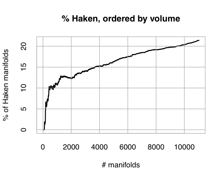
Figure 1: Haken manifolds in the Hodgson-Weeks census

We first consider the Hodgson-Weeks census, which contains 11,031 closed, orientable 3–manifolds. This is an approximation to the set of all hyperbolic 3–manifolds of volume $\leq 6.5$ and length of shortest geodesic $\geq 0.15.$ The number of tetrahedra ranges from $9$ to $32$. The first step in our algorithm is to check whether the existence of a closed essential surfaces already follows from the fact that the first Betti number is positive. Only 132 of the census manifolds ($\sim$1%) have positive Betti number, and hence are Haken for this reason. Dunfield used an implementation of the Jaco-Oertel algorithm in 1999 to compute that only 15 of the first 246 census manifolds (246/15 $\sim$ 6%) are Haken. Our computation gave the surprising result that the percentage of Haken manifolds in the Hodgson-Weeks census is about 21%, see Figure 1. Further analysis of the computation is given in §6.1.

(a) Cumulative number of knots by volume

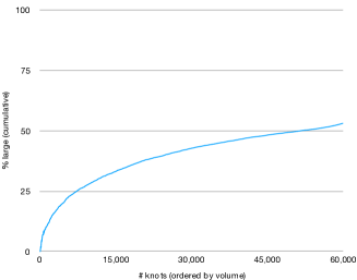
(b) Cumulative percentage of large knots

Figure 2: Percentage of large knots by volume

The next census we consider is the census of all knots in the 3–sphere with at most 14 crossings due to Hoste-Thistlethwaite-Weeks [14]. The authors thank Morwen Thistlethwaite for sharing these data with them, sorted into torus knots, satellite knots and hyperbolic knots. There are 59,924 hyperbolic knots with at most 14 crossings, and the number of ideal tetrahedra used to triangulate their complements ranges from 2 to 33. In this case, any closed essential surface is separating, and thus the algorithmic detection allows no shortcuts via homology arguments. Our computation showed that 31,805 ($\sim$ 53%) of the hyperbolic knot complements contain closed essential surfaces (we call these large knots for brevity). Figure 2 shows a cumulative plot of the percentage, where the knots in the census are ordered by volume. Further analysis of the computation is given in §6.2.

Testament to the improvement in algorithm design is the fact that Regina [4] can certify the Weber-Seifert dodecahedral space to be non-Haken out of the box in under 75 minutes on a 2016 MacBook Pro with a 3.1 GHz Intel Core i5 processor and 16 GB of 2133 MHz memory. This was a computational challenge due to Thurston when it was first solved in 2012 [8]. We caution the reader that running times are subject to random seeds and can vary significantly.

2 Preliminaries

In this section, we collect the following well-known definitions and results: singular (possibly ideal) triangulations (§2.1); essential surfaces (§2.2); a homology criterion for existence of closed essential surfaces (§2.3); normal surface theory via quadrilateral coordinates (§2.4); reduced form for Haken sums (§2.5); the Jaco-Rubinstein method of crushing of triangulations (§2.6).

2.1 Triangulations

The notation of [16] and [26] will be used in this paper. A (singular) triangulation, $\mathcal{T},$ of a compact 3–manifold $M$ consists of a union of pairwise disjoint 3–simplices, $\widetilde{\Delta}=\sigma_{1}\cup\ldots\cup\sigma_{t},$ a set of face pairings, $\Phi,$ and a homeomorphism $h\co\widetilde{\Delta}/\Phi\to M.$ We thus make the identification $\widetilde{\Delta}/\Phi=M$ and there is a natural quotient map $p\co\widetilde{\Delta}\to\widetilde{\Delta}/\Phi=M.$ The quotient map is injective on the interior of each 3–simplex. We refer to the image of a 3–simplex in $M$ as a tetrahedron and to its faces, edges and vertices with respect to the pre-image. Similarly for images of 2–, 1– and 0–simplices, which will be referred to as faces, edges and vertices in $M$ respectively. If an edge is contained in $\partial M,$ then it is termed a boundary edge; otherwise it is an interior edge.

If $M$ is the interior of a compact manifold with non-empty boundary, an ideal triangulation, $\mathcal{T},$ of $M$ consists of a union of pairwise disjoint 3–simplices, $\widetilde{\Delta},$ a set of face pairings, $\Phi,$ a natural quotient map $p\co\widetilde{\Delta}\to\widetilde{\Delta}/\Phi=P,$ and a homeomorphism $h\co P\setminus P^{(0)}\to M,$ between $M$ and the complement of the 0–skeleton in $P.$ The quotient space $P$ is usually called a pseudo-manifold and referred to as the end-compactification of $M.$

For brevity, we will refer to a 3–manifold $M$ imbued with a (possibly ideal) triangulation $\mathcal{T}=(\widetilde{\Delta},\Phi,h)$ as a triangulated 3–manifold. Throughout, we will assume that $M$ is oriented, that all tetrahedra in $M$ are oriented coherently and the tetrahedra in $\widetilde{\Delta}$ are given the induced orientation.

2.2 Surfaces in 3-manifolds

The following definition of an essential surface, along with an extensive discussion of their properties, can be found in Shalen [24], §1.5.

Definition 1 ((Essential surface)).

A properly embedded surface $S$ in the compact, irreducible, orientable 3–manifold $M$ is essential if it has the following properties:

1. $S$ is bicollared;

2. the inclusion homomorphism $\pi_{1}(S_{i})\to\pi_{1}(M)$ is injective for each component $S_{i}$ of $S$;

3. no component of $S$ is a 2–sphere;

4. no component of $S$ is boundary parallel; and

5. $S$ is non-empty.

Of interest to this paper is the following geometric interpretation of the second property, see Shalen [24] for more details. A compression disc for the surface $S$ is a disc $D\subset M$ such that $D\cap S=\partial D$ and $\partial D$ is homotopically non-trivial in $S$ (i.e. does not bound a disc on $S$). In particular, if $S$ has a compression disc, then $\pi_{1}(S_{i})\to\pi_{1}(M)$ is not injective for some component of $S.$ It follows from classical work of Papakyriakopoulos that the converse is also true. Detecting compression discs is the topic of Section 4.

2.3 Closed essential surfaces from homology

In this paper, we are interested in closed essential surfaces in a compact, irreducible, orientable 3–manifold $M$ (given by a triangulation). The universal coefficients theorem and Poincaré duality give a natural isomorphism $H_{1}(M;\mathbb{Z})\cong H_{2}(M,\partial M;\mathbb{Z}),$ and it is well-known that every non-trivial class in the latter group is represented by an essential surface in $M$. In particular, if $M$ is closed and $b_{1}(M)>0,$ then $M$ contains a (necessarily closed) essential surface. Using the intersection pairing and a standard half-lives-half-dies argument, one obtains the analogous criterion that if $\partial M\neq\emptyset$ and $2b_{1}(M)>b_{1}(\partial M),$ then $M$ contains a closed essential surface.

Since the calculation of homology with integer coefficients reduces to computing Smith Normal Form of the (generally sparse) boundary matrices, our general approach is to first check if the existence of closed essential surfaces follows from homology.

2.4 Normal surface theory

In the case, where homology does not certify the existence of a closed essential surface (or is from the outset known not to do so, as is the case for a homology 3–sphere or the complement of a knot or link in a homology 3–sphere), we use Haken’s approach to connect topology to linear programming via normal surface theory in order to search for essential surfaces. A normal surface in a (possibly ideal) triangulation $\mathcal{T}$ is a properly embedded surface which intersects each tetrahedron of $\mathcal{T}$ in a pairwise disjoint collection of triangles and quadrilaterals, as shown in Figure 3. These triangles and quadrilaterals are called normal discs. In an ideal triangulation of a non-compact 3–manifold, a normal surface may contain infinitely many triangles; such a surface is called spun-normal [26]. A normal surface may be disconnected or empty.

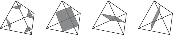
Figure 3: The seven types of normal disc in a tetrahedron.

We now describe an algebraic approach to normal surfaces. The key observation is that each normal surface contains finitely many quadrilateral discs, and is uniquely determined (up to normal isotopy) by these quadrilateral discs. Here a normal isotopy of $M$ is an isotopy that keeps all simplices of all dimensions fixed. Let $\square$ denote the set of all normal isotopy classes of normal quadrilateral discs in $\mathcal{T}$, so that $|\square|=3t$ where $t$ is the number of tetrahedra in $\mathcal{T}$. These normal isotopy classes are called quadrilateral types.

We identify $\mathbb{R}^{\square}$ with $\mathbb{R}^{3t}.$ Given a normal surface $S,$ let $x(S)\in\mathbb{R}^{\square}=\mathbb{R}^{3t}$ denote the integer vector for which each coordinate $x(S)(q)$ counts the number of quadrilateral discs in $S$ of type $q\in\square$. This normal $Q$–coordinate $x(S)$ satisfies the following two algebraic conditions.

First, $x(S)$ is admissible. A vector $x\in\mathbb{R}^{\square}$ is admissible if $x\geq 0$, and for each tetrahedron $x$ is non-zero on at most one of its three quadrilateral types. This reflects the fact that an embedded surface cannot contain two different types of quadrilateral in the same tetrahedron.

Second, $x(S)$ satisfies a linear equation for each interior edge in $M,$ termed a $Q$–matching equation. Intuitively, these equations arise from the fact that as one circumnavigates the earth, one crosses the equator from north to south as often as one crosses it from south to north. We now give the precise form of these equations. To simplify the discussion, we assume that $M$ is oriented and all tetrahedra are given the induced orientation; see [26, Section 2.9] for details.

(a) The abstract neighbourhood $B(e)$

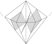
(b) Positive slope $+1$

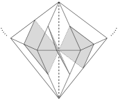
(c) Negative slope $-1$

Figure 4: Slopes of quadrilaterals

Consider the collection $\mathcal{C}$ of all (ideal) tetrahedra meeting at an edge $e$ in $M$ (including $k$ copies of tetrahedron $\sigma$ if $e$ occurs $k$ times as an edge in $\sigma$). We form the abstract neighbourhood $B(e)$ of $e$ by pairwise identifying faces of tetrahedra in $\mathcal{C}$ such that there is a well defined quotient map from $B(e)$ to the neighbourhood of $e$ in $M$; see Figure 4(a) for an illustration. Then $B(e)$ is a ball (possibly with finitely many points missing on its boundary). We think of the (ideal) endpoints of $e$ as the poles of its boundary sphere, and the remaining points as positioned on the equator.

Let $\sigma$ be a tetrahedron in $\mathcal{C}$. The boundary square of a normal quadrilateral of type $q$ in $\sigma$ meets the equator of $\partial B(e)$ if and only it has a vertex on $e$. In this case, it has a slope $\pm 1$ of a well–defined sign on $\partial B(e)$ which is independent of the orientation of $e$. Refer to Figures 4(b) and 4(c), which show quadrilaterals with positive and negative slopes respectively.

Given a quadrilateral type $q$ and an edge $e,$ there is a total weight $\operatorname{wt}_{e}(q)$ of $q$ at $e,$ which records the sum of all slopes of $q$ at $e$ (we sum because $q$ might meet $e$ more than once, if $e$ appears as multiple edges of the same tetrahedron). If $q$ has no corner on $e,$ then we set $\operatorname{wt}_{e}(q)=0.$ Given edge $e$ in $M,$ the $Q$–matching equation of $e$ is then defined by $0=\sum_{q\in\square}\;\operatorname{wt}_{e}(q)\;x(q)$.

Theorem 2.

For each $x\in\mathbb{R}^{\square}$ with the properties that $x$ has integral coordinates, $x$ is admissible and $x$ satisfies the $Q$–matching equations, there is a (possibly non-compact) normal surface $S$ such that $x=x(S).$ Moreover, $S$ is unique up to normal isotopy and adding or removing vertex linking surfaces, i.e., normal surfaces consisting entirely of normal triangles.

This is related to Hauptsatz 2 of [11]. For a proof of Theorem 2, see [21, Theorem 2.1] or [26, Theorem 2.4]. The set of all $x\in\mathbb{R}^{\square}$ with the property that (i) $x\geq 0$ and (ii) $x$ satisfies the $Q$–matching equations is denoted $Q(\mathcal{T}).$ This naturally is a polyhedral cone, but the set of all admissible $x\in\mathbb{R}^{\square}$ typically meets $Q(\mathcal{T})$ in a non-convex set.

Tollefson [27] proved the following theorem building on the work of Jaco and Oertel [15].

Theorem 3 (Tollefson).

Let $M$ be a (simplicially) triangulated, compact, irreducible, $\partial$–irreducible 3-manifold. If there exists a two-sided, incompressible, $\partial$–incompressible surface in $M$, then there exists one that is a $Q$–vertex surface.

We remark that Tollefson (and the authors he cites) work with simplicial triangulations or handlebody decompositions. A close examination of the proof in [27] reveals that it applies for (singular) triangulations, and that it also shows that if $M$ contains an essential surface, then there exists one that is a $Q$–vertex surface. We will state and prove a variant of this below (Theorem 4).

2.5 Reduced form

Let $M$ be a (ideally or materially) triangulated 3–manifold. The weight of the normal surface $F$ is the cardinality of its intersection with the 1–skeleton, $\operatorname{wt}(F)=|F\cap M^{(1)}|.$ If $F$ is closed, then its weight is finite.

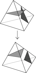
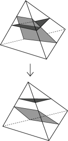
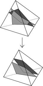
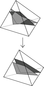
Figure 5: Regular exchange of normal discs

Two normal surfaces are compatible if they do not meet a tetrahedron in quadrilateral discs of different types. In this case, the sum of their normal coordinates is the coordinate of a normal surface. Suppose $F_{1}$ and $F_{2}$ are closed normal surfaces that are compatible, not vertex linking surfaces, and in general position. Then $x(F_{1})+x(F_{2})$ is an admissible solution to the $Q$–matching equations, and hence represented by a unique closed normal surface without vertex linking components; denote this surface $F.$ The surface $F$ is obtained geometrically as follows. At each component of $F_{1}\cap F_{2},$ there is a natural choice of regular switch between normal discs, such that the result is again a normal surface. See Figure 5 for some possible configurations involving only two discs. Denote $N(F_{1}\cap F_{2})$ a small, open, tubular neighbourhood of $F_{1}\cap F_{2}.$ The connected components of $(F_{1}\cup F_{2})\setminus N(F_{1}\cap F_{2})$ are termed patches.

Deleting any vertex linking tori that arise gives the surface $F,$ and we write $F+\Sigma=F_{1}+F_{2},$ where $\Sigma$ is a (possibly empty) finite union of vertex linking tori. This is called the Haken sum of $F_{1}$ and $F_{2}.$ Both weight and Euler characteristic are additive under this sum. So we have

$$\operatorname{wt}(F_{1})+\operatorname{wt}(F_{2}) =\operatorname{wt}(F)+\operatorname{wt}(\Sigma),$$

$$\chi(F_{1})+\chi(F_{2}) =\chi(F),$$

since $\chi(\Sigma)=0.$

The sum $F+\Sigma=F_{1}+F_{2}$ is said to be in reduced form if there is no Haken sum $F+\Sigma^{\prime}=F^{\prime}_{1}+F^{\prime}_{2},$ where $F^{\prime}_{i}$ is isotopic to $F_{i}$ in $M,$ $F^{\prime}_{1}\cap F^{\prime}_{2}$ has fewer components than $F_{1}\cap F_{2}$ and $\Sigma^{\prime}$ is a union of vertex linking tori. It should be noted that in these two sums, the embedding of $F$ in $M$ is the same (these are not equalities up to isotopy), and that any sum can be changed to a sum in reduced form.

2.6 Crushing triangulations

The crushing process of Jaco and Rubinstein [16] plays an important role in our algorithms, and we informally outline this process here. We refer the reader to [16] for the formal details, or to [3] for a simplified approach.

Let $S$ be a two-sided normal surface in a triangulation $\mathcal{T}$ of a compact orientable 3-manifold $M$ (with or without boundary). To crush $S$ in $\mathcal{T}$, we (i) cut $\mathcal{T}$ open along $S$, which splits each tetrahedron into a number of (typically non-tetrahedral) pieces, several of which are illustrated in Figure 6(a); (ii) crush each resulting copy of $S$ on the boundary to a point, which converts these pieces into tetrahedra, footballs and/or pillows as shown in Figure 6(b); and (iii) flatten each football or pillow to an edge or triangle respectively, as shown in Figure 6(c).

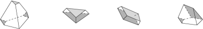
(a) Pieces after cutting open along $S$

(b) Pieces after crushing $S$ to a point

(c) Flattening footballs and pillows

Figure 6: Steps in the Jaco-Rubinstein crushing process

The result is a new collection of tetrahedra with a new set of face identifications. We emphasise that we only keep track of face identifications between tetrahedra: any “pinched” edges or vertices fall apart, and any lower-dimensional pieces (triangles, edges or vertices) that do not belong to any tetrahedra simply disappear. The resulting structure might not represent a 3-manifold triangulation, and even if it does the flattening operations might have changed the underlying 3-manifold in ways that we did not intend.

Although crushing can cause a myriad of problems in general, Jaco and Rubinstein show that in some cases the operation behaves extremely well [16]. In particular, if $S$ is a normal sphere or disc, then after crushing we always obtain a triangulation of some 3-manifold $M^{\prime}$ (possibly disconnected, and possibly empty) that is obtained from the original $M$ by zero or more of the following operations:

• cutting manifolds open along spheres and filling the resulting boundary spheres with 3-balls;

• cutting manifolds open along properly embedded discs;

• capping boundary spheres of manifolds with 3-balls;

• deleting entire connected components that are any of the 3-ball, the 3-sphere, projective space $\mathbb{R}P^{3},$ the lens space $L(3,1)$ or the product space $S^{2}\times S^{1}.$

An important observation is that the number of tetrahedra that remain after crushing is precisely the number of tetrahedra that do not contain quadrilaterals of $S$.

3 Closed normal surfaces in $Q$–space

In this section we review the linear boundary map of [26], with which we restrict the normal surface solution space to closed surfaces only, and we provide the required extensions of Jaco and Oertel’s result in the context of singular triangulations and ideal triangulations.

3.1 Boundary map

Suppose $\mathcal{T}$ is an ideal triangulation of the interior $M$ of a compact, orientable manifold with non-empty boundary. The cases we are interested in are when $M$ is irreducible and $\partial$–irreducible; or when $M$ is the complement of the set of vertices in the triangulation of a closed, irreducible 3–manifold. To keep the discussion succinct, we treat these cases together under the above more general hypothesis.

The link of an ideal vertex $v$ is an orientable surface $B_{v}$ of genus $g_{v}\geq 0$, and we may assume that $B_{v}$ is a normal surface entirely made up of normal triangles. Let $\gamma\in H_{1}(B_{v};\mathbb{R}).$ We now describe an associated linear functional $\nu(\gamma)\co\mathbb{R}^{\square}\to\mathbb{R},$ which measures the behaviour along $\gamma$ of a normal surface near the ideal vertex $v$. The idea is similar to the intuitive description of the $Q$–matching equations. As one goes along $\gamma$ and looks down into the manifold, normal quadrilaterals will (as Jeff Weeks puts it) come up from below or drop down out of sight. If the total number coming up minus the total number dropping down is non-zero, then the surface spirals towards the ideal vertex in the cross section $\gamma\times[0,\infty)\subset B_{v}\times[0,\infty)$ and the sign indicates the direction, see Figure 8(b) for a sketch when $B_{v}$ is a torus. If this number is zero, then after a suitable isotopy the surface meets the cross section in a (possibly empty) union of circles, see Figure 8(c).

The surface $B_{v}$ has an induced triangulation consisting of normal triangles. Represent $\gamma$ by an oriented path on $B_{v},$ which is disjoint from the 0–skeleton and meets the 1–skeleton transversely. Each edge of a triangle in $B_{v}$ is a normal arc. Give the edges of each triangle in $B_{v}$ transverse orientations pointing into the triangle and labelled by the quadrilateral types sharing the normal arc with the triangle; see Figure 7. We then define $\nu(\gamma)$ as follows. Choosing any starting point on $\gamma,$ we read off a formal linear combination of quadrilateral types $q$ by taking $+q$ each time the corresponding edge is crossed with the transverse orientation, and $-q$ each time it is crossed against the transverse orientation (where each edge in $B_{v}$ is counted twice—using the two adjacent triangles).

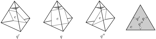
Figure 7: Coming up and dropping down

Evaluating $\nu(\gamma)$ at some $x\in\mathbb{R}^{\square}$ gives a real number $\nu_{x}(\gamma).$ For example, taking a small loop around a vertex in $T$ and setting this equal to zero gives the $Q$–matching equation of the corresponding edge in $M;$ see Figure 8(a). For each $x\in Q(\mathcal{T}),$ the resulting map $\nu_{v,x}\co H_{1}(B_{v};\mathbb{R})\to\mathbb{R}$ is a well-defined homomorphism, which has the property that the surface in Theorem 2 is closed if and only if $\nu_{v,x}=0$ (see [26], Proposition 3.3). Since $\nu_{v,x}\co H_{1}(B_{v};\mathbb{R})\to\mathbb{R}$ is a homomorphism, it is trivial if and only if we have $\nu_{v,x}(\alpha_{i})=0=\nu_{v,x}(\beta_{i})$ for any basis $\{\alpha_{i},\beta_{i}\}_{1\leq i\leq g_{v}}$ of $H_{1}(B_{v};\mathbb{R}).$

(a) $0=\nu_{x}(\gamma)=\sum_{i=1}^{k}(-1)^{i}x(q_{i})$ is the $Q$–matching equation

(b) spun $\Longleftrightarrow$ $\nu_{x}\neq 0$

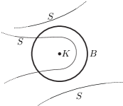
(c) not spun $\Longleftrightarrow$ $\nu_{x}=0$

Figure 8: Boundary map determines $Q$–matching equations and spinning

We define $\nu_{x}=\oplus_{v}\;\nu_{v,x},$ where the sum is taken over all ideal vertices. The surface in Theorem 2 is closed if and only if $\nu_{x}=0$ (see [26], Proposition 3.3). We then define $Q_{0}(\mathcal{T})=Q(\mathcal{T})\cap\{x\mid\nu_{x}=0\},$ and call a 2–sided, connected normal, surface $F$ with $Q(F)$ on an extremal ray of $Q_{0}(\mathcal{T})$ a $Q_{0}$–vertex surface.

We remark that if $B_{v}$ is a sphere, then $\nu_{v,x}=0$ and hence in the case where each $B_{v}$ is a sphere, we have $Q_{0}(\mathcal{T})=Q(\mathcal{T}).$

3.2 Jaco-Oertel revisited

For the algorithms of this paper, we require the following results, which are based on the seminal work of Jaco and Oertel [15].

Theorem 4.

Let $M$ be a triangulated, closed, orientable, irreducible 3-manifold. If there exists an essential surface $S$ in $M$, then there is a normal essential surface $F$ with the property that $x(F)$ lies on an extremal ray of $Q_{0}(\mathcal{T})=Q(\mathcal{T}).$

Moreover, if $\chi(S)<0$ (resp. $\chi(S)=0$), then there is such $F$ with $\chi(F)<0$ (resp. $\chi(F)=0$).

Theorem 5.

Suppose $M$ is the interior of an irreducible and $\partial$–irreducible, compact, orientable 3–manifold with non-empty boundary, and let $\mathcal{T}$ be an ideal triangulation of $M.$ If $M$ contains a closed, essential surface $S,$ then there is a normal, closed essential surface $F$ with the property that $x(F)$ lies on an extremal ray of $Q_{0}(\mathcal{T}).$

Moreover, if $\chi(S)<0$, then there is such $F$ with $\chi(F)<0$. If, in addition, the link of each vertex has zero Euler characteristic, then if $\chi(S)=0$, then there is such $F$ with $\chi(F)=0.$

Proof of Theorems 4 and 5.

Suppose $M$ contains a closed, essential surface. It follows from a standard argument (see, for instance, [15] and [16]) that there is a closed, essential, normal surface $S$ in $M.$ It remains to show that $S$ may be chosen such that $S$ is a $Q_{0}$–vertex surface. Replace $S$ by a normal surface that has least weight amongst all normal surfaces isotopic (but not necessarily normally isotopic) to $S.$ Denote this least weight surface $S$ again.

Suppose $S$ is not a $Q_{0}$–vertex surface. Then

$$nx(S)=\sum n_{i}x(V_{i}),$$

where $n,n_{i}\in\mathbb{N}$ and either $V_{i}$ or $2V_{i}$ is a $Q_{0}$–vertex surface for each $i.$ The two cases arise from the fact that we require a $Q_{0}$–vertex surface to be 2–sided and connected: If $V$ corresponds to the first integer lattice point on an admissible extremal ray of $Q_{0}(\mathcal{T})$ and $V$ is 1–sided, then the corresponding $Q_{0}$–vertex surface is $2V,$ obtained by taking the boundary of a regular neighbourhood of $V.$

We denote $nS$ the normal surface obtained by taking $n$ parallel copies of $S.$ Clearly, $x(nS)=nx(S),$ and since $S$ has least weight in its isotopy class, so does $nS$ because $S$ is 2–sided. To sum up, $nS$ is a closed, essential, normal surface which has least weight amongst all normal surfaces in its isotopy class.

For any $i,$ either $V_{i}$ or $2V_{i}$ is a $Q_{0}$–vertex surface. In the first case, we can write

$$nS+\Sigma=V+W,$$

where $\Sigma$ is a finite sum of pairwise disjoint vertex linking surfaces disjoint from $nS$, $V=V_{i}$ and $x(W)=-x(V_{i})+\sum n_{i}x(V_{i}).$ Now $nS$ is 2–sided and of least weight, so the ingenious proof of [15, Theorem 2.2] can be adapted (analogous to [21, Theorem 5.4]) to show that if one writes $nS+\Sigma=V^{\prime}+W^{\prime}$ in reduced form, then both $V^{\prime}$ and $W^{\prime}$ are two-sided and incompressible. Now $V^{\prime}$ is isotopic in $M$ to $V,$ and hence $V$ is also incompressible. If $2V_{i}$ is a $Q_{0}$–vertex surface, then we apply the above argument to $2nS,$ writing $2nS+\Sigma=V+W,$ where $x(V)=2x(V_{i})$ and $x(W)=-x(V)+2\sum n_{i}x(V_{i}).$ In either case, we obtain an incompressible $Q_{0}$–vertex surface $V.$ We will now show that $V$ is essential, i.e. that $V$ is neither a 2–sphere nor isotopic to a vertex linking surface. In doing so, we will always refer to the reduced form $mS+\Sigma=V^{\prime}+W^{\prime},$ where $m=n$ or $m=2n.$

Suppose first that $V$ is a 2–sphere. Then the 2–sphere $V^{\prime}$ bounds a ball $B$ in $M$. Now if $V^{\prime}\cap W^{\prime}$ is non-empty, then using an innermost circles argument and the fact that $W^{\prime}$ is incompressible, we obtain a contradiction to the fact that $mS+\Sigma=V^{\prime}+W^{\prime}$ is reduced. Whence $V^{\prime}\cap W^{\prime}=\emptyset.$ But since $mS+\Sigma=V^{\prime}+W^{\prime},$ this implies that either $S$ is a 2–sphere or a component of $\Sigma$ contains a quadrilateral disc, which is a contradiction. Whence $V$ is not a 2–sphere, and it follows that none of the vertex surfaces $V_{i}$ is a 2–sphere.

This, together with the fact that Euler characteristic is additive over Haken sums completes the proof of Theorem 4.

Hence assume that $M$ is non-compact and that $V$ (and therefore $V^{\prime}$) is isotopic to the link of some vertex of genus $\geq 1.$ Let $B_{v}$ be such a vertex link which is isotopic to $V^{\prime}$ and disjoint from the closed surface $W^{\prime}.$ Then there is a product region $N\cong B_{v}\times I$ in $M$ with $\partial N=B_{v}\cup V^{\prime}.$ The only incompressible and $\partial$–incompressible surfaces in $N\cong B_{v}\times I$ are isotopic to horizontal surfaces homeomorphic with $B_{v}$ or vertical annuli (and hence meet both $B_{v}$ and $V^{\prime}$).

Suppose that there is a connected component $U$ of $W^{\prime}\cap N$ with non-empty boundary. Then $\partial U\subset V^{\prime},$ and $U$ is incompressible but $\partial$–compressible in $N.$ We can therefore perform a sequence of boundary compressions, which can be promoted to an isotopy of $U$ to a subsurface of $V^{\prime}.$ Whence choosing an innermost such component $U$ of $W^{\prime}\cap N$, we see that performing regular exchanges at all intersection curves in $U\cap V^{\prime}$ gives a contradiction to the fact that $nS+\Sigma=V^{\prime}+W^{\prime}$ is reduced.

Hence $W^{\prime}\cap V^{\prime}=\emptyset.$ But then a component of $nS+\Sigma$ is isotopic but not normally isotopic to a vertex linking surface, giving the final contradiction. ∎

3.3 Example

The trivial circle bundle over a once-punctured surface of genus two has a triangulation $\mathcal{T}_{M}$ with isomorphism signature

sLLLLPLPMvQAQbefijjlklkjpqqoorrraxaaaaaaaaxhaaaahhh.

This triangulation was created for us by Mark Bell using flipper [1].

There are 29 admissible vertex solutions spanning $Q(\mathcal{T}_{M}),$ and this set is identical with the set of fundamental solutions. Exactly 9 of the corresponding fundamental surfaces are thin-edge linking surfaces of genus two. Hence after one compression they reduce to a boundary parallel torus. The remaining 20 vertex surfaces are spun-normal.

In contrast, the space $Q_{0}(\mathcal{T}_{M})$ has 81 admissible vertex solutions, and these again coincide with the admissible fundamental solutions. The corresponding surfaces are 9 thin edge linking surfaces of genus two, 4 separating essential tori and the remaining 68 are non-separating essential tori.

4 Algorithms

We present general algorithms to decide whether any 3–manifold satisfying the hypotheses of Theorems 4 or 5 contains a closed essential surface.

4.1 Non-compact manifolds

We present the algorithm in two stages below. Algorithm 6 describes a subroutine to test whether a given separating closed surface is incompressible. Algorithm 8 is the main algorithm: it uses the results of Section 3 to identify candidate essential surfaces, and runs Algorithm 6 over each.

These algorithms contain a number of high-level and often intricate procedures, many of which are described in separate papers. For each algorithm, we discuss these procedures in further detail after presenting the overall algorithm structure.

Algorithm 6 (Testing for incompressibility of separating surface).

Suppose $\mathcal{T}$ is known to be an ideal triangulation of the interior $M$ of an irreducible and $\partial$–irreducible, compact, orientable 3–manifold with non-empty boundary. Let $S$ be a separating, closed, two-sided normal surface of genus $g\geq 1$ within $\mathcal{T}$. To test whether $S$ is incompressible in $M$:

1. Truncate each ideal vertex of $\mathcal{T}$ (i.e. remove a small open neighbourhood of that vertex) to obtain a compact manifold with boundary, cut $\mathcal{T}$ open along the surface $S$, and retriangulate. The result is a pair of triangulations $\mathcal{T}_{1},\mathcal{T}_{2}$ representing two compact manifolds with boundary $M_{1},M_{2}$ (one on each side of $S$ in $M$).

   Let $S_{1},S_{2}$ be the genus $g$ boundary components of $\mathcal{T}_{1}$ and $\mathcal{T}_{2}$ respectively that correspond to the surface $S$, and let $B_{k},$ $1\leq k\leq|\partial\overline{M}|$ be the remaining boundary components of the triangulations.

2. For each $i=1,2$:

   1. Simplify $\mathcal{T}_{i}$ into a triangulation with no internal vertices and only one vertex on each boundary component, without increasing the number of tetrahedra. Let the resulting number of tetrahedra in $\mathcal{T}_{i}$ be $n$.

   2. Search for a connected normal surface $E$ in $\mathcal{T}_{i}$ that is not a vertex link, has positive Euler characteristic, and does not meet any of the boundary components $B_{k}$.

   3. If no such $E$ exists, then there is no compressing disc for $S$ in $M_{i}$. If $i=1$ then try $i=2$ instead, and if $i=2$ then terminate with the result that $S$ is incompressible.

   4. Otherwise crush the surface $E$ as explained in Section 2.6 to obtain a new triangulation $\mathcal{T}^{\prime}_{i}$ (possibly disconnected, or possibly empty) with strictly fewer than $n$ tetrahedra. If some component of $\mathcal{T}^{\prime}_{i}$ has the same genus boundary (or boundaries) as $\mathcal{T}_{i}$ then it represents the same manifold $M_{i}$, and we return to step 2a using this component of $\mathcal{T}^{\prime}_{i}$ instead. Otherwise we terminate with the result that $S$ is not incompressible.

Regarding the individual steps of this algorithm:

• Step 1 requires us to truncate an ideal vertex and cut a triangulation open along a normal surface. These are standard (though intricate) procedures. To truncate a vertex we subdivide tetrahedra and then remove the immediate neighbourhood of the vertex. To cut along a normal surface is more complex; a manageable implementation is described in [8].

• Step 2a requires us to simplify a triangulation to use the fewest possible vertices, without increasing the number of tetrahedra. For this we begin with the rich polynomial-time simplification heuristics described in [2]. In practice, for all $2979$ knots that we consider in Section 6, this is sufficient to reduce the triangulation to the desired number of vertices.

  If there are still extraneous vertices, we can remove these using the crushing techniques of Jaco and Rubinstein [16, Section 5.2]. This might fail, but only if $\partial M_{i}$ has a compressing disc, or two boundary components of $M_{i}$ are separated by a sphere; since $M$ is $\partial$–irreducible and irreducible both cases immediately certify that the surface $S$ is compressible, and we can terminate immediately.

• Step 2b requires us to locate a connected normal surface $E$ in $\mathcal{T}_{i}$ that is not a vertex link, has positive Euler characteristic, and does not any of the boundary components $B_{k}$. For this we use the recent method of [6, Algorithm 11], which draws on combinatorial optimisation techniques: in essence we run a sequence of linear programs over a combinatorial search tree, and prune this tree using tailored branch-and-bound methods. See [6] for details.

  We note that this search is the bottleneck of Algorithm 6: the search is worst-case exponential time, though in practice it often runs much faster [6]. The exposition in [6] works in the setting where the underlying triangulation is a knot complement, but the methods work equally well in our setting here. To avoid the boundary components $B_{k}$, we simply remove all normal discs that touch any of the $B_{k}$ from our coordinate system.

Theorem 7.

Algorithm 6 terminates, and its output is correct.

Proof.

The algorithm terminates because each time we loop back to step 2a we have fewer tetrahedra than before. To prove correctness, we now devote ourselves to proving the many claims that are made throughout the statement of Algorithm 6.

Before proceeding, however, we make a brief note regarding irreducibility. Since $M$ is irreducible, every embedded 2–sphere in $M$ must bound a ball. As a result, the two manifolds $M_{1}$ and $M_{2}$ are likewise irreducible, with the following possible exception. Suppose $M_{j}$ is reducible, so there is a sphere $F$ in $M_{j}$ which does not bound a ball. Since $M$ is irreducible, this sphere bounds a ball in $M$ and hence all boundary components $B_{k}$ of $M$ are on one side of this sphere. Therefore, they are all boundary components of $M_{j}$, and the sphere $F$ separates the union of all $B_{k}$ from $S_{j}.$ Whence $S$ is contained in a ball in $M$ and therefore compressible. (Note that a compression disc for $S$ may be in the reducible manifold $M_{j}$ or in the other component, which is necessarily irreducible.)

We proceed now with proofs of the various claims made in Algorithm 6.

• In step 1 we claim that cutting along $S$ yields two compact manifolds.

  This is because $S$ is a assumed to be separating.

• In step 2c we claim that, if the surface $E$ cannot be found in $\mathcal{T}_{1}$ and it cannot be found in $\mathcal{T}_{2}$, then the original surface $S$ must be incompressible.

  Suppose that $S$ were compressible, with a compression disc in some $M_{i}$. If this $M_{i}$ is irreducible, then by a result of Jaco and Oertel [15, Lemma 4.1] there is a normal compressing disc in $\mathcal{T}_{i}$. Since the underlying manifold is $\partial$–irreducible, this compressing disc must meet the genus $g$ boundary $S_{i}$ (not any of the $B_{k}$), and so it is a surface of the type we are searching for. If this $M_{i}$ is reducible then (from earlier) we have that there is a properly embedded sphere within $M_{i}$, which separates the boundary components $B_{k}$ of $M_{i}$ from $S_{i},$ so it is a surface of the type we are searching for.

• In step 2d we claim that the new triangulation $\mathcal{T}^{\prime}_{i}$ has strictly fewer tetrahedra than $\mathcal{T}_{i}$.

  This is because $E$ is connected but not a vertex link, and therefore contains at least one normal quadrilateral. As noted in Section 2.6, this means that at least one tetrahedron of $\mathcal{T}_{i}$ is deleted in the Jaco-Rubinstein crushing process.

• In step 2d we claim that if $\mathcal{T}^{\prime}_{i}$ has a component with the same genus boundary (or boundaries) as $\mathcal{T}_{i}$ then this component represents the same manifold $M_{i}$, and if not then $S$ is compressible.

  Since the surface $E$ that we crush is connected with positive Euler characteristic and can be embedded within an irreducible, orientable 3–manifold with non-empty boundary, it follows that $E$ is either a sphere or a disc. From §2.6, this means that when we crush $E$ in the triangulation $\mathcal{T}_{i}$, the resulting manifold is obtained from $M_{i}$ by a sequence of zero or more of the following operations:

  • undoing connected sums;

  • cutting open along properly embedded discs;

  • filling boundary spheres with 3–balls;

  • deleting an entire component which is homeomorphic with a 3–ball, 3–sphere, $\mathbb{R}P^{3}$, $L_{3,1}$ or $S^{2}\times S^{1}$.

  Since $M$ is irreducible and $\partial$–irreducible, cutting $M_{i}$ open along a properly embedded disc either cuts off a 3–ball or corresponds to a compression of $S_{i}.$ We now analyse the effect of crushing on $M_{i}.$

  Suppose that $M_{i}$ is irreducible. Then undoing a connected sum simply has the effect of creating an extra 3–sphere component (which will be deleted) and filling a boundary sphere with a ball. If we ever cut along a properly embedded disc that is not a compressing disc, then likewise this just creates an extra 3-ball component. If we cut along a compressing disc, then this yields one or two pieces with strictly smaller total boundary genus than before; moreover, since the underlying manifold is $\partial$–irreducible, the first such compression must take place along the genus $g$ boundary $S_{i}$ (not any $B_{k}$) and so $S$ must be compressible. Together these observations establish the full claim above: we either terminate with the correctly identified result that $S$ is compressible or return a smaller triangulation of $M_{i}$ to step 2a.

  Suppose $M_{i}$ is reducible. Then, as above, undoing a connected sum either creates extra 3–sphere components, or we have undone a non-trivial connected sum. In the latter case, one sphere in the associated collection must separate boundary components of $M_{i}$, so that no component of $\mathcal{T}^{\prime}_{i}$ has the same boundary as $\mathcal{T}_{i},$ and since this sphere certifies that $S$ is compressible the conclusion is correct. Similarly, cutting along a properly embedded disc that is not a compressing disc, creates an extra 3-ball component, whilst cutting along a compression discs changes the boundary of $M_{i}.$ Whence in this case, we also either terminate with the correctly identified result that $S$ is compressible or return a smaller triangulation of $M_{i}$ to step 2a. ∎

We can now package together a full algorithm to test for closed essential surfaces:

Algorithm 8 (Closed essential surface in ideal triangulation).

Suppose $\mathcal{T}$ is known to be an ideal triangulation of the interior $M$ of an irreducible and $\partial$–irreducible, compact, orientable 3–manifold $\overline{M}$ with non-empty boundary.

To test whether $M$ contains a closed essential surface:

1. Test whether $2b_{1}(M)>b_{1}(\partial\overline{M}).$ If yes, then terminate with the result that $M$ contains a closed essential surface.

2. Otherwise enumerate all extremal rays of $Q_{0}(\mathcal{T})$; denote these $\mathbf{e}_{1},\ldots,\mathbf{e}_{k}$. For each extremal ray $\mathbf{e}_{i}$, let $S_{i}$ be the unique connected two-sided normal surface for which $x(S_{i})$ lies on $\mathbf{e}_{i}$. From the previous step, we know that each $S_{i}$ is separating.

3. For each non-spherical surface $S_{i}$, use Algorithm 6 to test whether $S_{i}$ is incompressible in $\mathcal{T}$. If the genus of $S_{i}$ is different from the genera of the vertex links of $M$, then terminate with the result that $M$ contains a closed essential surface.

4. Now each $S_{i}$ is a sphere or has genus equal to a vertex link. So for each non-spherical surface $S_{i}$, test whether $S_{i}$ is boundary parallel by (i) cutting $\mathcal{T}$ open along $S_{i}$ and truncating all ideal vertices, and then (ii) using the Jaco-Tollefson algorithm [17, Algorithm 9.7] to test whether one of the resulting components is homeomorphic to the product space $S_{i}\times[0,1]$. If $S_{i}$ is not boundary parallel, then terminate with the result that $M$ contains a closed essential surface. Otherwise all incompressible surfaces are found to be boundary parallel, then terminate with the result that $M$ contains no closed essential surface.

Regarding the individual steps:

• Step 1 requires us to compute homology. This is a standard routine using Smith normal form, and implemented following Hafner and McCurley [10].

• Step 2 requires us to enumerate all extremal rays of $Q_{0}(\mathcal{T})$. This is an expensive procedure (which is unavoidable, since there is a worst-case exponential number of extremal rays). For this we use the recent state-of-the-art tree traversal method [7], which is tailored to the constraints and pathologies of normal surface theory and is found to be highly effective for larger problems. The tree traversal method works in the larger cone $Q(\mathcal{T})$, but it is a simple matter to insert the additional linear equations corresponding to $\nu_{x}=0$.

  We also note that it is simple to identify the unique closed two-sided normal surface for which $x(S)$ lies on the extremal ray $\mathbf{e}$. Specifically, $x(S)$ is either the smallest integer vector on $\mathbf{e}$ or, if that vector yields a one-sided surface, then its double.

• Step 4 requires us to run the Jaco-Tollefson algorithm to test whether any incompressible surface is boundary-parallel. This algorithm is expensive: it requires us to work in a larger normal coordinate system, solve difficult enumeration problems, and perform intricate geometric operations. However, in our applications, we work (mostly) with hyperbolic 3–manifolds of finite volume, for which we never enter this step. Also, in the case where the boundary of the manifold consists of tori, there are additional fast methods for avoiding the Jaco-Tollefson algorithm. For instance, one may run Haraway’s $T^{2}\times I$ test [13, Proposition 13] in conjunction with the algorithms from [6].

Theorem 9.

Algorithm 8 terminates, and its output is correct.

Proof.

The algorithm terminates because it does not contain any loops. All that remains is to prove that its output is correct.

Throughout this proof we implicitly use Theorem 7 to verify that all calls to Algorithm 6 are themselves correct. We note that the conditions of Theorem 5 apply.

From Theorem 5, the manifold $M$ contains a closed essential surface if and only if one of the closed normal surfaces $S_{i}$ in our list (excluding spheres) is essential. We ignore spheres from now onwards. We note that each surface in the list that has genus different from all vertex links is essential if and only if it is incompressible (since such a surface cannot be boundary parallel), and each remaining surface in the list is essential if and only if it is (i) incompressible and (ii) not boundary parallel.

Steps 3 and 4 of Algorithm 8 test precisely these conditions, and so the algorithm is correct. The only reason for the order in these steps is so that we can use Algorithm 6 exclusively if possible, and only fall through to the more expensive Jaco-Tollefson algorithm when absolutely necessary. ∎

4.2 Closed manifolds

For reference, we also spell out the algorithm for closed, irreducible, orientable 3–manifolds, which follows the same outline as the algorithm for non-compact 3–manifolds, but with fewer steps. Indeed, cutting along a separating normal surface in a closed 3–manifold results in two compact 3–manifolds which have a copy of this surface as a boundary component. Components of this kind are also dealt with by Algorithm 6.

Algorithm 10 (Closed essential surface in triangulation).

Suppose $\mathcal{T}$ is known to be a (possibly singular) triangulation of the closed, irreducible, orientable 3-manifold $M.$ To test whether $M$ contains a closed essential surface:

1. Test whether $b_{1}(M)>0.$ If yes, then terminate with the result that $M$ contains a closed essential surface.

2. Otherwise enumerate all extremal rays of $Q(\mathcal{T})$; denote these $\mathbf{e}_{1},\ldots,\mathbf{e}_{k}$. For each extremal ray $\mathbf{e}_{i}$, let $S_{i}$ be the unique connected two-sided normal surface for which $x(S_{i})$ lies on $\mathbf{e}_{i}$. From the previous step, we know that each $S_{i}$ is separating.

3. For each non-spherical surface $S_{i}$, cut $\mathcal{T}$ open along $S_{i}$ and retriangulate. The result is a pair of triangulations $\mathcal{T}_{1}$ and $\mathcal{T}_{2}$ representing two compact manifolds with boundary $M_{1}$ and $M_{2}.$ Let $S_{j}=\partial M_{j}.$ For each $i=1,2:$

   1. Simplify $\mathcal{T}_{i}$ into a triangulation with no internal vertices and only one vertex on its boundary component, without increasing the number of tetrahedra. Let the resulting number of tetrahedra in $\mathcal{T}_{i}$ be $n$.

   2. Search for a connected normal surface $E$ in $\mathcal{T}_{i}$ that is not a vertex link and has positive Euler characteristic.

   3. If no such $E$ exists, then there is no compressing disc for $S_{i}$ in $M_{i}$. If $i=1$ then try $i=2$ instead, and if $i=2$ then terminate with the result that $S_{i}$ is incompressible.

   4. Otherwise crush the surface $E$ as explained in Section 2.6 to obtain a new triangulation $\mathcal{T}^{\prime}_{i}$ (possibly disconnected, or possibly empty) with strictly fewer than $n$ tetrahedra. If some component of $\mathcal{T}^{\prime}_{i}$ has the same genus boundary as $\mathcal{T}_{i}$ then it represents the same manifold $M_{i}$, and we return to step 3a using this component of $\mathcal{T}^{\prime}_{i}$ instead. Otherwise we terminate with the result that $S$ is not incompressible.

   If no non-spherical surface $S_{i}$ has been found to be incompressible, terminate with the result that $M$ contains no closed essential surface.

The arguments showing that Algorithm 10 is correct and terminates are analogous to the ones given for Algorithms 6 and 8, and will therefore not be stated again.

5 Algorithm engineering and implementation

Since Algorithms 8 and 10 have doubly-exponential running times in theory, they must be implemented with great care if we are to hope for running times that are nevertheless feasible in practice.

Some of this comes down to “traditional” algorithm engineering—careful choices of data structures and code flow that make frequent operations very fast (often using trade-offs that make less frequent operations slower). Such techniques are common practice in software development, and we do not discuss them further here.

What is more important, however, is to implement the algorithms in such a way that:

• if the input to some expensive procedure is “well-structured” in a way that allows an answer to be seen quickly, then the procedure can identify this and terminate early;

• if the input is not well-structured, then the code attempts to find an equivalent input (e.g., a different triangulation of the same manifold) that does allow early termination as described above.

For Algorithms 8 and 10, the most expensive procedure is in step 3 of each algorithm, where we cut the original manifold open along a normal surface $S_{i}$ and attempt to either (i) find a compressing disc in one of the resulting triangulations $\mathcal{T}_{1}$ or $\mathcal{T}_{2}$, or (ii) certify that no such compressing disc exists.

For this procedure, the implementations in Regina are designed as follows:

• When searching for a compressing disc in each triangulation $\mathcal{T}_{j}$, we begin by optimistically checking “simple” locations in which compressing discs are often found [8].

  This includes looking for discs formed from a single face of the triangulation whose edges all lie in the boundary, or discs that slice through a single tetrahedron encircling an edge of degree one (Figure 9).

  

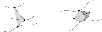
  Figure 9: Examples of simple compressing discs

  Such discs are fast to locate and check, and only if no such “simple” discs are found do we fall back to a full search (i.e., a branch-and-bound search for a normal surface with positive Euler characteristic, as described earlier in this paper).

• After cutting along $S_{i}$ to obtain the pair of triangulations $\mathcal{T}_{1}$ and $\mathcal{T}_{2}$, we search for a compressing disc in both triangulations $\mathcal{T}_{1}$ and $\mathcal{T}_{2}$ simultaneously.

  This allows the procedure to terminate early in the case where $S_{i}$ is compressible, since if we find a compressing disc in one triangulation $\mathcal{T}_{j}$ then there is no need to finish searching the other.

• Extending this idea of parallel processing further: when searching each triangulation $\mathcal{T}_{j}$ for a compressing disc, we simultaneously search through several different retriangulations of $\mathcal{T}_{j}$ (i.e., different triangulations of the same manifold with boundary).

  As before, as soon as any of these retriangulations yields a compressing disc then we can immediately terminate the entire procedure for the surface $S_{i}$ (which is now known to be compressible).

  Moreover, this parallelisation also helps in the case where $S_{i}$ is incompressible. It is often found in practice that, when searching for a compressing disc, the branch-and-bound search for a positive Euler characteristic surface finishes in remarkably few steps [6]. If this happens with any of our retriangulations then we will have certified that $\mathcal{T}_{j}$ does not contain a compressing disc, and we can immediately stop processing $\mathcal{T}_{j}$ and instead devote our attention to the manifold on the other side of $S_{i}$.

  Since the performance of the branch-and-bound code in practice depends heavily on the combinatorial structure of the underlying triangulation, it is important to choose retriangulations of $\mathcal{T}_{j}$ that are as dissimilar as possible. For this reason, the implementation in Regina creates these retriangulations immediately after cutting along $S_{i}$, before performing any simplification moves—this increases the chances that different retriangulations of $\mathcal{T}_{j}$ remain substantially different even after they are subsequently simplified. (In the worst case, if two retriangulations simplify to become combinatorially identical, then we discard the duplicate and attempt yet another retriangulation to take its place.)

• When testing the candidate incompressible surfaces $S_{i}$ in step 3 of Algorithms 8 and 10, we work through these surfaces in order from smallest genus to largest.

  This is because higher genus surfaces are likely to result in larger triangulations $\mathcal{T}_{j}$, which could potentially mean much longer running times (since testing compressibility requires exponential time in the size of $\mathcal{T}_{j}$).

  If there is no incompressible surface then the total running time is not affected (since every surface must be checked regardless). If there is an incompressible surface, however, then processing the surfaces in order by genus makes it more likely that an incompressible surface is found before the triangulations $\mathcal{T}_{j}$ become too large to handle.

We note that Algorithm 8 contains another potentialy expensive step: testing whether a surface $S_{i}$ is boundary parallel, which involves cutting along $S_{i}$ and testing whether either side forms the product $S_{i}\times[0,1]$. This procedure is not optimised in Regina, because (for this paper at least) it does not matter—in every knot complement that we processed, none of the candidate surfaces $S_{i}$ were tori (and therefore none were boundary parallel).

The discussion above only outlines the major optimisations in the implementation of Algorithms 8 and 10. For further details, the reader is encouraged to read through the thoroughly documented source code in Regina [4].

6 Computational results

This section gives some additional information about the computational results. The complete data are available at [4].

6.1 Closed manifolds

The Hodgson-Weeks census contains 11,031 closed, orientable 3–manifolds. The theoretical running time of our algorithm is $\exp(\exp(O(n))),$ where $n$ is the number of tetrahedra. As stated in the introduction, the number of tetrahedra ranges from $9$ to $32$ over the census. Figure 10 plots the running times (measuring wall time) for enumerating the candidate surfaces and deciding incompressibility.

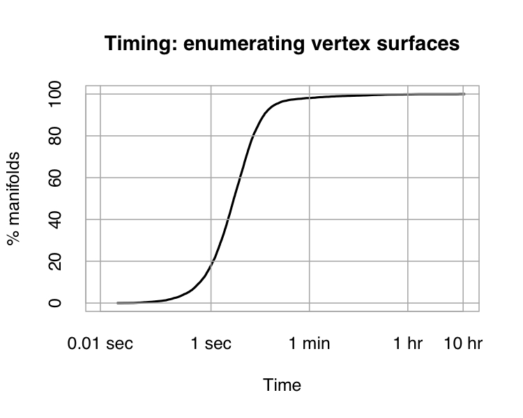
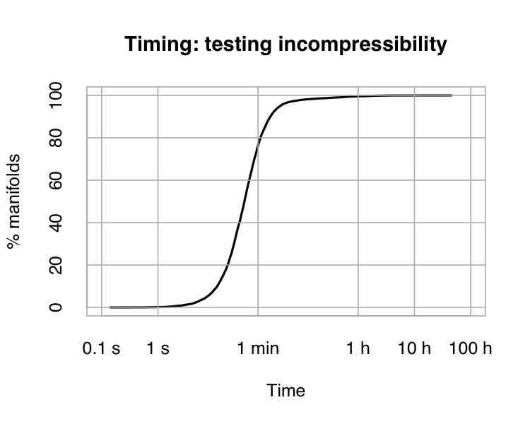
Figure 10: Timing for the Hodgson-Weeks census

Given a vertex normal surface $S$ in a triangulation of $M$ with $n$ tetrahedra we expect order of $\exp(n)$ tetrahedra in a triangulation of $M{\backslash\kern-3.20007pt\backslash}S,$ so between $10^{4}$ and $10^{14}$ tetrahedra after cutting and retriangulating for the census manifolds. Figure 11 shows that in practice the numbers are magnitutes smaller.

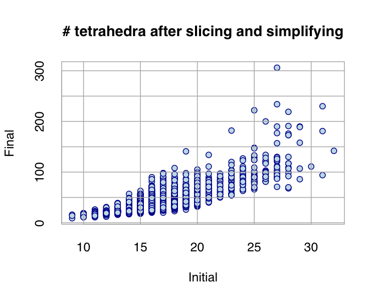
Figure 11: Number of tetrahedra after slicing and simplifying

A plot showing the percentage of Haken manifolds in the census is shown in Figure 1 in the introduction.

6.2 Knot complements

The census of all knots in the 3–sphere with at most 14 crossings due to Hoste-Thistlethwaite-Weeks [14] contains 59,924 hyperbolic knots with at most 14 crossings, and the number of ideal tetrahedra used to triangulate their complements ranges from 2 to 33. Figure 12 gives an idea of the number of tetrahedra versus the number of crossings.

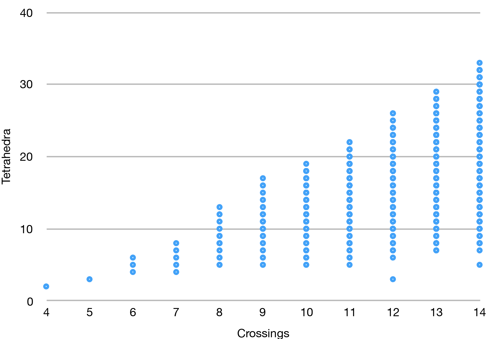
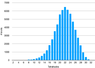
Figure 12: Numer of tetrahedra versus number of crossings

Figure 13 plots the running times (measuring wall time) for enumerating the candidate surfaces and deciding incompressibility.

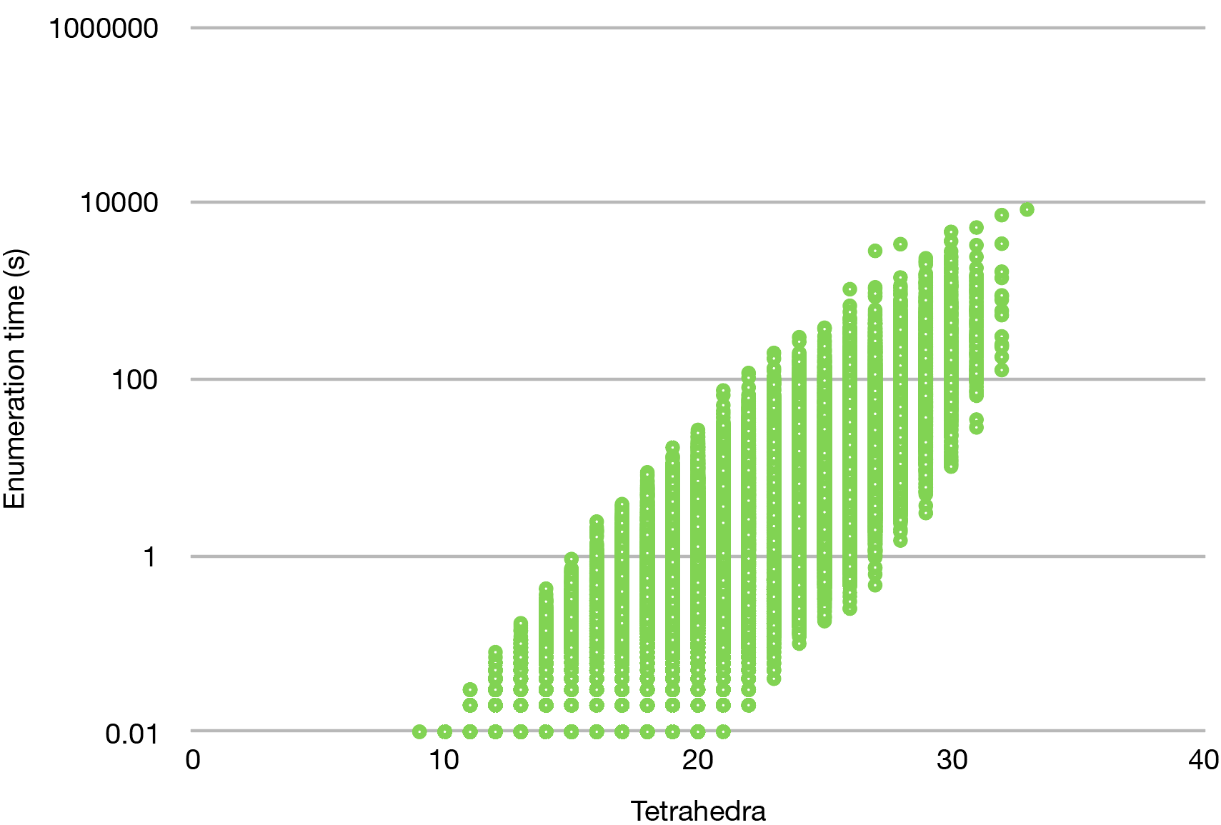
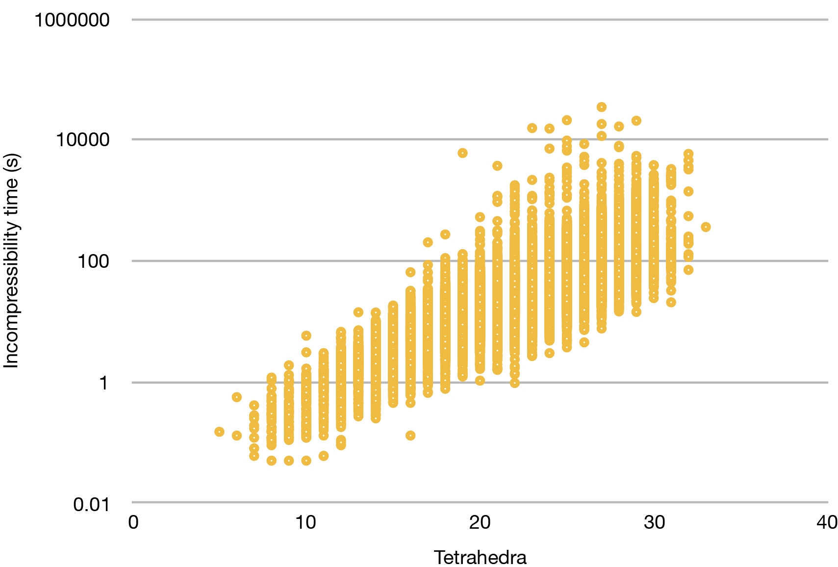
Figure 13: Timing for the Hoste-Thistlethwaite-Weeks census

We give three different perspectives of the percentage of knot diagrams containing closed essential surfaces (colloquially called large knots). Namely, by number of crossings (Figure 14), by number of tetrahedra (Figure 15) and by volume (Figure 2).

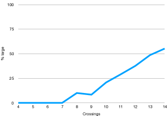
(a) Pointwise

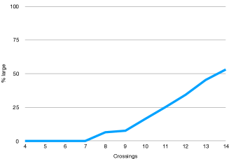
(b) Cumulative

Figure 14: Percentage of large knots by number of crossings

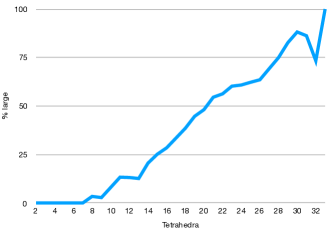
(a) Pointwise

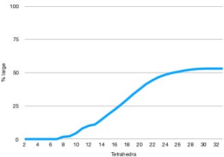
(b) Cumulative

Figure 15: Percentage of large knots by number of tetrahedra

We remark that for large numbers of tetrahedra, there are only few knot complements (see Figure 12), which explains in Figure 15 both the levelling out of the cumulative plot as well as the jumps in the pointwise plot.

Acknowledgements

The authors are supported by the Australian Research Council under the Discovery Projects funding scheme (DP150104108 and DP160104502, respectively).

References

- [1] Mark Bell, flipper (computer software), pypi.python.org/pypi/flipper, 2013–2017.
- [2] Benjamin A. Burton, Computational topology with Regina: algorithms, heuristics and implementations, Geometry and topology down under, Contemp. Math., vol. 597, Amer. Math. Soc., Providence, RI, 2013, pp. 195–224. MR 3186674
- [3] , A new approach to crushing 3-manifold triangulations, Discrete Comput. Geom. 52 (2014), no. 1, 116–139. MR 3231034
- [4] Benjamin A. Burton, Ryan Budney, William Pettersson, et al., Regina: Software for 3-manifold topology and normal surface theory, http://regina.sourceforge.net/, 1999–2012.
- [5] Benjamin A. Burton, Alexander Coward, and Stephan Tillmann, Computing closed essential surfaces in knot complements, Computational geometry (SoCG’13), ACM, New York, 2013, pp. 405–413. MR 3208239
- [6] Benjamin A. Burton and Melih Ozlen, A fast branching algorithm for unknot recognition with experimental polynomial-time behaviour, Mathematical Programming, to appear, arXiv:1211.1079, November 2012.
- [7] , A tree traversal algorithm for decision problems in knot theory and 3-manifold topology, Algorithmica 65 (2013), no. 4, 772–801.
- [8] Benjamin A. Burton, J. Hyam Rubinstein, and Stephan Tillmann, The Weber-Seifert dodecahedral space is non-Haken, Trans. Amer. Math. Soc. 364 (2012), no. 2, 911–932.
- [9] Elizabeth Finkelstein and Yoav Moriah, Tubed incompressible surfaces in knot and link complements, Topology Appl. 96 (1999), no. 2, 153–170.
- [10] James L. Hafner and Kevin S. McCurley, Asymptotically fast triangularization of matrices over rings, SIAM J. Comput. 20 (1991), no. 6, 1068–1083.
- [11] Wolfgang Haken, Theorie der Normalflächen, Acta Math. 105 (1961), 245–375.
- [12] , Some results on surfaces in 3-manifolds, Studies in Modern Topology, Studies in Mathematics, no. 5, Math. Assoc. Amer., 1968, pp. 39–98.
- [13] R. C. Haraway, III, Determining hyperbolicity of compact orientable 3-manifolds with torus boundary, ArXiv e-prints (2014).
- [14] Jim Hoste, Morwen Thistlethwaite, and Jeff Weeks, The first 1,701,936 knots, Math. Intelligencer 20 (1998), no. 4, 33–48.
- [15] William Jaco and Ulrich Oertel, An algorithm to decide if a -manifold is a Haken manifold, Topology 23 (1984), no. 2, 195–209.
- [16] William Jaco and J. Hyam Rubinstein, 0-efficient triangulations of 3-manifolds, J. Differential Geom. 65 (2003), no. 1, 61–168.
- [17] William Jaco and Jeffrey L. Tollefson, Algorithms for the complete decomposition of a closed -manifold, Illinois J. Math. 39 (1995), no. 3, 358–406.
- [18] William H. Jaco and Peter B. Shalen, Seifert fibered spaces in -manifolds, Mem. Amer. Math. Soc. 21 (1979), no. 220, viii+192.
- [19] Klaus Johannson, Homotopy equivalences of -manifolds with boundaries, Lecture Notes in Mathematics, vol. 761, Springer, Berlin, 1979.
- [20] , On the mapping class group of simple -manifolds, Topology of Low-Dimensional Manifolds (Proc. Second Sussex Conf., Chelwood Gate, 1977), Lecture Notes in Math., vol. 722, Springer, Berlin, 1979, pp. 48–66.
- [21] Ensil Kang, Normal surfaces in non-compact 3-manifolds, J. Aust. Math. Soc. 78 (2005), no. 3, 305–321.
- [22] W. Menasco, Closed incompressible surfaces in alternating knot and link complements, Topology 23 (1984), no. 1, 37–44.
- [23] Ulrich Oertel, Closed incompressible surfaces in complements of star links, Pacific J. Math. 111 (1984), no. 1, 209–230.
- [24] Peter B. Shalen, Representations of 3-manifold groups, Handbook of Geometric Topology, North-Holland, Amsterdam, 2002, pp. 955–1044.
- [25] William P. Thurston, Hyperbolic structures on -manifolds. I. Deformation of acylindrical manifolds, Ann. of Math. (2) 124 (1986), no. 2, 203–246.
- [26] Stephan Tillmann, Normal surfaces in topologically finite 3-manifolds, Enseign. Math. (2) 54 (2008), 329–380.
- [27] Jeffrey L. Tollefson, Normal surface -theory, Pacific J. Math. 183 (1998), no. 2, 359–374.
- [28] Friedhelm Waldhausen, On irreducible -manifolds which are sufficiently large, Ann. of Math. (2) 87 (1968), 56–88.