Characterization of the Most Probable Transition Paths of Stochastic Dynamical Systems with Stable Lévy Noise

Abstract

This work is devoted to the investigation of the most probable transition path for stochastic dynamical systems driven by either symmetric $\alpha$-stable Lévy motion ($0<\alpha<1$) or Brownian motion. For stochastic dynamical systems with Brownian motion, minimizing an action functional is a general method to determine the most probable transition path. We have developed a method based on path integrals to obtain the most probable transition path of stochastic dynamical systems with symmetric $\alpha$-stable Lévy motion or Brownian motion, and the most probable path can be characterized by a deterministic dynamical system.
Keywords: Symmetric $\alpha$-stable Lévy motions; Stochastic differential equations; Most probable transition path; Path integrals.

1 Introduction

Stochastic differential equations (SDEs) have been widely used to describe complex phenomena in physical, biological, and engineering systems. Transition phenomena between dynamically significant states occur in nonlinear systems under random fluctuations. Hence a practical problem is that given a stochastic dynamical system, how to capture the transition behavior between two metastable states, and then how to determine the most probable transition path. This subject has been the research topic by a number of authors [1]-[12].

In this paper, we consider the following SDE in the state space $\mathbb{R}^{k}$:

$$dX_{t}=b(X_{t})dt+dL_{t},\;\;~{}T_{0}\leq t\leq T_{f},\;\;~{}X_{T_{0}}=X_{0},$$ (1.1)

where $L_{t}$ is a $k$-dimensional symmetric $\alpha$-stable (non-Gaussian) Lévy motion in the probability space $(\Omega,\mathbb{P})$. The solution process $X_{t}$ uniquely exists under approppriate conditions on the drift term $b(x):\mathbb{R}^{k}\rightarrow\mathbb{R}^{k}$ (see the next section). Moreover, $T_{0},~{}T_{f}$ are the initial and final time instants, respectively. For simplicity, we first consider the one dimensional case ($k=1$) and will extend to higher dimensional cases ($k>1$) in Section 3.

We will also compare with the following one dimensional SDE system with (Gaussian) Browmnian motion $B_{t}$:

$$dX_{t}=b(X_{t})dt+dB_{t},\;\;~{}T_{0}\leq t\leq T_{f},\;\;~{}X_{T_{0}}=X_{0}.$$ (1.2)

The Onsager-Machlup function [1] and $Path$ $integrals$ [2, 11, 13] are two methods to study the most probable transition path of this system (1.2). The central points of these two methods were to express the transition probability (density) function of a diffusion process by means of a functional integral over paths of the process. That is for the solution process $X_{t}$, with initial time and position $(T_{0},X_{0})$ and final time and position $(T_{f},X_{f})$. In Stratonovich discretization prescription, the transition probability density $p(X_{f},T_{f}|X_{0},T_{0})$ (or denoted by $p(X_{f}|X_{0})$) is expressed as a path integral

$$p(X_{f},T_{f}|X_{0},T_{0})=\int_{\mbox{\tiny$\begin{array}[]{c}x_{T_{0}}=X_{0}\\ x_{T_{f}}=X_{f}\end{array}$}}\mathcal{D}x~{}\exp\{-\frac{1}{2}\int_{T_{0}}^{T_{f}}[(\dot{x_{s}}-b(x_{s}))^{2}+b^{\prime}(x_{s})]ds\},$$ (1.5)

where $\mathcal{L}(x,\dot{x})=\frac{1}{2}[(\dot{x}-b(x))^{2}+b^{\prime}(x)]$ is called the Lagrangian of (1.1). In Onsager-Machlup’s method, $OM(x,\dot{x})=(\dot{x}-b(x))^{2}+b^{\prime}(x)$ is called the $OM$ function. When the path $x_{t}$ is restricted in continuous functions mapping from $[T_{0},T_{f}]$ into $\mathbb{R}$, the exponent $S(x)=-\frac{1}{2}\int_{T_{0}}^{T_{f}}[(\dot{x}-b(x))^{2}+b^{\prime}(x)]ds$ is called the Onsager-Machlup action functional. Hence finding the most probable transition path is to find a path $x_{t}$ such that the Lagrangian (OM function or the action functional) to be minimum, which is called the least action principle. This leads to the Euler-Lagrangian equation by means of a variational principle when the path restricted in twice differentiable functions. For more details of $Path$ $integrals$ and applications, see [11],[14]-[17] and references therein.

In this present paper, we will determine the most probable transition path for the stochastic system with non-Gaussian noise (1.1). The situation is different from the Gaussian case (1.2). If we try to get the exponential form (containing the action functional) for the transition probability density function for the transition path as in the Gaussian case, we need to use the Fourier transformation of the probability density [18, 19] (or characteristic function). For instance, the characteristic function of a $\alpha$-stable Lévy random variable is [20, 21]

$$\psi(u)=\exp\{i\eta u-\sigma^{\alpha}|u|^{\alpha}[1-i\beta\frac{u}{|u|}w(u,\alpha)]\},$$ (1.6)

where $0<\alpha<2$ is the Lévy index, $-1\leq\beta\leq 1$ is the skewness parameter, $\eta\in\mathbb{R}$ is the shift parameter, $\sigma\in\mathbb{R}+$ the scale parameter and

$$w(u,\alpha)=\begin{cases}\tan(\frac{\pi\alpha}{2}),~{}\alpha\neq 1,\\ -\frac{2}{\pi}\ln(|u|),~{}\alpha=1.\\ \end{cases}$$ (1.7)

The density function of this random variable is

$$f(x)=\frac{1}{2\pi}\int_{-\infty}^{+\infty}\exp(-iux)\psi(u)du.$$ (1.8)

Thus it brings the Fourier integral into the density function. So for path integral representation with this density form, it is hard (and this is unlike $(\ref{pathintegral})$) to obtain a convergent action function representation of paths:

$$p(X_{f},T_{f}|X_{0},T_{0})=\lim_{n\rightarrow\infty}\int_{-\infty}^{\infty}\cdots\int_{-\infty}^{\infty}\Pi_{n}f(x_{n}-x_{n-1}-b(x_{n-1}\triangle t))\delta(x_{n}-X_{f})\mathcal{J}dx_{1}\cdots dx_{n},$$ (1.9)

where $n$ is the partition number and $\mathcal{J}$ is the Jacobian of the transformation given by

$$\begin{split}\mathcal{J}=\det(\frac{\partial L_{i}}{\partial x_{k}}),~{}i=1,\cdots,n,~{}k=1,\cdots,n.\end{split}$$ (1.10)

Instead, in this paper, we develop a method to characterize the most probable transition path, based on the path integral rather than on the action functional (or the Onsager-Machlup function). This is made possible with a new representation [22] for the transition probability density functions of symmetric Lévy motions in terms of two families of metrics. This representation provides an exponential structure of the transition probability density function [22, 23]. It can be further extended in our case, which will be discussed in Section 2.2.

This paper is organized as follows. In Section 2, we recall some preliminaries. In Section 3, we develop a method to characterize the most probable transition paths for a stochastic system with symmetric $\alpha$-stable Lévy motion ($0<\alpha<1$) or Brownian motion. In Section 4, we extend the results of Section 3 to higher dimensional cases. Finally, in Section 5, we present several examples to illustrate our results.

2 Preliminaries

2.1 Lévy motions

We recall some basic facts about 1-dimensional Lévy motions (or Lévy processes) [20, 21, 24].

Definition 1.

A stochastic process $L_{t}$ is a Lévy process if
(i) $L_{0}$=0 (a.s.);
(ii) $L_{t}$ has independent increments and stationary increments; and
(iii) $L_{t}$ has stochastically continuous sample paths, $i.e.$, for every $s\geq 0$, $L(t)\rightarrow L(s)$ in probability, as $t\rightarrow s$.

A Lévy process $L_{t}$ taking values in $\mathbb{R}$ is characterized by a drift term $\eta\in\mathbb{R}$, a non-negative variance $Q$ and a Borel measure $\nu$ defined on $\mathbb{R}\setminus\{0\}$. $(\eta,Q,\nu)$ is called the generating triplet of the Lévy motion $L_{t}$. Moreover, the Lévy-Itô decomposition for $L_{t}$ as follows:

$$L_{t}=\eta t+B_{Q}(t)+\int_{|z|<1}z\tilde{N}(t,dz)+\int_{|z|\geq 1}zN(t,dz),$$ (2.11)

where $N(dt,dz)$ is the Poisson random measure, $\tilde{N}(dt,dz)=N(dt,dz)-\nu(dz)dt$ is the compensated Poisson random measure, and $\nu(S)\triangleq\mathbb{E}N(1,S)$, here $\mathbb{E}$ denotes the expectation with respect to the probability $\mathbb{P}$, and $B_{\sigma}(t)$ is a Brownian motion with variance $\sigma$. The characteristic function of $L_{t}$ is given by

$$\mathbb{E}[\exp(iuL_{t})]=\exp(-t\psi(u)),~{}~{}u\in\mathbb{R},$$ (2.12)

where the function $\psi:\mathbb{R}\rightarrow\mathbb{C}$ is the characteristic exponent

$$\psi(u)=iu\eta+\frac{1}{2}Qu^{2}+\int_{\mathbb{R}\setminus\{0\}}(1-e^{iuz}+iuz\mathbb{I}_{\{|z|<1\}})\nu(dz).$$ (2.13)

The Borel measure $\nu$ is called the jump measure.

2.2 Asymptotic properties of the probability density functions of $\alpha$-stable Lévy motions

From now on, we consider a scalar symmetric $\alpha$-stable Lévy processes. Recall the standard symmetric $\alpha$-stable random variable has distribution $S_{\alpha}(1,0,0)$. Here $S_{\alpha}(\sigma,\beta,\mu)$ is the distribution of a stable random variable, with $\sigma$ the scale parameter, $\beta$ the skewness parameter and $\mu$ the shift parameter. The corresponding probability density function $f_{\alpha}(x)$ can be represented as an infinite series [24, 25, 26]

$$f_{\alpha}(x)=\begin{cases}\frac{1}{\pi\alpha}\sum_{k=1}^{\infty}\frac{(-1)^{k-1}}{k!}\Gamma(\alpha k+1)|x|^{-\alpha k}\sin(\frac{\alpha k\pi}{2}),&x\neq 0,~{}0<\alpha<1,\\ \frac{1}{\pi}\int_{0}^{\infty}e^{-u^{\alpha}}du,&x=0,~{}0<\alpha<1,\\ \frac{1}{\pi(1+x^{2})},&\alpha=1,\\ \frac{1}{\pi\alpha}\sum_{k=0}^{\infty}\frac{(-1)^{k}}{(2k)!}\Gamma(\frac{2k+1}{\alpha})x^{2k},&1<\alpha<2.\end{cases}$$ (2.14)

Recall the probability density function $f_{b}(x)$ for a Brownian random variable $X\sim N(0,\sigma^{2})$ is [24]

$$f_{b}(x)=\frac{1}{\sqrt{2\pi}\sigma}e^{-\frac{x^{2}}{2\sigma^{2}}}.\\$$ (2.15)

In [19], it was proved that the transition probability density function $p(x_{t}|x_{0})$ of a symmetric $\alpha$-stable Lévy process is

$$\begin{split}p(x_{t}|x_{0})&=\frac{1}{t^{1/\alpha}}f_{\alpha}(\frac{x_{t}-x_{0}}{t^{1/\alpha}})\\ &=\frac{1}{t^{1/\alpha}}\exp[-(-\ln f_{\alpha}(\frac{x_{t}-x_{0}}{t^{1/\alpha}}))]\\ &\triangleq\frac{1}{t^{1/\alpha}}\exp[-\theta^{\alpha}_{t}(x_{t}-x_{0})],\end{split}$$ (2.16)

where $\theta^{\alpha}_{t}(\cdot)$ is a function maps $[0,\infty)$ to $[0,\infty)$ for any $\alpha\in(0,2)$ and $t\in(0,\infty)$. Differentiate $\theta^{\alpha}_{t}(x)$ with respect to variable $x$:

$$\begin{split}(\theta^{\alpha}_{t}(x))^{\prime}&=(-\ln f_{\alpha}(\frac{x}{t^{1/\alpha}}))^{\prime}\\ &=-\frac{f^{\prime}_{\alpha}(\frac{x}{t^{1/\alpha}})}{f_{\alpha}(\frac{x}{t^{1/\alpha}})}\frac{1}{t^{1/\alpha}},\end{split}$$ (2.17)

which shows that $\theta^{\alpha}_{t}(\cdot)$ is a strict increase function since $f^{\prime}_{\alpha}(\frac{x}{t^{1/\alpha}})\leq 0$ for symmetric $\alpha$-stable Lévy random variables. Now we focus on the concavity of the function $\theta^{\alpha}_{t}(\cdot)$.

$$\begin{split}(\theta^{\alpha}_{t}(x))^{\prime\prime}&=(-\frac{f^{\prime}_{\alpha}(\frac{x}{t^{1/\alpha}})}{f_{\alpha}(\frac{x}{t^{1/\alpha}})}\frac{1}{t^{1/\alpha}})^{\prime}\\ &=-\frac{f_{\alpha}(\frac{x}{t^{1/\alpha}})f^{\prime\prime}_{\alpha}(\frac{x}{t^{1/\alpha}})-(f^{\prime}_{\alpha}(\frac{x}{t^{1/\alpha}}))^{2}}{f^{2}_{\alpha}(\frac{x}{t^{1/\alpha}})}\frac{1}{t^{2/\alpha}},\end{split}$$ (2.18)

In [20, 25], it was proved that if $X\sim S_{\alpha}(\sigma,\beta,\mu)$ and $\alpha\in(0,2)$,

$$\begin{split}\lim_{y\rightarrow\infty}y^{\alpha}\mathbb{P}(X>y)=C_{\alpha}\frac{1+\beta}{2}\sigma^{\alpha},\\ \lim_{y\rightarrow\infty}y^{\alpha}\mathbb{P}(X<-y)=C_{\alpha}\frac{1-\beta}{2}\sigma^{\alpha},\end{split}$$ (2.19)

where

$$C_{\alpha}=(\int_{0}^{\infty}x^{-\alpha}\sin(x)dx)^{-1}.$$ (2.20)

We use this result to study the asymptotic behavior of tail probabilities. For $y$ large enough,

$$\begin{split}&y^{\alpha}\mathbb{P}(X>y)=C_{\alpha}\frac{1+\beta}{2}\sigma^{\alpha},\\ \Leftrightarrow~{}&y^{\alpha}\int_{y}^{\infty}f_{\alpha}(x)dx=C_{\alpha}\frac{1+\beta}{2}\sigma^{\alpha},\\ \Leftrightarrow~{}&f_{\alpha}(y)=\alpha C_{\alpha}\frac{1+\beta}{2}\sigma^{\alpha}y^{-\alpha-1}\triangleq Cy^{-\alpha-1},\\ \Leftrightarrow~{}&f^{\prime\prime}_{\alpha}(y)f_{\alpha}(y)-(f^{\prime}_{\alpha}(y))^{2}=C^{2}(\alpha+1)y^{-2\alpha-4},\end{split}$$ (2.21)

which means that the asymptotic behavior of tail concavity and convexity of $\theta^{\alpha}_{t}(\cdot)$ is concave. And the graphs of $\theta^{\alpha}_{1}(\cdot)$ are shown in Figure 1.

For Brownian motion case, similar to the symmetric $\alpha$-stable Lévy motion case, the corresponding exponent is $\theta^{b}_{t}(x)=\frac{x^{2}}{2t}$, which is convex.

We also notice that

$$\begin{split}&\theta^{\alpha}_{t}(x-y)=\theta^{\alpha}_{t}(|x-y|)\triangleq\theta^{\alpha}_{t}(x,y),\\ &\theta^{b}_{t}(x-y)=\theta^{b}_{t}(|x-y|)\triangleq\theta^{b}_{t}(x,y).\end{split}$$ (2.22)

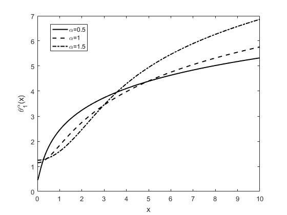
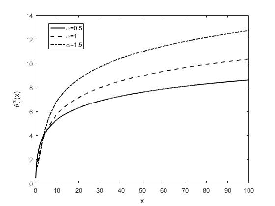
Figure 1: The graphs of function $\theta^{\alpha}_{1}(x)$ (with $\alpha=0.5,~{}1~{}$ and $1.5$): (a) on $[0,10]$; (b) on $[0,100]$.

2.3 Conditions for the well-posedness of the system (1.1) and (1.2)

For the system (1.1):

$$dX_{t}=b(X_{t})dt+dL_{t},~{}T_{0}\leq t\leq T_{f},~{}X_{T_{0}}=X_{0},$$

it was proved in [27, 28] that if $b(x)$ is locally Lipschitz continuous function and satisfies “one sided linear growth” condition in the following sense:

• C1 (Locally Lipschitz condition) For any $r>0$, there exists $K_{1}>0$ such that, for all $|y_{1}|,|y_{2}|\leq r$,

  $$|b(y_{1})-b(y_{2})|^{2}\leq K_{1}|y_{1}-y_{2}|^{2},$$

• C2 (One sided linear growth condition) There exists $K_{2}>0$ such that, for all $y\in\mathbb{R}$,

  $$2y\cdot b(y)\leq K_{2}(1+|y^{2}|),$$

then there exists a unique global solution to (1.1) and the solution is adapted and càdlàg. These two conditions also guarantee the existence and uniqueness for the solution of (1.2).

3 Method

In this section, we first study the transition behavior of the system without drift term, and then we study the general case for system (1.1) and (1.2). Before we develop the method, we present the following definition.

Definition 2.

For a solution path $X_{t}$ and the time interval $[T_{0},T_{f}]$ with a partition $T_{0}=t_{0}\leq t_{1}\leq\cdots\leq t_{n}=T_{f}$, define the sequence $\{X_{t_{0}},X_{t_{1}},\cdots,X_{t_{n}}\}$ as a discretized path of $X_{t}$. And a discretized path $\{X_{t_{0}},X_{t_{1}},\cdots,X_{t_{n}}\}$ is said to be monotonic with respect to the time partition $T_{0}=t_{0}\leq t_{1}\leq\cdots\leq t_{n}=T_{f}$ if either $X_{t_{0}}\leq X_{t_{1}}\leq\cdots\leq X_{t_{n}}$ or $X_{t_{0}}\geq X_{t_{1}}\geq\cdots\geq X_{t_{n}}$

3.1 Most probable transition path in the absence of drift

Theorem 1.

(Monotonicity for the most probable transition path in the absence of drift)
For system (1.1) and system 1.2 with drift $b\equiv 0$, every discretized path $\{X_{t_{0}},X_{t_{1}},\cdots,X_{t_{n}}\}$ of the most probable transition path is monotonic with respect to every time partition $T_{0}=t_{0}\leq t_{1}\leq\cdots\leq t_{n}=T_{f}$.

Proof.

For a time interval partition $T_{0}=t_{0}\leq t_{1}\leq t_{2}\leq\cdots\leq t_{n}=T_{f}$, define $t_{i+1}-t_{i}\triangleq\epsilon=(T_{f}-T_{0})/n,~{}i=0,1,\cdots,n-1$. (This proof is also true for an arbitrary partition.) In path integral method, the transition density function (or Markov transition probability) of $X_{t}$ of (1.1) with $b\equiv 0$ is

$$\begin{split}p(X_{f},T_{f}|X_{0},T_{0})&=\int_{-\infty}^{\infty}\cdots\int_{-\infty}^{\infty}dx_{t_{1}}\cdots dx_{{t_{n-1}}}p_{\epsilon}(x_{t_{1}}|X_{0})p_{\epsilon}(x_{t_{2}}|x_{t_{1}})\cdots p_{\epsilon}(X_{f}|x_{{t_{n-1}}})\\ &=\int\mathcal{D}_{n}x~{}\exp\{-\theta^{\alpha}_{\epsilon}(x_{{t_{1}}},X_{0})-\sum_{i=1}^{n-2}\theta^{\alpha}_{\epsilon}(x_{{t_{i+1}}},x_{t_{i}})-\theta^{\alpha}_{\epsilon}(X_{f},x_{{t_{n-1}}})\}\\ &\triangleq\int\mathcal{D}_{n}x~{}\exp\{-\sum_{i=0}^{n-1}\theta^{\alpha}_{\epsilon}(x_{{t_{i+1}}},x_{t_{i}})\}\\ &\triangleq\int\mathcal{D}_{n}x~{}\exp\{-\mathcal{S}_{n}(x)\},\end{split}$$ (3.23)

where $\mathcal{D}_{n}x=\epsilon^{-1/\alpha}\prod_{i=1}^{n-1}\epsilon^{-1/\alpha}dx_{t_{i}}$. Note that $x$ of $\mathcal{S}_{n}(x)$ is a path connecting $(T_{0},X_{0})$ and $(T_{f},X_{f})$ ($i.e.$ it starts at $X_{0}$ at the time $t=T_{0}$ and reaches $X_{f}$ at the time $t=T_{f}$). We call $\mathcal{S}_{n}(x)$ the action quantity of $x$. The contribution of a path $x_{t}$ to the transition probability density $p_{t}(X_{f},T_{f}|X_{0},T_{0})$ depends on $\mathcal{S}_{n}(x)=\sum_{i=0}^{n-1}\theta^{\alpha}_{\epsilon}(x_{{t_{i+1}}},x_{t_{i}})$.

In order to find the most probable transition path $u_{t}$, we are supposed to find it satisfies that

$$\mathcal{S}_{n}(u_{t})=\min_{x_{t}\in D_{X_{0}}^{X_{f}}}\mathcal{S}_{n}(x_{t}),$$ (3.24)

where $D_{X_{0}}^{X_{f}}$ denotes the set of paths that connect $(T_{0},X_{0})$ and $(T_{f},X_{f})$. Equivalently

$$\frac{\mathcal{S}_{n}(x_{t})}{\mathcal{S}_{n}(u_{t})}\geq 1,$$ (3.25)

for every path $x_{t}$ connecting $(T_{0},X_{0})$ and $(T_{f},X_{f})$. Here $n$ goes to infinity, and the $\lim_{n\rightarrow\infty}$ is dropped for now for clarity.

Without loss of generality, we set $X_{0}<X_{f}$. When $n=2$ (the time partition is $\{T_{0}=t_{0}<t_{1}<t_{2}=T_{f}\}$), for a path $x_{t}$ connecting $(T_{0},X_{0})$ and $(T_{f},X_{f})$, $\mathcal{S}_{2}(x_{t})=\theta^{\alpha}_{\epsilon}(x_{t_{1}},X_{0})+\theta^{\alpha}_{\epsilon}(X_{f},x_{t_{1}})$, if $x_{t_{1}}<X_{0}$. Since $\theta^{\alpha}_{\epsilon}(\cdot)$ is a strictly increasing function, together with $|x_{t_{1}}-X_{0}|>|X_{0}-X_{0}|=0$ and $|X_{f}-x_{t_{1}}|>|X_{f}-X_{0}|$, we have $\mathcal{S}_{2}(x_{t})>\theta^{\alpha}_{\epsilon}(X_{0},X_{0})+\theta^{\alpha}_{\epsilon}(X_{0},X_{f})$ where $\{X_{0},x_{t_{1}}=X_{f},X_{f}\}$ is a discretized path of a certain transition path connecting $(T_{0},X_{0})$ and $(T_{f},X_{f})$. The case that $x_{t_{1}}>X_{f}$ is similar. When we add time partitions the situation is similar again. Thus the discretized path $\{X_{t_{0}},X_{t_{1}},\cdots,X_{t_{n}}\}$ of the most probable transition path of $X_{t}$ is supposed to be monotonic with respect to the time partition, otherwise there exists a path whose action quantity is smaller.

For system (1.2), the proof is similar. ∎

The reason that we use (3.25) to find the most probable transition path is: For symmetric $\alpha$-stable Lévy motion case, the corresponding action quantity $\mathcal{S}_{n}(x_{t})$ goes to infinity as long as $n$ goes to infinity for any path $x_{t}\in D_{X_{0}}^{X_{f}}$ (since $\mathcal{S}_{n}(x_{t})\geq n\theta_{\epsilon}^{\alpha}(0)$ and $\theta_{\epsilon}^{\alpha}(0)$ is a positive constant. Here $n\theta_{\epsilon}^{\alpha}(0)$ is the action quantity of the path $X_{t}\equiv X_{0}$, $t\in[T_{0},T_{f}]$). For simplicity we say the action quantity of $x_{t}$ has higher order than $u_{t}$ if

$$\lim_{n\rightarrow\infty}\frac{\mathcal{S}_{n}(x_{t})-n\theta_{\epsilon}^{\alpha}(0)}{\mathcal{S}_{n}(u_{t})-n\theta_{\epsilon}^{\alpha}(0)}=+\infty.$$ (3.26)

That is, we compare the action quantities of two paths with the help of the fixed path ($X_{t}\equiv X_{0}$, $t\in[T_{0},T_{f}]$), which considers $X_{t}\equiv X_{0}$ $(t\in[T_{0},T_{f}])$ as a reference path. It helps us to compare the action quantities easily, which will be shown in the proof of Corollary 1. Actually,

$$\mathcal{S}_{n}(u_{t})-n\theta_{\epsilon}^{\alpha}(0)$$

$$= \sum_{i=1}^{n}\theta_{\epsilon}^{\alpha}(x_{i},x_{i-1})-n\theta_{\epsilon}^{\alpha}(0)$$

$$= \sum_{i=1}^{n}[\theta_{\epsilon}^{\alpha}(x_{i},x_{i-1})-\theta_{\epsilon}^{\alpha}(0)]$$

$$= \sum_{i=1}^{n}[-\ln f_{\alpha}(x_{i}-x_{i-1})+\ln f_{\alpha}(0)]$$

$$= \sum_{i=1}^{n}[-\ln\frac{f_{\alpha}(x_{i}-x_{i-1})}{f_{\alpha}(0)}].$$

Denoting $g_{\alpha}(x_{i}-x_{i-1})=\frac{f_{\alpha}(x_{i}-x_{i-1})}{f_{\alpha}(0)}$, the function $g_{\alpha}(\cdot)$ could be regarded as a new “probability” density function whose integration over $(-\infty,\infty)$ is $\frac{1}{f_{\alpha}(0)}$.

The most probable transition path might not be unique, $i.e.$, there might be several paths satisfying (3.24) or (3.25). In fact we will see in the following corollary that, for system (1.1), the number of the most probable transition paths is infinity but they can be characterized by a class of paths that have only one jump, and the difference among the paths of this class is the jump time. See Remark 1 after the proof of the following corollary.

Corollary 1.

(i) For system (1.1) with $b\equiv 0$, if $L_{t}$ is a symmetric $\alpha$-stable Lévy noise with $0<\alpha<1$, then the most probable transition path is not unique, and it can be represented as a $Heaviside$-like function

$$X^{m}_{t}=\begin{cases}X_{0},~{}~{}T_{0}\leq t<t^{*},\\ X_{f},~{}~{}t^{*}\leq t\leq T_{f},\\ \end{cases}$$ (3.27)

for every time instant $t^{*}$ satisfying $T_{0}<t^{*}\leq T_{f}$;

(ii) For system (1.2) with drift $b\equiv 0$, the most probable transition path is the line segment connecting $X_{0}$ and $X_{f}$: $X^{m}_{t}=X_{0}+\frac{t-T_{0}}{T_{f}-T_{0}}(X_{f}-X_{0})$;

Proof.

(i) For system (1.1) with drift $b\equiv 0$, as shown in Section 2, we notice that for a time interval partition $T_{0}=t_{0}\leq t_{1}\leq\cdots\leq t_{n}=T_{f}$, $t_{i+1}-t_{i}=\epsilon=\frac{T_{f}-T_{0}}{n}$,

$$\theta^{\alpha}_{\epsilon}(|x-y|)=\theta^{\alpha}_{1}(|\frac{x-y}{\epsilon^{1/\alpha}}|)=\theta^{\alpha}_{1}(n^{\alpha}|\frac{x-y}{(T_{f}-T_{0})^{1/\alpha}}|).$$ (3.28)

Define a path space $DM_{X_{0}}^{X_{f}}=\{x_{t}|~{}x_{t}$ is a monotonic path connects $(T_{0},X_{0})$ and $(T_{f},X_{f})$}. So one should search for the most probable transition path within path space $DM_{X_{0}}^{X_{f}}$.

Take a path $x_{t}\in DM_{X_{0}}^{X_{f}}$ and a time partition $\{T_{0}=t_{0}<t_{1}<\cdots<t_{n}=T_{f}\}$. Assume that $\{\lambda_{j}\}_{j=0}^{n-1}$ are non-negative constants, and $x_{t_{j+1}}-x_{t_{j}}=\lambda_{j}(X_{f}-X_{0})$ $(0\leq j\leq n-1)$. It is easy to see that $\sum_{j=0}^{n-1}\lambda_{j}=1$ by the Theorem 1, and $0\leq\lambda_{j}\leq 1$. As discussed in Section 2.2, $\theta^{\alpha}_{1}(\cdot)$ is concave in $[r,\infty)$ for some constant $r\in\mathbb{R}^{+}$ ($r$ depending on $\alpha$).

For $n^{1/\alpha}\lambda_{j}|\frac{X_{f}-X_{0}}{(T_{f}-T_{0})^{1/\alpha}}|\triangleq n^{1/\alpha}\lambda_{j}C_{0f}\geq r$, and $n$ large enough, we obtain

$$\begin{split}\theta^{\alpha}_{\epsilon}(|x_{t_{j+1}}-x_{t_{j}}|)-c&=\theta^{\alpha}_{1}(n^{1/\alpha}\lambda_{j}|\frac{X_{f}-X_{0}}{(T_{f}-T_{0})^{1/\alpha}}|)-c\\ &\geq\lambda_{j}(\theta^{\alpha}_{1}(n^{1/\alpha}|\frac{X_{f}-X_{0}}{(T_{f}-T_{0})^{1/\alpha}}|)-c)\\ &=\lambda_{j}(\theta^{\alpha}_{\epsilon}(|X_{f}-X_{0}|)-c),\end{split}$$ (3.29)

where $c=\theta^{\alpha}_{\epsilon}(0)$ is a positive constant and $\theta^{\alpha}_{1}(\cdot)-c$ is non-negative and concave in $[r,\infty)$.

When $n^{1/\alpha}\lambda_{j}C_{0f}<r$, we have

$$\begin{split}0\leq\sum_{n^{1/\alpha}\lambda_{j}C_{0f}<r}\lambda_{j}<n\frac{r}{n^{1/\alpha}C_{0f}},\end{split}$$ (3.30)

and

$$\begin{split}\lim_{n\rightarrow\infty}\sum_{n^{1/\alpha}\lambda_{j}C_{0f}<r}\lambda_{j}=0,~{}\lim_{n\rightarrow\infty}\sum_{n^{1/\alpha}\lambda_{j}C_{0f}\geq r}\lambda_{j}=1.\end{split}$$ (3.31)

Hence

$$\begin{split}&\lim_{n\rightarrow\infty}\mathcal{(}{S}_{n}(x_{t})-n\theta_{\epsilon}^{\alpha}(0))/\{[(n-1)\theta_{\epsilon}^{\alpha}(0)+\theta^{\alpha}_{1}(n^{1/\alpha}C_{0f})]-n\theta_{\alpha}^{\epsilon}(0)\}\\ &=\lim_{n\rightarrow\infty}[\sum_{j=0}^{n-1}\theta^{\alpha}_{1}(n^{1/\alpha}\lambda_{j}C_{0f})-n\theta_{\epsilon}^{\alpha}(0)]/[\theta^{\alpha}_{1}(n^{1/\alpha}C_{0f})-\theta_{\epsilon}^{\alpha}(0)]\\ &=\lim_{n\rightarrow\infty}[\sum_{n^{1/\alpha}\lambda_{j}C_{0f}<r}(\theta^{\alpha}_{1}(n^{1/\alpha}\lambda_{j}C_{0f})-\theta_{\epsilon}^{\alpha}(0))+\sum_{n^{1/\alpha}\lambda_{j}C_{0f}\geq r}(\theta^{\alpha}_{1}(n^{1/\alpha}\lambda_{j}C_{0f})-\theta_{\epsilon}^{\alpha}(0))]/(\theta^{\alpha}_{1}(n^{1/\alpha}C_{0f})-\theta_{\epsilon}^{\alpha}(0))\\ &\geq\lim_{n\rightarrow\infty}\sum_{n^{1/\alpha}\lambda_{j}C_{0f}\geq r}(\theta^{\alpha}_{1}(n^{1/\alpha}\lambda_{j}C_{0f})-\theta_{\epsilon}^{\alpha}(0))/(\theta^{\alpha}_{1}(n^{1/\alpha}C_{0f})-\theta_{\epsilon}^{\alpha}(0))\\ &\geq\lim_{n\rightarrow\infty}\sum_{n^{1/\alpha}\lambda_{j}C_{0f}\geq r}\lambda_{j}(\theta^{\alpha}_{1}(n^{1/\alpha}C_{0f})-\theta_{\epsilon}^{\alpha}(0))/(\theta^{\alpha}_{1}(n^{1/\alpha}C_{0f})-\theta_{\epsilon}^{\alpha}(0))\\ &=\lim_{n\rightarrow\infty}\sum_{n^{1/\alpha}\lambda_{j}C_{0f}\geq r}\lambda_{j}\\ &=1.\end{split}$$ (3.32)

This means that the most probable transition path for symmetric $\alpha$-stable Lévy process ($0<\alpha<1$) is a $Heaviside$-like function

$$X^{m}_{t}\triangleq\begin{cases}X_{f},~{}~{}t\geq t^{*},\\ X_{0},~{}~{}t<t^{*},\\ \end{cases}$$ (3.33)

or

$$X^{m}_{t}\triangleq\begin{cases}X_{f},~{}~{}t>t^{*},\\ X_{0},~{}~{}t\leq t^{*},\\ \end{cases}$$ (3.34)

where $t^{*}$ satisfies $T_{0}\leq t^{*}\leq T_{f}$. Hence in this case, the most probable transition path is not unique since the “jump time” $t^{*}$ can be chosen arbitrarily.

(ii) For system (1.2) with $b\equiv 0$, by Theorem 1 and the fact that $\theta^{b}_{\epsilon}(\cdot)$ being convex, we conclude that

$$\begin{split}\sum_{i=0}^{n-1}\theta^{b}_{\epsilon}(x_{t_{i+1}},x_{t_{i}})&=\sum_{i=0}^{n-1}\theta^{b}_{\epsilon}(|x_{{t_{i+1}}}-x_{t_{i}}|)\\ &\geq n\theta^{b}_{\epsilon}(\sum_{i=0}^{n-1}\frac{1}{n}|x_{{t_{i+1}}}-x_{t_{i}}|)\\ &=n\theta^{b}_{\epsilon}(\frac{1}{n}|X_{f}-X_{0}|).\end{split}$$ (3.35)

The inequality holds if and only if

$$\begin{split}\theta^{b}_{\epsilon}(x_{t_{1}},x_{t_{0}})=\theta^{b}_{\epsilon}(x_{t_{2}},x_{t_{1}})=\cdots=\theta^{b}_{\epsilon}(x_{{t_{n}}},x_{{t_{n-1}}})\\ \Leftrightarrow x_{t_{1}}-x_{t_{0}}=x_{t_{2}}-x_{t_{1}}=\cdots=x_{{t_{n}}}-x_{{t_{n-1}}}.\end{split}$$ (3.36)

So the most probable transition path is the line segment which connects the initial and final points. Therefore, we obtain

$$X^{m}_{t_{i}}=\frac{i(X_{f}-X_{0})}{n},~{}i=1,2,\cdots,n-1.$$ (3.37)

When $n$ goes to infinity, $X^{m}_{t}=X_{0}+\frac{t-T_{0}}{T_{f}-T_{0}}(X_{f}-X_{0})$. This implies that the most probable transition path is the path for the particle (i.e., solution) moving in constant velocity. ∎

Remark 1.

For symmetric $\alpha$-stable Lévy motion with $0<\alpha<1$, the proof of Corollary 1 compares the transition paths’ action quantities in path-wise sense. We now study the probability over all paths starting at $X_{0}$ at time $T_{0}$ and conditioned at a given end point $X_{f}$ at time $T_{f}$, to find the particle at point $X$ at time $t\in[T_{0},T_{f}]$. This probability can be written as (without loss of generality we assume $X_{f}>X_{0}$)

$$\begin{split}\mathcal{P}(X,t)&=\frac{p(X,t|X_{0},T_{0})p(X_{f},T_{f}|X,t)}{p(X_{f},T_{f}|X_{0},T_{0})}\\ &=\frac{1}{p(X_{f},T_{f}|X_{0},T_{0})}\frac{1}{|t-T_{0}|^{1/\alpha}|T_{f}-t|^{1/\alpha}}f_{\alpha}(\frac{X-X_{0}}{|t-T_{0}|^{1/\alpha}})f_{\alpha}(\frac{X_{f}-X}{|T_{f}-t|^{1/\alpha}}),\end{split}$$ (3.38)

which was studied by [30, 31]. So when $t$ is fixed, the probability $\mathcal{P}(X,t)$ is a function depending on $f_{\alpha}(\frac{X-X_{0}}{|t-T_{0}|^{1/\alpha}})f_{\alpha}(\frac{X_{f}-X}{|T_{f}-t|^{1/\alpha}})$. Note that $f_{\alpha}(\frac{X-X_{0}}{|t-T_{0}|^{1/\alpha}})$ has a peak at $X_{0}$, and $f_{\alpha}(\frac{X_{f}-X}{|T_{f}-t|^{1/\alpha}})$ has a peak at $X_{f}$. Thus the product $f_{\alpha}(\frac{X-X_{0}}{|t-T_{0}|^{1/\alpha}})f_{\alpha}(\frac{X_{f}-X}{|T_{f}-t|^{1/\alpha}})$ increases as $X\uparrow X_{0}$ and decreases as $X\downarrow X_{f}$. That is, the product reaches the global maximal value in $[X_{0},X_{f}]$. Suppose that $X_{0}\leq X\leq X_{f}$. The product can be rewritten as

$$\begin{split}f_{\alpha}(\frac{X-X_{0}}{|t-T_{0}|^{1/\alpha}})f_{\alpha}(\frac{X_{f}-X}{|T_{f}-t|^{1/\alpha}})=\exp(-(\theta^{\alpha}_{t-T_{0}}(X-X_{0})+\theta^{\alpha}_{T_{f}-t}(X_{f}-X))).\end{split}$$ (3.39)

Hence

$$\begin{split}&\theta^{\alpha}_{t-T_{0}}(X-X_{0})+\theta^{\alpha}_{T_{f}-t}(X_{f}-X)\\ =&\theta^{\alpha}_{1}(\frac{X_{f}-X_{0}}{|t-T_{0}|^{1/\alpha}}\frac{X-X_{0}}{X_{f}-X_{0}})+\theta^{\alpha}_{1}(\frac{X_{f}-X_{0}}{|T_{f}-t|^{1/\alpha}}\frac{X_{f}-X}{X_{f}-X_{0}})\\ \geq&\frac{X-X_{0}}{X_{f}-X_{0}}\theta^{\alpha}_{1}(\frac{X_{f}-X_{0}}{|t-T_{0}|^{1/\alpha}})+\frac{X_{f}-X}{X_{f}-X_{0}}\theta^{\alpha}_{1}(0)+\frac{X_{f}-X}{X_{f}-X_{0}}\theta^{\alpha}_{1}(\frac{X_{f}-X_{0}}{|T_{f}-t|^{1/\alpha}})+\frac{X-X_{0}}{X_{f}-X_{0}}\theta^{\alpha}_{1}(0)\\ \geq&(\frac{X-X_{0}}{X_{f}-X_{0}}+\frac{X_{f}-X}{X_{f}-X_{0}})\min\{\theta^{\alpha}_{1}(\frac{X_{f}-X_{0}}{|t-T_{0}|^{1/\alpha}}),\theta^{\alpha}_{1}(\frac{X_{f}-X_{0}}{|T_{f}-t|^{1/\alpha}})\}+\theta^{\alpha}_{1}(0)\\ =&\min\{\theta^{\alpha}_{1}(\frac{X_{f}-X_{0}}{|t-T_{0}|^{1/\alpha}}),\theta^{\alpha}_{1}(\frac{X_{f}-X_{0}}{|T_{f}-t|^{1/\alpha}})\}+\theta^{\alpha}_{1}(0),\end{split}$$ (3.40)

where the first inequality approximately holds if the function $\theta_{1}^{\alpha}(\cdot)$ is approximately considered as a concave function in $[0,\infty]$ (or when $\frac{X_{f}-X_{0}}{|t-T_{0}|^{1/\alpha}}$ and $\frac{X_{f}-X_{0}}{|T_{f}-t|^{1/\alpha}}$ are large enough).

Thus $\mathcal{P}(X,t)$ reaches the maximal value at $X_{0}$ when $t\in[T_{0},\frac{T_{f}+T_{0}}{2}]$, and it reaches the maximal value at $X_{f}$ when $t\in[\frac{T_{f}+T_{0}}{2},T_{f}]$. At time $\frac{T_{f}+T_{0}}{2}$, the maximal value of $\mathcal{P}(X,t)$ is reached at $X_{0}$ and $X_{f}$, simultaneously. It thus appears that the transition process jumps at the time instant $\frac{T_{f}+T_{0}}{2}$ most probably.

Inspired by this related observation, we could choose $t^{*}=\frac{T_{f}+T_{0}}{2}$ in Corollary 1, considering the transition process in time-point-wise sense. This is one plausible option that leads to the specific most probable path.

Corollary 2.

For symmetric $\alpha$-stable Lévy motions with $0<\alpha<1$, in $n$-partition path integral representation $(\ref{pdf})$ (that is, the time interval $[T_{0},T_{f}]$ has partition: $T_{0}=t_{0}\leq t_{1}\leq t_{2}\leq\cdots\leq t_{n}=T_{f}$), if the action quantity $\mathcal{S}_{n}(x_{t})$ of a path $x_{t}$ has more than one non-zero term, then we have

$$\begin{split}\lim_{n\rightarrow\infty}\frac{S_{n}(x_{t})-n\theta_{\epsilon}^{\alpha}(0)}{S_{n}(u_{t})-n\theta_{\epsilon}^{\alpha}(0)}=+\infty.\end{split}$$ (3.41)

Here $u_{t}\in D_{X_{0}}^{X_{f}}$ satisfies

$$\begin{split}du_{t}=0,~{}t\in[T_{0},T_{f}]\setminus\{t^{*}\},\end{split}$$ (3.42)

where $t^{*}\in[T_{0},T_{f}]$.

Proof.

Suppose that $C_{1},C_{2},C_{3}$ are positive constants. We obtain

$$\begin{split}&[\theta^{\alpha}_{\epsilon}(C_{1})+\theta^{\alpha}_{\epsilon}(C_{2})-2\theta^{\alpha}_{\epsilon}(0)]/(\theta^{\alpha}_{\epsilon}(C_{3})-\theta^{\alpha}_{\epsilon}(0))\\ =&[-\ln f_{\alpha}(\frac{C_{1}}{\epsilon^{1/\alpha}})-\ln f_{\alpha}(\frac{C_{2}}{\epsilon^{1/\alpha}})+2\ln f_{\alpha}(0)]/[-\ln f_{\alpha}(\frac{C_{3}}{\epsilon^{1/\alpha}})+\ln f_{\alpha}(0)]\\ =&\ln\{f^{2}_{\alpha}(0)/[f_{\alpha}(\frac{C_{1}}{\epsilon^{1/\alpha}})f_{\alpha}(\frac{C_{2}}{\epsilon^{1/\alpha}})]-f_{\alpha}(0)/(f_{\alpha}(\frac{C_{3}}{\epsilon^{1/\alpha}}))\}\\ \sim&\ln[C^{-2}f^{2}_{\alpha}(0)(\frac{C_{1}}{\epsilon^{1/\alpha}})^{1+\alpha}(\frac{C_{2}}{\epsilon^{1/\alpha}})^{1+\alpha}-C^{-1}f_{\alpha}(0)(\frac{C_{3}}{\epsilon^{1/\alpha}})^{1+\alpha}]\\ =&\ln[C^{-2}f^{2}_{\alpha}(0)(\frac{C_{1}C_{2}}{\epsilon^{2/\alpha}})^{1+\alpha}-C^{-1}f_{\alpha}(0)(\frac{C_{3}}{\epsilon^{1/\alpha}})^{1+\alpha}]\rightarrow+\infty~{}(\epsilon\rightarrow 0).\end{split}$$ (3.43)

The $\sim$ part and the positive constant $C$ come from the asymptotic behavior of $f_{\alpha}(\cdot)$ in (2.21). The formula (3.43) means that when the jump number of a path is greater, the action quantity of that path has higher order. In $n$-partition path integral representation, if the action quantity $S_{n}(x_{t})=\sum_{i=0}^{n-1}\theta^{\alpha}_{\epsilon}(x_{{t_{i+1}}},x_{t_{i}})$ of a path $x_{t}$ has more than one non-zero term, without loss of generality, we assume $\theta^{\alpha}_{\epsilon}(x_{{t_{1}}},x_{t_{0}})\neq 0$ and $\theta^{\alpha}_{\epsilon}(x_{{t_{2}}},x_{t_{1}})\neq 0$. Construct a path $\tilde{x}_{t}$:

$$\tilde{x}_{t}=\begin{cases}X_{0},~{}~{}T_{0}\leq t<t_{1},\\ x_{t_{1}},~{}~{}t_{1}\leq t<t_{2},\\ x_{t_{2}},~{}~{}t_{2}\leq t<T_{f},\\ X_{f},~{}~{}t=T_{f}.\end{cases}$$ (3.44)

Applying Corollary $(\ref{lemmaconvex})$ for these two paths in three intervals: $T_{0}\leq t<t_{1}$, $t_{1}\leq t<t_{2}$, and $t_{2}\leq t\leq T_{f}$, we have

$$\lim_{n\rightarrow\infty}\frac{S_{n}(x_{t})-n\theta_{\epsilon}^{\alpha}(0)}{S_{n}(\tilde{x}_{t})-n\theta_{\epsilon}^{\alpha}(0)}\geq 1.$$

According to (3.43),

$$\begin{split}\lim_{n\rightarrow\infty}\frac{S_{n}(\tilde{x}_{t})-n\theta_{\epsilon}^{\alpha}(0)}{S_{n}(u_{t})-n\theta_{\epsilon}^{\alpha}(0)}=+\infty,\end{split}$$ (3.45)

where $u_{t}$ satisfies $du_{t}=0,~{}t\in[T_{0},T_{f}]\setminus\{t^{*}\}$ for any $t^{*}\in[T_{0},T_{f}]$. ∎

3.2 Most probable transition path in the case of non-zero drift

Theorem 2.

(Characterization of the most probable transition path with drift term)
For system (1.1) and system (1.2), assume that the transition probability density exists, and that the most probable transition path $X^{m}_{t}$ exists and satisfies the integrability condition $|\int_{T_{0}}^{t}b(X^{m}_{s})ds|<\infty$ for $t\in[T_{0},T_{f}]$.

(i) For system (1.1) with $L_{t}$ a symmetric $\alpha$-stable Lévy motion with $(0<\alpha<1)$, the most probable transition path $X^{m}_{t}$ is determined by the following deterministic dynamical system (i.e., an ordinary differential equation),

$$\begin{cases}dX^{m}_{t}-b(X^{m}_{t})dt=0,~{}t\in[T_{0},T_{f}]\backslash\{t^{*}\},\\ X^{m}_{T_{0}}=X_{0},~{}X^{m}_{T_{f}}=X_{f},\\ \end{cases}$$ (3.46)

(ii) For system (1.2) with Brownian motion, the most probable transition path $X^{m}_{t}$ is determined by the following deterministic dynamical system (i.e., an integral-differential equation),

$$\begin{split}X^{m}_{t}-X_{0}-\int_{T_{0}}^{t}b(X^{m}_{s})ds=\frac{t-T_{0}}{T_{f}-T_{0}}(X_{f}-X_{0}-\int_{T_{0}}^{T_{f}}b(X^{m}_{s})ds),\end{split}$$ (3.47)

if $|X_{f}-X_{0}-\int_{T_{0}}^{T_{f}}b(X^{m}_{s})ds|\leq\inf_{U_{t}\in D_{X_{0}}^{X_{f}}}|X_{f}-X_{0}-\int_{T_{0}}^{T_{f}}b(U_{s})ds|$.

Proof.

For the system (1.1), the corresponding stochastic integral equation is

$$\begin{split}&X_{t}=\int_{T_{0}}^{t}b(X_{s})ds+L_{t},\\ &Y_{t}\triangleq X_{t}-\int_{T_{0}}^{t}b(X_{s})ds=L_{t},\end{split}$$ (3.48)

and the differential form is

$$\begin{split}X_{t_{i+1}}-X_{t_{i}}-[\gamma b(X_{t_{i+1}})+(1-\gamma)b(X_{t_{i}})]\triangle t=L_{t_{i+1}}-L_{t_{i}}.\\ \end{split}$$ (3.49)

In Itô interpretation ($\gamma=0$),

$$\begin{split}X_{t_{i+1}}-X_{t_{i}}-b(X_{t_{i}})\triangle t=L_{t_{i+1}}-L_{t_{i}}.\\ \end{split}$$ (3.50)

The transition probability density function of $X_{t}$ is

$$\begin{split}&p(X_{f},T_{f}|X_{0},T_{0})\\ =&\int_{-\infty}^{\infty}\cdots\int_{-\infty}^{\infty}dL_{1}\cdots dL_{n-1}dL_{n}p_{\epsilon}(L_{1}|L_{T_{0}})p_{\epsilon}(L_{2}|L_{1})\cdots p_{\epsilon}(L_{n}|L_{n-1})\delta(x_{t_{n}}-X_{f})\\ =&\int\mathcal{D}_{n+1}x\mathcal{J}\exp\{-\sum_{i=0}^{n}\theta^{\alpha}_{\epsilon}(x_{{t_{i+1}}}-x_{t_{i}}-b(x_{t_{i}})\triangle t)\}\delta(x_{t_{n}}-X_{f})\\ =&\int\mathcal{D}_{n+1}x\exp\{-\sum_{i=0}^{n}\theta^{\alpha}_{\epsilon}(x_{{t_{i+1}}}-x_{t_{i}}-b(x_{t_{i}})\triangle t)\}\delta(x_{t_{n}}-X_{f})\\ =&\int\mathcal{D}_{n+1}y\exp\{-\sum_{i=0}^{n}\theta^{\alpha}_{\epsilon}(y_{{t_{i+1}}},y_{t_{i}})\}\delta(x_{t_{n}}-X_{f}),\end{split}$$ (3.51)

where $\mathcal{J}$ is the Jacobian of the transformation given by

$$\begin{split}\mathcal{J}=\det(\frac{\partial L_{i}}{\partial x_{k}})=\prod_{i=1}^{n}(1-\epsilon\gamma\frac{db(x_{i})}{dx_{i}}).\end{split}$$ (3.52)

Assume that the most probable transition path of $X_{t}$ exist, which is denoted by $X^{m}_{t}$.

(i) For system (1.1), in order to determine the most probable transition path $X^{m}_{t}$, we consider the transition of the process $Y_{t}$ from $Y_{T_{0}}=X_{0}$ to $Y_{T_{f}}=X_{f}-\int_{T_{0}}^{T_{f}}b(X^{m}_{s})ds$. We should notice that the transition process of $Y_{t}$ is different from the one of $X_{t}$. Given the quantities $\{X_{0},X_{f},T_{0},T_{f}\}$. The diffusion process $X_{t}$ transfers from initial point $X_{0}$ at time $T_{0}$ to terminal point $X_{f}$ at time $T_{f}$. That is, all transition paths have the same initial and terminal points. But for process $Y_{t}$, the transition paths set of $Y_{t}$ is

$$D_{Y}=\{y_{t}:y_{t}=x_{t}-\int_{T_{0}}^{t}b(x_{s})ds,~{}x_{t}\in D_{X_{0}}^{X_{f}}\}.$$ (3.53)

Thus the paths in $D_{Y}$ have the same initial point $X_{0}$ but their terminal points may be different.

Since $L_{t}$ is an $\alpha$-stable Lévy motion with $0<\alpha<1$, by Corollary 2, the most probable transition path of $Y_{t}$ (denoted by $Y^{m}_{t}$) among $D_{Y}$ is presumably to satisfy

$$\begin{split}dY^{m}_{t}=0,~{}t\in[T_{0},T_{f}]\setminus\{t^{*}\},\end{split}$$ (3.54)

where $t^{*}\in[T_{0},T_{f}]$.

That is

$$\left\{\begin{array}[]{l}dX^{m}_{t}-b(X^{m}_{t})dt=0,\\ X^{m}_{T_{0}}=X_{0},~{}X^{m}_{T_{f}}=X_{f},~{}t\in[T_{0},T_{f}]\backslash\{t^{*}\}.\\ \end{array}\right.$$ (3.55)

It means that the most probable transition path has one jump and the jump size is $J_{t^{*}}=|X_{0}-\int_{T_{0}}^{t^{*}}b(X^{m}_{s})ds-X_{f}+\int_{T_{f}}^{t^{*}}b(X^{m}_{s})ds|$. In the proof of Corollary 2, if $C_{1}>C_{3}>0$ and $C_{2}=0$, the limit is still the infinity. This means the order of action quantity depends on the jump size.

So the jump time $t^{*}$ is supposed to be the one which satisfies

$$\begin{split}J_{t^{*}}=\min_{T_{0}\leq t\leq T_{f}}J_{t}.\end{split}$$ (3.56)

As $J_{t}$ is continuous in $t$, the minimizer $t^{*}$ exists (although it may not be unique).

In other words, the most probable transition path consists of two components: One component is part of the solution of equation

$$\left\{\begin{array}[]{l}dX(t)-b(X(t))dt=0,~{}t\in[T_{0},T_{f}],\\ X(T_{0})=X_{0},\\ \end{array}\right.$$ (3.57)

and the other component is part of the solution of equation

$$\left\{\begin{array}[]{l}dX(t)-b(X(t))dt=0,~{}t\in[T_{0},T_{f}],\\ X(T_{f})=X_{f}.\\ \end{array}\right.$$ (3.58)

The jump time $t^{*}$ is the moment at which $J_{t^{*}}$ is minimum.

(ii) For system (1.2), if the initial and terminal points are deterministic, then by Corollary 1, the most probable transition path of a Brownian motion is the one which connects the initial and terminal points directly. Actually the action quantity of this most probable transition path can be computed exactly provided the equal time partition in (3.35). That is,

$$\begin{split}&n\theta^{b}_{\epsilon}(\frac{1}{n}|X_{f}-X_{0}|)\\ =&n\frac{(|X_{f}-X_{0}|/n)^{2}}{2\epsilon}\\ =&n\frac{(|X_{f}-X_{0}|/n)^{2}}{2\frac{T_{f}-T_{0}}{n}}\\ =&\frac{1}{2}\frac{(X_{f}-X_{0})^{2}}{T_{f}-T_{0}}.\end{split}$$ (3.59)

Notice that $|Y_{T_{f}}-Y_{T_{0}}|=|X_{f}-X_{0}-\int_{T_{0}}^{T_{f}}b(X_{s})ds|$ is the distance between the initial and terminal points of $Y_{t}$. Then the most probable transition path of $Y_{t}$ (denoted by $Y^{m}_{t}$) can be obtained exactly,

$$\begin{split}Y^{m}_{t}&=X^{m}_{t}-X_{0}-\int_{T_{0}}^{t}b(X^{m}_{s})ds\\ &=Y_{0}+(Y_{f}-Y_{0})\frac{t-T_{0}}{T_{f}-T_{0}}\\ &=\frac{t-T_{0}}{T_{f}-T_{0}}(X_{f}-X_{0}-\int_{T_{0}}^{T_{f}}b(X^{m}_{s})ds).\end{split}$$ (3.60)

This means if there is a transition path $X^{m}_{t}\in D_{X_{0}}^{X_{f}}$ such that the formula $(\ref{bre})$ holds, then the path $X^{m}_{t}$ is the most probable one among the paths whose terminal point is $X_{f}-\int_{T_{0}}^{T_{f}}b(X^{m}_{s})ds$. So if $|X_{f}-X_{0}-\int_{T_{0}}^{T_{f}}b(X^{m}_{s})ds|\leq\inf_{U_{t}\in D_{X_{0}}^{X_{f}}}|X_{f}-X_{0}-\int_{T_{0}}^{T_{f}}b(U_{s})ds|$, then $X^{m}_{t}$ will be the most probable transition path of $X_{t}$.

This completes the proof of this theorem. ∎

Remark 2.

For a symmetric $\alpha$-stable Lévy motion with $1\leq\alpha<2$, the equalities $(\ref{control})$ do not hold. Define the path space $\mbox{DMS}_{X_{0}}^{X_{f}}\triangleq\{x_{t}|~{}x_{t}=\sum_{i=0}^{n-1}a_{i}\mathbb{I}_{[t_{i},t_{i+1})}+a_{n}\mathbb{I}_{\{T_{f}\}},T_{0}=t_{0}\leq t_{1}\leq\cdots\leq t_{n}=T_{f},X_{0}=a_{0}\leq a_{1}\leq\cdots\leq a_{n}=X_{f}\}$, where $\mathbb{I}_{B}$ is the characteristic function of set $B\subset\mathbb{R}$.

If we search for the most probable transition path within the simple path space $DMS_{X_{0}}^{X_{f}}$ for the symmetric $\alpha$-stable Lévy motion with $1\leq\alpha<2$, the similar results of Lemma 1 and Theorem 2 hold. This is because for every fixed simple path in $DMS_{X_{0}}^{X_{f}}$, the non-zero $\lambda_{j}$ of $\{\lambda_{j}\}_{j=0}^{n-1}$ are bounded below. Thus the inequality (3.29) holds for every non-negative $\lambda_{j}$, for $n$ large enough.

Remark 3.

For simplicity, we call the solution of (3.57) the initial transition path, and call the solution of (3.58) the final transition path. Consequently, the most probable transition path starts from the initial transition path and jumps to the final transition path at the time that initial transition path and final transition path are closed to each other.

Remark 4.

For the case with a symmetric $\alpha$-stable Lévy motion ($0<\alpha<1$), we are interested in the transitions between metastable states of the stochastic dynamical system $(\ref{firstequation})$. That is, the initial and terminal points $X_{0}$ and $X_{f}$ are stable points of the corresponding undisturbed system of 1.1. In this case, the initial transition path is $X_{t}=X_{0},~{}t\in[T_{0},T_{f}]$ and the final transition path is $X_{t}=X_{f},~{}t\in[T_{0},T_{f}]$ by Theorem 2 (i).

Thus the process $Y_{t}=X_{t}+\int_{T_{0}}^{T_{f}}b(X_{s})ds$ is a symmetric $\alpha$-stable Lévy motion which transits from $X_{0}$ to $X_{f}$ most probably. The most probable transition path of $Y_{t}$ provided the initial and terminal points $X_{0}$ and $X_{f}$ (as discussed in Remark 1) is

$$\begin{cases}Y^{m}_{t}=X_{0},~{}t\in[T_{0},\frac{T_{f}+T_{0}}{2}),\\ Y^{m}_{t}=X_{f},~{}t\in[\frac{T_{f}+T_{0}}{2},T_{f}].\\ \end{cases}$$ (3.61)

Thus in Theorem 2 (i), if the initial and terminal points $X_{0}$ and $X_{f}$ are metastable points of the system, the time $\frac{T_{f}+T_{0}}{2}$ can also be considered as the most probable jump time $t^{*}$.

Remark 5.

For the case with Brownian motion, the condition $|X_{f}-X_{0}-\int_{T_{0}}^{T_{f}}b(X^{m}_{s})ds|\leq\inf_{U_{t}\in D_{X_{0}}^{X_{f}}}|X_{f}-X_{0}-\int_{T_{0}}^{T_{f}}b(U_{s})ds|$ is not easy to verify. The action functional in Itô sense is $\mathcal{L}(x,\dot{x})=\frac{1}{2}(\dot{x}-b(x))^{2}$. If we assume the most probable path and the function $b(x)$ are smooth enough, then the Euler-Lagrange equation is

$$\begin{split}&~{}~{}\frac{\partial}{\partial t}\frac{\partial\mathcal{L}}{\partial\dot{x}}=\frac{\partial\mathcal{L}}{\partial x}\\ \Rightarrow&~{}~{}\ddot{x}-b^{\prime}(x)\dot{x}=-(\dot{x}-b(x))b^{\prime}(x)\\ \Rightarrow&~{}~{}\ddot{x}-b^{\prime}(x)b(x)=0.\\ \end{split}$$ (3.62)

And in our method,

$$\begin{split}&~{}~{}X^{m}_{t}-X_{0}-\int_{T_{0}}^{t}b(X^{m}_{s})ds=\frac{t-T_{0}}{T_{f}-T_{0}}(X_{f}-X_{0}-\int_{T_{0}}^{T_{f}}b(X^{m}_{s})ds)\\ \Rightarrow&~{}~{}\dot{X}^{m}_{t}-b(X^{m}_{t})=\frac{1}{T_{f}-T_{0}}(X_{f}-X_{0}-\int_{T_{0}}^{T_{f}}b(X^{m}_{s})ds)\\ \Rightarrow&~{}~{}\ddot{X}^{m}_{t}-b^{\prime}(X^{m}_{t})\dot{X}^{m}_{t}=0.\\ \end{split}$$ (3.63)

So in general, the path of (3.47) does not coincide with direct minimizer of the Onsager-Machlup’s functional. Our method is restricted here because the condition $|X_{f}-X_{0}-\int_{T_{0}}^{T_{f}}b(X^{m}_{s})ds|\leq\inf_{U_{t}\in D_{X_{0}}^{X_{f}}}|X_{f}-X_{0}-\int_{T_{0}}^{T_{f}}b(U_{s})ds|$ is not satisfied. But if the drift term $b(x)$ is independent of $x$, the integration $\int_{T_{0}}^{T_{f}}b(U_{s})ds$ is a constant for any path $U_{t}\in D_{X_{0}}^{X_{f}}$, and the two methods provide the same most probable path.

3.3 Existence, uniqueness and numerical simulation for the most probable transition path.

3.3.1 Non-Gaussian noise: System with a symmetric $\alpha$-stable Lévy motion with $0<\alpha<1$.

The most probable transition path is determined by two “initial” value problems of a deterministic ordinary differential equation (ODE)

$$\begin{cases}dX^{m}_{t}-b(X^{m}_{t})dt=0,~{}t\in[T_{0},T_{f}]\backslash\{t^{*}\},\\ X^{m}_{T_{0}}=X_{0},~{}X^{m}_{T_{f}}=X_{f},~{}t^{*}\in[T_{0},T_{f}].\\ \end{cases}$$ (3.64)

The first initial value problem solves this ODE with $X^{m}_{T_{0}}=X_{0}$, and the second problem solves this ODE backward in time with terminal value condition $X^{m}_{T_{f}}=X_{f}$. The existence and uniqueness of these solutions are ensured by the local Lipschitz continuity of the drift term $b(x)$.

Given a time partition $\{T_{0}=t_{0}<t_{1}<\cdots<t_{n}=T_{f}\}$, we simulate the most probable transition path as follows: forward Euler scheme

$$x_{t_{i+1}}-x_{t_{i}}=b(x_{t_{i}})\Delta t,~{}T_{0}\leq t_{i}<t_{i+1}<t^{*},~{}x_{T_{0}}=X_{0},$$ (3.65)

and

$$x_{t_{i+1}}-x_{t_{i}}=b(x_{t_{i}})\Delta t,~{}t^{*}\leq t_{i}<t_{i+1}\leq T_{f},~{}x_{T_{f}}=X_{f}.$$ (3.66)

The initial transition path simulated by (3.65) can be computed easily. Computing the final transition path by (3.66) is a little complicated. Since the differential equation $dX_{t}=b(X_{t})dt$ has an unique solution, provided it passes through a given point at given time. For $b(X_{t})=0$, the final transition path is $X_{t}=X_{f},~{}t^{*}\leq t\leq T_{f}$.

The difference scheme we used in (3.65) and (3.66) is consistent with the Itô interpretation. The differences between Itô interpretation and other stochastic interpretations could be found in [32, 33] and references therein.

3.3.2 Gaussian noise: System with a Brownian motion.

In this case, the most probable transition path is determined by a deterministic integral-differential equation

$$\begin{split}X^{m}_{t}-X_{0}-\int_{T_{0}}^{t}b(X^{m}_{s})ds=\frac{t-T_{0}}{T_{f}-T_{0}}(X_{f}-X_{0}-\int_{T_{0}}^{T_{f}}b(X^{m}_{s})ds).\end{split}$$ (3.67)

with a constraint $|X_{f}-X_{0}-\int_{T_{0}}^{T_{f}}b(X^{m}_{s})ds|\leq\inf_{U_{t}\in D_{X_{0}}^{X_{f}}}|X_{f}-X_{0}-\int_{T_{0}}^{T_{f}}b(U_{s})ds|$ which has been discussed in Remark 5.

4 Higher Dimensional Cases

In this section, we discuss the higher dimensional cases. We consider an SDE system with non-Gaussian noise

$$\left\{\begin{array}[]{l}dX_{1,t}=b_{1}(X_{1,t},X_{2,t},\cdots,X_{k,t})dt+dL_{1,t},~{}X_{1,T_{0}}=X_{1,0},\\ dX_{2,t}=b_{2}(X_{1,t},X_{2,t},\cdots,X_{k,t})dt+dL_{2,t},~{}X_{2,T_{0}}=X_{2,0},\\ ~{}~{}~{}~{}\vdots~{}~{}~{}~{}~{}~{}~{}~{}~{}~{}~{}~{}~{}\vdots~{}~{}~{}~{}~{}~{}~{}~{}~{}~{}~{}~{}~{}~{}~{}~{}~{}~{}~{}~{}~{}~{}~{}~{}~{}~{}~{}~{}~{}~{}~{}~{}~{}~{}~{}~{}~{}~{}~{}~{}~{}~{}~{}~{}~{}~{}~{}\vdots\\ dX_{k,t}=b_{k}(X_{1,t},X_{2,t},\cdots,X_{k,t})dt+dL_{k,t},~{}X_{k,T_{0}}=X_{k,0},\\ \end{array}\right.\triangleq dX_{t}=b(X_{t})dt+dL_{t},~{}X_{T_{0}}=X_{0},$$ (4.68)

where $L_{i,t}$ are symmetric $\alpha$-stable Lévy noises ($0<\alpha<1$) and $\{L_{i,t},\cdots,L_{j,t}\}$ are independent, and an SDE system with Gaussian noise

$$\left\{\begin{array}[]{l}dX_{1,t}=b_{1}(X_{1,t},X_{2,t},\cdots,X_{k,t})dt+dB_{1,t},~{}X_{1,T_{0}}=X_{1,0},\\ dX_{2,t}=b_{2}(X_{1,t},X_{2,t},\cdots,X_{k,t})dt+dB_{2,t},~{}X_{2,T_{0}}=X_{2,0},\\ ~{}~{}~{}~{}\vdots~{}~{}~{}~{}~{}~{}~{}~{}~{}~{}~{}~{}~{}\vdots~{}~{}~{}~{}~{}~{}~{}~{}~{}~{}~{}~{}~{}~{}~{}~{}~{}~{}~{}~{}~{}~{}~{}~{}~{}~{}~{}~{}~{}~{}~{}~{}~{}~{}~{}~{}~{}~{}~{}~{}~{}~{}~{}~{}~{}~{}~{}\vdots\\ dX_{k,t}=b_{k}(X_{1,t},X_{2,t},\cdots,X_{k,t})dt+dB_{k,t},~{}X_{k,T_{0}}=X_{k,0},\\ \end{array}\right.\triangleq dX_{t}=b(X_{t})dt+dB_{t},~{}X_{T_{0}}=X_{0},$$ (4.69)

where $B_{i,t}$ are Brownian motions, and $\{B_{1,t},\cdots,B_{k,t}\}$ are independent.

It was known [29] that the random variables $X_{1},\cdots,X_{k}$ are independent if and only if $f(x_{1},\cdots,x_{k})=f_{1}(x_{1})\cdots f_{k}(x_{k})$ for all $(x_{1},\cdots,x_{n})$ except possibly for a Borel subset of $\mathbb{R}^{k}$ with Lebesgue measure zero. Here $f$ is the probability density of $(X_{1},\cdots,X_{k})$ and $f_{i}$ is the probability density of $X_{i}$ ($i=1,\cdots,k$). Hence by the independence of the noises, the probability density function denoted by $f^{k}_{\alpha}(x)$ of k-dimensional $\alpha$-stable Lévy variable $x=(x_{1},x_{2},\cdots,x_{k})\in\mathbb{R}^{k}$ is

$$\begin{split}f^{k}_{\alpha}(x)&=f_{\alpha}(x_{1})f_{\alpha}(x_{2})\cdots f_{\alpha}(x_{k})\\ &=\exp\{-[-\sum_{i=1}^{k}\ln(f_{\alpha}(x_{i}))]\}\\ &=\exp\{-\sum_{i=1}^{k}\theta_{1}^{\alpha}(x_{i})\}.\\ \end{split}$$ (4.70)

Recall in Theorem 1, we proved that the most probable transition path is supposed to be monotonic with respect to time $t$. In higher dimensional cases, the transition probability density function has the similar form of (3.23). It implies that every component of the most probable transition path are monotonic with respect to time $t$.

For the system (4.68) with zero drift term, the time partition $\{T_{0}=t_{0}<t_{1}<\cdots<t_{n}=T_{f},t_{i+1}-t_{i}=\frac{T_{f}-T_{0}}{n}\}$, and for a path $x_{t}=(x_{1,t},x_{2,t},\cdots,x_{k,t})$ connecting $(T_{0},X_{0})$ and $(T_{f},X_{f})$ monotonically, we denote $x_{i,t_{j+1}}-x_{i,t_{j}}=\lambda^{i}_{j}(X_{i,f}-X_{i,0})$. Thus

$$\begin{split}\mathcal{S}_{n}(x_{t})&=\sum_{i=1}^{k}\sum_{j=0}^{n-1}\theta^{\alpha}_{\epsilon}(x_{i,t_{j+1}}-x_{i,t_{j}})-kn\theta^{\alpha}_{\epsilon}(0)\\ &=\sum_{i=1}^{k}\sum_{j=0}^{n-1}[\theta^{\alpha}_{1}(\lambda^{i}_{j}n^{1/\alpha}\frac{X_{i,f}-X_{i,0}}{(T_{f}-T_{0})^{1/\alpha}})-\theta^{\alpha}_{\epsilon}(0)]\\ &\geq\sum_{i=1}^{k}\sum_{\lambda^{i}_{j}n^{1/\alpha}\frac{X_{i,f}-X_{i,0}}{(T_{f}-T_{0})^{1/\alpha}}\geq r_{i}}[\theta^{\alpha}_{1}(\lambda^{i}_{j}n^{1/\alpha}\frac{X_{i,f}-X_{i,0}}{(T_{f}-T_{0})^{1/\alpha}})-\theta^{\alpha}_{\epsilon}(0)]\\ &\geq\sum_{i=1}^{k}\sum_{\lambda^{i}_{j}n^{1/\alpha}\frac{X_{i,f}-X_{i,0}}{(T_{f}-T_{0})^{1/\alpha}}\geq r_{i}}\lambda^{i}_{j}[\theta^{\alpha}_{1}(n^{1/\alpha}\frac{X_{i,f}-X_{i,0}}{(T_{f}-T_{0})^{1/\alpha}})-\theta^{\alpha}_{\epsilon}(0)]\\ &=\sum_{i=1}^{k}[\theta^{\alpha}_{1}(n^{1/\alpha}\frac{X_{i,f}-X_{i,0}}{(T_{f}-T_{0})^{1/\alpha}})-\theta^{\alpha}_{\epsilon}(0)]\sum_{\lambda^{i}_{j}n^{1/\alpha}\frac{X_{i,f}-X_{i,0}}{(T_{f}-T_{0})^{1/\alpha}}\geq r_{i}}\lambda^{i}_{j}\\ &\geq\sum_{i=1}^{k}[\theta^{\alpha}_{1}(n^{1/\alpha}\frac{X_{i,f}-X_{i,0}}{(T_{f}-T_{0})^{1/\alpha}})-\theta^{\alpha}_{\epsilon}(0)](n\rightarrow\infty).\end{split}$$ (4.71)

This implies the results of Corollary 1 and Theorem 2 in higher dimensional cases and they are similar to 1-dimensional case.

For the system (4.69) with zero drift term,

$$\begin{split}\mathcal{S}_{n}(x_{t})&=\sum_{i=1}^{k}\sum_{j=0}^{n-1}\theta^{b}_{\epsilon}(x_{i,t_{j+1}}-x_{i,t_{j}})\\ &=\sum_{i=1}^{k}\sum_{j=0}^{n-1}\theta^{b}_{\epsilon}(|x_{i,{t_{j+1}}}-x_{i,t_{j}}|)\\ &\geq\sum_{i=1}^{k}n\theta^{b}_{\epsilon}(\sum_{j=0}^{n-1}\frac{1}{n}|x_{i,{t_{j+1}}}-x_{i,t_{j}}|)\\ &=\sum_{i=1}^{k}n\theta^{b}_{\epsilon}(\frac{1}{n}|X_{i,f}-X_{i,0}|).\end{split}$$ (4.72)

This implies the results of Corollary 1 and Theorem 2 in higher dimensional cases and they are similar to 1-dimensional case.

5 Examples

Let us consider several examples in order to illustrate our results.

Example 1.

Ornstein-Uhlenbeck process

Consider a linear scalar SDE:

$$dX_{t}=rdt+dL_{t},~{}T_{0}\leq t\leq T_{f},~{}X_{T_{0}}=X_{0},~{}X_{T_{f}}=X_{f},$$

with $r$ a constant. Let $Y_{t}=X_{t}-r(t-T_{0})$. Then by $It\hat{o}$ formula

$$dY_{t} =-rdt+dX_{t}=dL_{t}.$$

When $L_{t}$ is a symmetric $\alpha$-stable Lévy motion with $0<\alpha<1$, the most probable transition path of $Y_{t}$ is

$$Y^{m}_{t}=\begin{cases}X_{f}-r(T_{f}-T_{0}),~{}~{}T_{f}\geq t\geq t^{*}~{}(t>t^{*}),\\ X_{0},~{}~{}T_{0}\leq t<t^{*}~{}(t\leq t^{*}),\\ \end{cases}$$

for every $t^{*}$ satisfying $T_{0}\leq t^{*}\leq T_{f}$. Thus the most probable transition path for $X_{t}$ is

$$X^{m}_{t}=\begin{cases}X_{f}-r(T_{f}-t),~{}~{}t\geq t^{*}~{}(t>t^{*}),\\ X_{0}+r(t-T_{0}),~{}~{}t<t^{*}~{}(t\leq t^{*}),\\ \end{cases}$$

where $t^{*}$ can be chosen arbitrarily in $[T_{0},T_{f}]$.

When $L_{t}$ is replaced by a Brownian motion,

$$dX_{t}=rdt+dB_{t},~{}T_{0}\leq t\leq T_{f},~{}X_{T_{0}}=X_{0},~{}X_{T_{f}}=X_{f},$$

the most probable transition path of $X_{t}$ is (by Theorem 2),

$$X^{m}_{t}-r(t-T_{0}) =X_{0}+\frac{t-T_{0}}{T_{f}-T_{0}}(X_{f}-X_{0}-r(T_{f}-T_{0}))$$

$$\Leftrightarrow X^{m}_{t} =X_{0}+\frac{t-T_{0}}{T_{f}-T_{0}}(X_{f}-X_{0}).$$

So in this linear system with drift and Gaussian noise, the most probable transition path is also a line segment.

Figure 2 shows the most probable transition paths of this example.

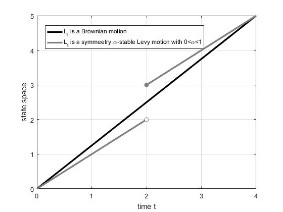
Figure 2: The most probable transition paths of Ornstein-Uhlenbeck process in Example 1 with $T_{0}=0,~{}T_{f}=4,~{}r=1,~{}X_{0}=0,~{}X_{f}=5$. We choose $t^{*}=2$ and the ‘right-continuous with left limit’ version of the most probable transition path.

Example 2.

Geometric Brownian motion

Consider a linear scalar SDE with multiplicative noise

$$dX_{t}=rX_{t}dt+\eta X_{t}dB_{t},$$

where $r$ and $\eta$ are real constants, and $X_{t}>0$, $a.s.$. Setting $Y_{t}=\ln X_{t}-(r-\frac{1}{2}\eta^{2})t$ and applying Itô formula, we obtain

$$dY_{t} =d\ln(X_{t})-(r-\frac{1}{2}\eta^{2})dt$$

$$=\frac{1}{X_{t}}dX_{t}+\frac{1}{2}(-\frac{1}{X_{t}^{2}})(dX_{t})^{2}-(r-\frac{1}{2}\eta^{2})dt$$

$$=\frac{dX_{t}}{X_{t}}-\frac{1}{2}\eta^{2}dt-(r-\frac{1}{2}\eta^{2})dt$$

$$=\eta dB_{t}.$$

By Corollary 1,

$$Y^{m}_{t}=Y_{0}+\frac{t-T_{0}}{T_{f}-T_{0}}(Y_{f}-Y_{0}).$$

Thus

$$X^{m}_{t}=\exp\{(r-\frac{1}{2}\eta^{2})t+\ln X_{0}+\frac{t-T_{0}}{T_{f}-T_{0}}[\ln X_{f}-(r-\frac{1}{2}\eta^{2})T_{f}-\ln X_{0}]\}.$$

Figure 3 shows the most probable transition path of this example.

Example 3.

Geometric Lévy process

Consider the stochastic differential equation

$$dX_{t}=X_{t}[\zeta dt+\beta dB(t)+\int_{\mathbb{R}}\gamma(t,z)\bar{N}(dt,dz)],$$

where $\zeta,~{}\beta$ are constants and $\gamma(t,z)\geq-1$, and

$$\bar{N}(dt,dz)=\begin{cases}N(dt,dz)-\nu(dz)dt,~{}if~{}|z|<r,\\ N(dt,dz),~{}if~{}|z|\geq r,\\ \end{cases}$$

$r\in\mathbb{R}+$. For simplicity we set $\beta=0,~{}\gamma(t,z)=e^{z}-1$. Now define $Y_{t}=\ln X_{t}$. By Itô formula, we have

$$dY_{t} =\zeta dt+\int_{|z|<r}\{\ln(1+e^{z}-1)-(e^{z}-1)\}\nu(dz)dt+\int_{\mathbb{R}}\ln(1+e^{z}-1)\bar{N}(dt,dz)$$

$$=\zeta dt+\int_{|z|<r}\{z-(e^{z}-1)\}\nu(dz)dt+\int_{\mathbb{R}}z\bar{N}(dt,dz).$$

Let $U_{t}=Y_{t}-(\zeta+\int_{|z|<r}\{z-(e^{z}-1)\}\nu(dz))t$ be a symmetric $\alpha$-stable Lévy process, i.e., $dU_{t}=\int_{r}z\bar{N}(dt,dz)=dL^{\alpha}_{t}$.

Let the jump measure $\nu(dz)$ be the jump measure of an $\alpha$-stable Lévy process, that is, $\nu(dz)=c_{\alpha}\frac{dz}{|z|^{1+\alpha}}$ with

$$c_{\alpha}=\frac{\alpha}{2^{1-\alpha}\sqrt{\pi}}\frac{\Gamma(\frac{1+\alpha}{2})}{\Gamma(1-\frac{\alpha}{2})}.$$

For $\alpha$ with $0<\alpha<1$ and $~{}r=1$,

$$\int_{|z|<1}\{z-(e^{z}-1)\}\nu(dz)<\infty.$$

By Corollary 1, the most probable transition path of $U_{t}$ is

$$U^{m}_{t}=\begin{cases}U_{0},~{}T_{0}\leq t<t^{*}~{}(T_{0}\leq t\leq t^{*}),\\ U_{f},~{}t^{*}\leq t\leq T_{f}~{}(t^{*}<t\leq T_{f}),\end{cases}$$

where $t^{*}\in[T_{0},T_{f}]$. Thus

$$X^{m}_{t}=\begin{cases}\exp(\ln X_{0}+(t-T_{0})[\zeta+\int_{|z|<1}\{z-(e^{z}-1)\}\nu(dz)]),~{}T_{0}\leq t<t^{*}~{}(T_{0}\leq t\leq t^{*}),\\ \exp(\ln X_{f}+(t-T_{f})[\zeta+\int_{|z|<1}\{z-(e^{z}-1)\}\nu(dz)]),~{}t^{*}\leq t\leq T_{f}~{}(t^{*}<t\leq T_{f}).\\ \end{cases}$$

Figure 3 also shows the most probable transition path of this example.

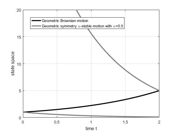
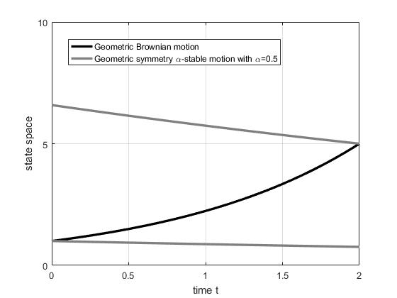
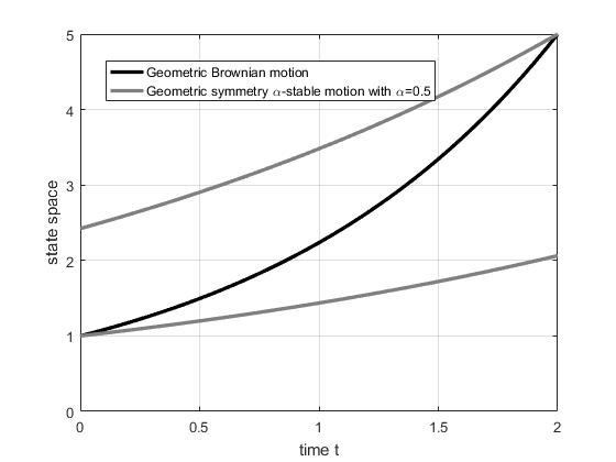
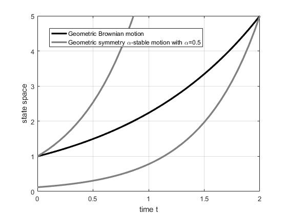
Figure 3: The most probable transition paths of Geometric Brownian motion (black solid line) and the initial and final transition path of geometry symmetric $\alpha$-stable Lévy motion with $\alpha=0.5$ (grey solid lines, the most probable path starts at initial transition path and jumps to final transition path at time $t^{*}=1$), for $T_{0}=0,~{}T_{f}=2,~{}X_{0}=1,~{}X_{2}=5,~{}r=1,~{}\eta=1,~{}\beta=0$: $(a)~{}\zeta=-1;(b)~{}\zeta=0;(c)~{}\zeta=0.5;(d)~{}\zeta=2.$

Example 4.

One-dimensional Nonlinear SDE: Stochastic double-well system

Consider the stochastic double-well system

$$dX_{t}=(X_{t}-X_{t}^{3})dt+dL_{t},$$

where $L_{t}$ is a symmetric $\alpha$-stable Lévy motion with $0<\alpha<1$.

The corresponding undisturbed system has three equilibrium points: -1, 0, 1 ( -1 and 1 are stable equilibrium points, 0 is an unstable equilibrium point).

By Theorem 2, the most probable transition path of this system is described by the following deterministic differential equation:

$$\begin{cases}dX^{m}_{t}-(X^{m}_{t}-(X^{m}_{t})^{3})dt=0,~{}t\in[T_{0},T_{f}]\backslash\{t^{*}\},\\ X^{m}_{T_{0}}=X_{0},~{}X^{m}_{T_{f}}=X_{f},~{}t^{*}\in[T_{0},T_{f}].\\ \end{cases}$$

We compute some solution curves of above system as shown in Figure 4. The most probable transition path consists of the solutions of this deterministic system. For instance, if we consider: $X_{0}=1$, $X_{f}=-1$, $T_{0}=0$, $T_{f}=4$, then the most probable transition path consists of the parts of two straight lines in Figure 4.

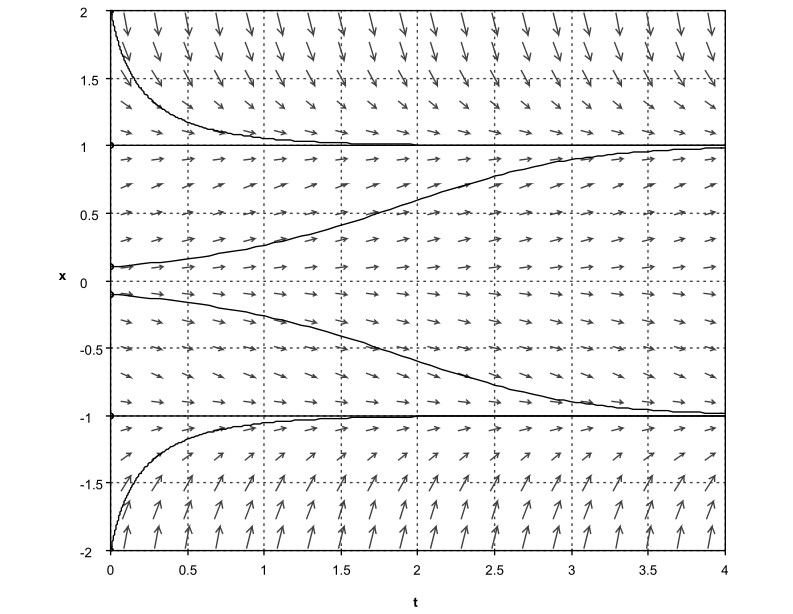
Figure 4: Solution curves for $\dot{x}=x-x^{3}$.

Example 5.

Two-Dimensional Nonlinear SDE: The Maier-Stein model

Consider the following SDEs:

$$\begin{cases}du=(u-u^{3}-\beta uv^{2})dt+dL_{1,t},\\ dv=-(1+u^{2})vdt+dL_{2,t},\end{cases}$$

By Theorem 2, the most probable transition path $(u^{m}_{t},v^{m}_{t})$ of this system is described by the following deterministic differential equations:

$$\begin{cases}du^{m}_{t}=(u^{m}_{t}-(u^{m}_{t})^{3}-\beta u^{m}_{t}(v^{m}_{t})^{2})dt,~{}t\in[T_{0},T_{f}]\backslash\{t^{*}\},\\ dv^{m}_{t}=-(1+(u^{m}_{t})^{2})v^{m}_{t}dt,~{}t\in[T_{0},T_{f}]\backslash\{t^{*}\},\\ u^{m}_{T_{0}}=u_{0},~{}u^{m}_{T_{f}}=u_{f},~{}v^{m}_{T_{0}}=v_{0},~{}v^{m}_{T_{f}}=v_{f},~{}t^{*}\in[T_{0},T_{f}].\\ \end{cases}$$

Figure 5 shows the phase portrait of this deterministic system. There are three equilibrium points: $(-1,0),(0,0),(1,0)$. In Figure 5 we show several orbits in black lines. The most probable transition path can be found by the phase portrait with given initial and terminal conditions.

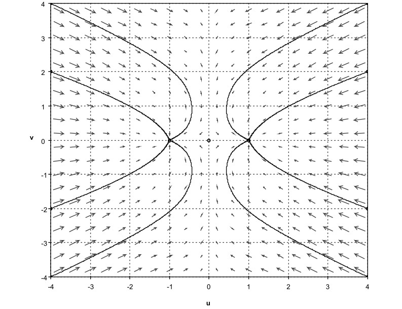
Figure 5: Phase portrait for the Maier-Stein model.

References

References

- [1] D. Dürr and A. Bach. The Onsager-Machlup Function as Lagrangian for the Most Probable Path of a Diffusion Process. Commun.Math. Phys. 60: 153 (1978).
- [2] K. L. C. Hunt, and J. Ross. Path integral solutions of stochastic equations for nonlinear irreversible processes: The uniqueness of the thermodynamic Lagrangian. The Journal of Chemical Physics. 75, 976 (1981).
- [3] S. Machlup and L. Onsager. Fluctuations and Irreversible Processes. Phys. Rev. 91, 1512 (1953).
- [4] P. Faccioli, M. Sega, F. Pederiva, and H. Orland. Dominant Pathways in Protein Folding. Phys.Rev. Lett. 97, 108101 (2006).
- [5] D. M. Zuckerman and T. B. Woolf. Efficient dynamic importance sampling of rare events in one dimension. Phys. Rev. E. 63, 016702 (2000).
- [6] J. Wang, K. Zhang, H. Lu, and E. Wang. Dominant Kinetic Paths on Biomolecular Binding-Folding Energy Landscape. Phys. Rev. Lett. 96, 168101 (2006).
- [7] G. Gobbo, A. Laio, A. Maleki, and S. Baroni. Absolute Transition Rates for Rare Events from Dynamical Decoupling of Reaction Variables. Phys. Rev. Lett. 109, 150601 (2012).
- [8] F. Langouche, D. Roekaerts and E. Tirapegui, Functional Intrgration and Semiclassical Expansions (Springer, The Netherlands) 1982.
- [9] L.S. Schulman. Techniques and Applications of Path Integration (Wiley,New York).(1981).
- [10] F.W. Wiegel. Introduction to path integral methods in physics and polymer science (World Scientific,Singapore) (1986).
- [11] H. S. Wio. Path Integrals for Stochastic Processes: An Introduction. World Scientific, New York (2013).
- [12] D.C. Khandekar, S.V. Lawande, K.V. Baghwat. Path integral methods and their applications (World Scientific, Singapore) (2000).
- [13] Y. Tang, R. Yuan, P. Ao. Summing over trajectories of stochastic dynamics with multiplicative noise. J. Chem. Phys. 141, Article 044125 (2014).
- [14] R. P. Feynman and A. R. Hibbs. Quantum Mechanics and Path Integrals (New York: McGraw-Hill) (1965).
- [15] Z. G. Arenas and D. G. Barci. Functional integral approach for multiplicative stochastic processes. Phys. Rev. E. 81, 051113 (2010).
- [16] A. W. C. Lau and T. C. Lubensky. State-dependent diffusion: Thermodynamic consistency and its path integral formulation. Phys. Rev. E. 76,011123 (2007).
- [17] H.S. Wio, Application of Path Integration to Stochastic Processes. An Introduction, chapter in. Fundamentals and Applications of Complex Systems, Ed. G. Zgrablich, (Nueva Edit. Univ., Univ.Nac. San Luis), pg. 253. (1999).
- [18] N. Laskin. Fractional quantum mechanics. Phys. Rev. E. 66, 056108 (2002).
- [19] D. Janakiraman and K. L. Sebastian, Path-integral formulation for L vy flights: Evaluation of the propagator for free, linear, and harmonic potentials in the over- and underdamped limits, Phys. Rev. E. 86, 061105 (2012).
- [20] D. Applebaum. L vy Processes and Stochastic Calculus (Cambridge: Cambridge University Press) (2009).
- [21] K.-I. Sato. L vy Processes and Infinite Divisibility. Cambridge University Press (1999).
- [22] N. Jacob, V. Knopova, S. Landwehr, and R. Schilling. A geometric interpretation of the transition density of a symmetric Lévy process. Sci. China Math. 55(6): 1099 C1126 (2012).
- [23] N. Jacob. Pseudo-Differential Operators and Markov Processes, vol.1: Fourier Analysis and Semigroups. London: Imperial College Press (2001).
- [24] J. Duan. An Introduction to Stochastic Dynamics (New York: Cambridge University Press) (2015).
- [25] A. Janicki and A. Weron. Simulation and Chaotic Behavior of alpha-Stable Stochastic Processes. New York: Marcel Dekker (1994).
- [26] M. Shao and C. L. Nikias. Signal processing with fractional lower order moments: Stable processes and their applications. Proc. of the IEEE. 81(7): 986-1010 (1993).
- [27] S. Albeverio, Z. Brzezniak and J. Wu. Existence of global solutions and invariant measures for stochastic differential equations driven by poisson type noise with non-lipschitz coefficients Journal of Mathematical Analysis and Applications. 371(1) 309-322 (2010).
- [28] F. Xi, C. Zhu. Jump type stochastic differential equations with non-Lipschitz coefficients: Non-confluence, Feller and strong Feller properties, and exponential ergodicity. J. Differential Equations(2018), https://doi.org/10.1016/j.jde.2018.10.006.
- [29] R. B. Ash. Probability and Measure Theory (A Harcourt Science and Technology Company press) (1999).
- [30] M. Delarue, P. Koehl, and H. Orland. Ab initio sampling of transition paths byconditioned Langevin dynamics. J. Chem. Phys. 147, 152703 (2017).
- [31] Y. Zheng and X. Sun. Governing equations for Probability densities of stochastic differential equations with discrete time delays. Discrete & Continuous Dynamical Systems-B. 22 (9) : 3615-3628. (2017).
- [32] Z. G. Arenas and D. G. Barci. Hidden symmetries and equilibrium properties of multiplicative white-noise stochastic processes. J. Stat. Mech. P12005 (2012)
- [33] M. V. Moreno, Z. G. Arenas, and D. G. Barci. Langevin dynamics for vector variables driven by multiplicative white noise: A functional formalism. Phys. Rev. E. 91, 042103 (2015).