Gauge field theories with Lorentz-violating operators of arbitrary dimension

Abstract

The classification of Lorentz- and CPT-violating operators in nonabelian gauge field theories is performed. We construct all gauge-invariant terms describing propagation and interaction in the action for fermions and gauge fields. Restrictions to the abelian, Lorentz-invariant, and isotropic limits are presented. We provide two illustrative applications of the results to quantum electrodynamics and quantum chromodynamics. First constraints on nonlinear Lorentz-violating effects in electrodynamics are obtained using data from experiments on photon-photon scattering, and corrections from nonminimal Lorentz and CPT violation to the cross section for deep inelastic scattering are derived.

I Introduction

Nonabelian gauge theories, introduced by Yang and Mills in 1954 ym54 , play a central role in physics. Applications to particle physics such as the Standard Model (SM) typically combine nonabelian gauge invariance with the foundational Lorentz symmetry of relativity. In recent years, however, attention has been drawn to the possibility that tiny violations of Lorentz symmetry could arise in a unified theory of gravity and quantum physics such as strings ksp , triggering many searches for potentially observable signals in laboratory experiments and astrophysical observations tables . Studies of Lorentz-violating nonabelian gauge theories are therefore of immediate interest in the phenomenological context.

Using effective field theory sw , a realistic and comprehensive description of Lorentz violation encompassing the nonabelian gauge symmetry of the SM can be developed. This approach starts with the SM action coupled to General Relativity (GR) and adds all coordinate-independent terms formed as the contraction of a Lorentz-violating operator with a coefficient governing the size of its physical effects. The resulting framework is called the Standard-Model Extension (SME) ck ; ak04 . The SME also provides a general description of CPT violation in realistic field theory because CPT invariance follows from Lorentz invariance in effective field theory ck ; owg .

In Minkowski spacetime, the SME is a Lorentz-violating nonabelian gauge theory based on the gauge group SU(3)$\times$SU(2)$\times$U(1). The subset of terms constructed from operators with mass dimensions $d\leq 4$ forms the minimal SME, which is power-counting renormalizable. In a scenario with the SM and GR emerging as the low-energy limit of a unified theory of quantum physics and gravity, operators with smaller $d$ can be expected to dominate the low-energy Lorentz-violating physics. The experimental viability of any specific Lorentz-violating model compatible with realistic effective field theory can be determined by matching the model parameters to the corresponding subset of SME coefficients and their known experimental bounds tables ; reviews .

Most treatments of Lorentz violation to date emphasize effects in the minimal SME. For the nonminimal sector, a complete enumeration exists of operators at arbitrary $d$ that modify the gauge-invariant propagation of various particle species, including scalars, Dirac fermions, neutrinos, photons, and gravitons km ; ek18 . However, much less is known about the general form of gauge-invariant interactions at arbitrary $d$. In particular, no general treatment of the nonabelian case exists to date, although a few works consider special nonminimal nonabelian Lorentz-violating operators bp08 ; ar14 ; em14 ; jc15 ; em16 ; nvt16 ; mf17 ; mfm18 . Even in the comparatively simple case of Lorentz-violating quantum electrodynamics (QED), only a subset of interactions for $d\leq 6$ has been systematically classified dk16 .

The focus of the present work is closing this gap in the literature. We exhibit here a construction of Lorentz-violating terms at arbitrary $d$ in the Lagrange density for a generic nonabelian gauge field theory with fermion couplings. The case of Lorentz-violating QED emerges as the abelian limit of this theory. For definiteness, we assume here a Minkowski background spacetime and an action invariant both under a nonabelian gauge group and under spacetime translations, thereby insuring conservation of energy and momentum. This setup generates a framework appropriate for many experimental applications, as we illustrate below with examples drawn from Lorentz-violating QED and from the theory of Lorentz-violating quantum chromodynamics (QCD) and QED coupled to quarks. The operators constructed here are potentially of formal theoretical importance in contexts such as studies of causality and stability causality and the recently uncovered links to Riemann-Finsler geometry ek18 ; finsler . They also offer prospective applications to searches for Lorentz-invariant geometric forces extending GR such as torsion torsion and nonmetricity nonmetricity , as well as to studies of phenomenological Lorentz-violating scenarios focusing on operators with $d>4$ such as supersymmetric models susy and noncommutative quantum field theories ncqft .

This work is organized as follows. In Sec. II, we demonstrate that any gauge-covariant combination of covariant derivatives and gauge-field strengths can be expressed in a standard form, and we derive some useful properties. The general nonabelian gauge field theory including Lorentz and CPT violation is constructed in Sec. III. We present in turn the fermion sector, the pure-gauge sector, and the fermion-gauge sector of this theory, providing in tabular form the explicit expressions for all operators of mass dimension $d\leq 6$. This section also considers several limits of interest, including Lorentz-violating QED, Lorentz-violating QCD and QED, the Lorentz-invariant restriction, and the isotropic case.

Two experimental applications of the results are considered in Sec. IV. One is the effect on light-by-light scattering of certain nonminimal operators in Lorentz-violating QED. Data from an experiment at the Large Hadron Collider (LHC) are used to obtain first constraints on some coefficients for Lorentz violation. The second application is to deep inelastic scattering (DIS). Corrections to the cross section for electron-proton scattering arising from certain nonminimal Lorentz- and CPT-violating operators are obtained. Throughout this work, our conventions follow those of Ref. km . In particular, the Minkowski metric $\eta_{\mu\nu}$ has negative signature, and the Levi-Civita tensor $\epsilon^{\kappa\lambda\mu\nu}$ is defined with $\epsilon^{0123}=+1$.

II Gauge-covariant operators

One goal of this work is to classify and enumerate all terms in the Lagrange density for a Lorentz- and CPT-violating nonabelian gauge theory. For this purpose, it is useful first to establish a standard basis spanning the space of all gauge-covariant operators. A generic term in the Lagrange density can then be decomposed in terms of the standard basis. In this section, we identify a suitable standard basis and establish some of its properties.

II.1 Setup

Consider a gauge field theory of a Dirac fermion $\psi$ taking values in a specific representation $U$ of the gauge group ${\cal G}$. Assuming ${\cal G}$ is a compact Lie group, a suitable inner product can be chosen to make the representation unitary ms07 , $UU^{\dagger}=U^{\dagger}U=1$. Under a gauge transformation, $\psi$ transforms covariantly by construction, $\psi\to U\psi$, while its Dirac conjugate $\overline{\psi}{}\equiv\psi^{\dagger}\gamma^{0}$ transforms as $\overline{\psi}{}\to\overline{\psi}{}U^{\dagger}$.

Acting on $\psi$, the gauge-covariant derivative can be written as $D_{\mu}\psi=\partial_{\mu}\psi-igA_{\mu}\psi$, where $g$ is the gauge coupling constant and $A_{\mu}$ is the gauge field in the $U$ representation. Since $U$ is unitary, $A_{\mu}$ is hermitian. By definition, the covariant derivative satisfies $D_{\mu}\to UD_{\mu}U^{\dagger}$ under a gauge transformation, and so the gauge field obeys $A_{\mu}\to UA_{\mu}U^{\dagger}+(i/g)U\partial_{\mu}U^{\dagger}$.

The commutator of two covariant derivatives acting on $\psi$ generates the gauge-field strength $F_{\mu\nu}$ in the $U$ representation, ${[D_{\mu},D_{\nu}]}\psi=-igF_{\mu\nu}\psi$. Like $A_{\mu}$, $F_{\mu\nu}$ is hermitian. Under a gauge transformation, $F_{\mu\nu}\to UF_{\mu\nu}U^{\dagger}$. The action of the covariant derivative on the field strength is $D_{\mu}F_{\beta\gamma}=\partial_{\mu}F_{\beta\gamma}-ig[A_{\mu},F_{\beta\gamma}]$, while the product of two covariant derivatives acting on the field strength obeys $D_{\mu}(D_{\nu}F_{\beta\gamma})-D_{\nu}(D_{\mu}F_{\beta\gamma})=-ig[F_{\mu\nu},F_{\beta\gamma}]$.

The above results imply that a gauge transformation on single covariant derivatives of the fields yields $D_{\mu}\psi\to U(D_{\mu}\psi)$ and $\overline{D_{\mu}\psi}\to(\overline{D_{\mu}\psi})U^{\dagger}$ for fermions, along with $D_{\mu}F_{\beta\gamma}\to U(D_{\mu}F_{\beta\gamma})U^{\dagger}$ for the gauge-field strength. By induction, we can prove that multiple covariant derivatives on each field transform according to

$$D_{\alpha_{1}}\!\cdots\!D_{\alpha_{n}}\psi \to U(D_{\alpha_{1}}\!\cdots\!D_{\alpha_{n}}\psi),$$

$$\overline{D_{\alpha_{1}}\!\cdots\!D_{\alpha_{n}}\psi} \to (\overline{D_{\alpha_{1}}\!\cdots\!D_{\alpha_{n}}\psi})U^{\dagger},$$

$$D_{\alpha_{1}}\!\cdots\!D_{\alpha_{n}}F_{\beta\gamma} \to U(D_{\alpha_{1}}\!\cdots\!D_{\alpha_{n}}F_{\beta\gamma})U^{\dagger}.$$ (1)

It is convenient to call an operator ${\cal O}$ a gauge-covariant operator if ${\cal O}\to U{\cal O}U^{\dagger}$ under a gauge transformation. Gauge-covariant operators are of interest in the present context because they can be used to construct gauge-invariant terms such as $\textrm{tr}({\cal O})$ and $(\overline{{\cal O}_{1}\psi}){\cal O}_{2}\psi$, which are therefore candidates for inclusion in the general Lagrange density for the Lorentz-violating gauge field theory. In particular, we see that any operator ${\cal O}$ formed as a mixture of $D$ and $F$ is gauge covariant.

II.2 Result

In principle, one could construct the desired general Lagrange density for a Lorentz- and CPT-violating gauge field theory by adding all possible gauge-invariant operators to the usual minimal-coupling terms. However, this procedure would introduce substantial redundancies due to relations among the gauge-invariant operators. Instead, we can characterize gauge-covariant operators in terms of a standard basis set, which can then be used to construct the Lagrange density with controlled or no redundancy.

The key result is that the gauge-covariant operators formed as any mixture of $D$ and $F$ can be expressed as a linear combination of operators of the standard form

$$(D_{(n_{1})}F_{\mu_{1}\nu_{1}})(D_{(n_{2})}F_{\mu_{2}\nu_{2}})\cdots(D_{(n_{m})}F_{\mu_{m}\nu_{m}})D_{(n_{m+1})},$$ (2)

where $D_{(n)}=(1/n!)\sum D_{\alpha_{1}}D_{\alpha_{2}}\!\cdots\!D_{\alpha_{n}}$ with the summation performed over all permutations of $\alpha_{1},\alpha_{2},\cdots\alpha_{n}$. In what follows, we prove this result and present some of its properties.

II.2.1 Proof

For the proof, we suppose that the operator (2) acts on $\psi$. An analogous argument applies for the case where the operator acts on $F$ instead.

Given a gauge-covariant operator ${\cal O}$ formed as an arbitrary mixture of $D$ and $F$, we first use standard product rules like $D_{\mu}F_{\alpha\beta}D_{\nu}=(D_{\mu}F_{\alpha\beta})D_{\nu}+F_{\alpha\beta}D_{\mu}D_{\nu}$ to express it as a linear combination of terms in the block form

$${\cal O}=\sum(DD\cdots DF)\cdots(DD\cdots DF)DD\cdots D,$$ (3)

where all subscripts are omitted for simplicity. Each covariant derivative $D$ then acts on at most one field strength $F$. To prove the main result, it therefore suffices to show that terms like $D_{\alpha_{1}}D_{\alpha_{2}}\cdots D_{\alpha_{n}}$ can be expressed as linear combinations of the form (2).

We use mathematical induction. For $n=1$, $D_{\alpha_{1}}$ already takes the form (2). Assume that for $n\leq k$ the term $D_{\alpha_{1}}D_{\alpha_{2}}\cdots D_{\alpha_{n}}$ can be written as a linear combination of terms having the form (2). Then, for $n=k+1$ we must consider $D_{\alpha_{1}}D_{\alpha_{2}}\cdots D_{\alpha_{k}}D_{\alpha_{k+1}}$. Replacing the first $k$ derivatives by the appropriate linear combination of terms having the form (2) yields expressions with the structure $(D_{(n_{1})}F_{\beta_{1}\gamma_{1}})\cdots D_{(n_{m+1})}D_{\alpha_{k+1}}$. This shows that it suffices to focus only on the term $D_{(n_{m+1})}D_{\alpha_{k+1}}$.

If $n_{m+1}\leq k-1$, then we get at most $k$ covariant derivatives. By induction, all such terms can be written as a linear combination of terms having the form (2).

For $n_{m+1}=k$, we must consider $D_{(k)}D_{\alpha_{k+1}}$. The index symmetries of this product can be displayed using Young tableaux,

$$\psset{unit=12.0pt,linewidth=0.5pt}\begin{pspicture}[missing](48.0pt,12.0pt)\small{\psline(0.0pt,0.0pt)(0.0pt,12.0pt)(48.0pt,12.0pt)}{\psline(0.0pt,0.0pt)(12.0pt,0.0pt)(12.0pt,12.0pt)}\rput(0.0pt,0.0pt){\rput(6.0pt,6.0pt){$\scriptstyle 1$}}{\psline(12.0pt,0.0pt)(24.0pt,0.0pt)(24.0pt,12.0pt)}\rput(12.0pt,0.0pt){\rput(6.0pt,6.0pt){$\scriptstyle 2$}}{\psline(24.0pt,0.0pt)(36.0pt,0.0pt)(36.0pt,12.0pt)}\rput(24.0pt,0.0pt){\rput(6.0pt,6.0pt){$\scriptstyle\cdots$}}{\psline(36.0pt,0.0pt)(48.0pt,0.0pt)(48.0pt,12.0pt)}\rput(36.0pt,0.0pt){\rput(6.0pt,6.0pt){$\scriptstyle k$}}\end{pspicture}\otimes\psset{unit=12.0pt,linewidth=0.5pt}\begin{pspicture}[missing](12.0pt,12.0pt)\small{\psline(0.0pt,0.0pt)(0.0pt,12.0pt)(12.0pt,12.0pt)}{\psline(0.0pt,0.0pt)(12.0pt,0.0pt)(12.0pt,12.0pt)}\rput(0.0pt,0.0pt){\rput(6.0pt,6.0pt){$\scriptstyle k\!+\!1$}}\end{pspicture}=\psset{unit=12.0pt,linewidth=0.5pt}\begin{pspicture}[missing](60.0pt,12.0pt)\small{\psline(0.0pt,0.0pt)(0.0pt,12.0pt)(60.0pt,12.0pt)}{\psline(0.0pt,0.0pt)(12.0pt,0.0pt)(12.0pt,12.0pt)}\rput(0.0pt,0.0pt){\rput(6.0pt,6.0pt){$\scriptstyle 1$}}{\psline(12.0pt,0.0pt)(24.0pt,0.0pt)(24.0pt,12.0pt)}\rput(12.0pt,0.0pt){\rput(6.0pt,6.0pt){$\scriptstyle 2$}}{\psline(24.0pt,0.0pt)(36.0pt,0.0pt)(36.0pt,12.0pt)}\rput(24.0pt,0.0pt){\rput(6.0pt,6.0pt){$\scriptstyle\cdots$}}{\psline(36.0pt,0.0pt)(48.0pt,0.0pt)(48.0pt,12.0pt)}\rput(36.0pt,0.0pt){\rput(6.0pt,6.0pt){$\scriptstyle k$}}{\psline(48.0pt,0.0pt)(60.0pt,0.0pt)(60.0pt,12.0pt)}\rput(48.0pt,0.0pt){\rput(6.0pt,6.0pt){$\scriptstyle k\!+\!1$}}\end{pspicture}\oplus\psset{unit=12.0pt,linewidth=0.5pt}\begin{pspicture}[missing](48.0pt,24.0pt)\small{\psline(0.0pt,0.0pt)(0.0pt,24.0pt)(48.0pt,24.0pt)}{\psline(0.0pt,12.0pt)(12.0pt,12.0pt)(12.0pt,24.0pt)}\rput(0.0pt,12.0pt){\rput(6.0pt,6.0pt){$\scriptstyle 1$}}{\psline(12.0pt,12.0pt)(24.0pt,12.0pt)(24.0pt,24.0pt)}\rput(12.0pt,12.0pt){\rput(6.0pt,6.0pt){$\scriptstyle 2$}}{\psline(24.0pt,12.0pt)(36.0pt,12.0pt)(36.0pt,24.0pt)}\rput(24.0pt,12.0pt){\rput(6.0pt,6.0pt){$\scriptstyle\cdots$}}{\psline(36.0pt,12.0pt)(48.0pt,12.0pt)(48.0pt,24.0pt)}\rput(36.0pt,12.0pt){\rput(6.0pt,6.0pt){$\scriptstyle k$}}{\psline(0.0pt,0.0pt)(12.0pt,0.0pt)(12.0pt,12.0pt)}\rput(0.0pt,0.0pt){\rput(6.0pt,6.0pt){$\scriptstyle k\!+\!1$}}\end{pspicture}.$$ (4)

The first Young tableau on the right-hand side represents $D_{(k+1)}$, which has the claimed form. We can therefore limit further consideration to the second Young tableau.

We can prove that the expression involving the second Young tableau contains least one factor of the field strength $F$. Explicitly, we can write this expression in the form

$$\hskip-30.0ptD_{(\alpha_{1}}D_{\alpha_{2}}\cdots D_{\alpha_{k})}D_{\alpha_{k+1}}-D_{(\alpha_{k+1}}D_{\alpha_{2}}\cdots D_{\alpha_{k})}D_{\alpha_{1}}$$

$$\hskip 20.0pt=\frac{2}{k}\sum_{t=0}^{k-1}D_{(t)}D_{[\alpha_{1}}D_{(k-t-1)}D_{\alpha_{k+1}]},$$ (5)

where the parentheses around indices indicate symmetrization with a factor of $1/k!$ and the brackets indicate antisymmetrization on $\alpha_{1}$ and $\alpha_{k+1}$ with a factor of $1/2$. Note that this result is symmetric under the interchange of the indices in $D_{(t)}$ with those in $D_{(k-t-1)}$.

A specific term inside the sum in Eq. (5) takes the form

$$D_{(t)}D_{[\alpha_{1}}D_{(k-t-1)}D_{\alpha_{k+1}]} = D_{(t)}D_{[\alpha_{1}}D_{\alpha_{k+1}]}D_{(k-t-1)}$$

$$+D_{(t)}D_{[\alpha_{1}}[D_{(k-t-1)},D_{\alpha_{k+1}]}].$$

The first term on the right-hand side involves $[D_{\alpha_{1}},D_{\alpha_{k+1}}]=-igF_{\alpha_{1}\alpha_{k+1}}$, thus confirming the appearance of a factor of $F$. For the second term, we note that

$$\hskip-20.0ptD_{(t)}D_{\alpha_{1}}[D_{(k-t-1)},D_{\alpha_{k+1}}]$$

$$= \tfrac{1}{(k-t-1)!}\sum D_{(t)}D_{\alpha_{1}}[D_{\beta_{1}}D_{\beta_{2}}\cdots D_{\beta_{k-t-1}},D_{\alpha_{k+1}}]$$

$$= \tfrac{1}{(k-t-1)!}\sum D_{(t)}D_{\alpha_{1}}\big{(}D_{\beta_{1}}[D_{\beta_{2}}\cdots D_{\beta_{k-t-1}},D_{\alpha_{k+1}}]$$

$$\hskip 50.0pt+[D_{\beta_{1}},D_{\alpha_{k+1}}]D_{\beta_{2}}\cdots D_{\beta_{k-t-1}}\big{)}$$

$$= \tfrac{1}{(k-t-1)!}\sum\big{(}D_{(t)}D_{\alpha_{1}}D_{\beta_{1}}[D_{\beta_{2}}\cdots D_{\beta_{k-t-1}},D_{\alpha_{k+1}}]$$

$$\hskip 50.0pt-igD_{(t)}D_{\alpha_{1}}F_{\beta_{1}\alpha_{k+1}}D_{\beta_{2}}\cdots D_{\beta_{k-t-1}}\big{)},$$

where the summations are over all permutations of $\beta_{1},\beta_{2},\cdots\beta_{k-t-1}$. Continuing this reductive process yields a string of terms, each of which contains one factor of $F_{\mu\nu}$ along with $(k-1)$ covariant derivatives. Therefore, every term in the expression for the second Young tableau in Eq. (5) involves at least one field strength $F$. Each such term has the general form $D_{\gamma_{1}}\cdots D_{\gamma_{s}}F_{\mu\nu}D_{\gamma_{s+1}}\cdots D_{\gamma_{k-1}}$. Using product rules as before, we can transform this into the block form (3). In each block, we have at most $k-1\leq k$ covariant derivatives. By the induction assumption, these terms can all be written as linear combinations having the form (2). This completes the induction step and proves the claimed result.

II.2.2 Linear independence

The above argument shows that the basis (2) of gauge-covariant operators is complete, but it leaves open the question of linear independence. The situation in this respect can differ depending on whether the group ${\cal G}$ is abelian or nonabelian.

Consider first an abelian gauge field theory, for which $D_{(n)}F_{\beta\gamma}=\partial_{(n)}F_{\beta\gamma}$. Note that $\partial_{(n_{1})}F_{\beta_{1}\gamma_{1}}$ commutes with $\partial_{(n_{2})}F_{\beta_{2}\gamma_{2}}$ and also that the operators $\{\partial_{(n)}F_{\beta\gamma}\}$ are linearly independent for different $n$. A complete set of linearly independent basis operators can therefore be selected as

$$\{(\partial_{(n_{1})}F_{\beta_{1}\gamma_{1}})\cdots(\partial_{(n_{t})}F_{\beta_{t}\gamma_{t}})D_{(n_{t+1})}|n_{1}\leq\cdots\leq n_{t}\}.$$ (8)

This set can be used to classify all gauge-covariant operators formed from mixtures of $D$ and $F$ in QED, in a manner free of redundancy.

For a nonabelian group, the noncommutativity of products of the field strength $F$ implies that gauge-covariant operators having the form (2) are generically linearly independent. When ${\cal G}$ is SU(2), for example, the three generators of ${\cal G}$ are mutually noncommutative, implying that basis elements of the form (2) are linearly independent.

However, if a nonabelian ${\cal G}$ has an abelian Lie subgroup of dimension two or more, the choice of linearly independent basis becomes more intricate. In QCD, for example, $U$ is the vector representation of the gauge group SU(3), which has a subgroup U(1)$\times$U(1) homomorphic to the torus $T^{2}$. This subgroup is spanned by 3$\times$3 commuting matrices with diagonal elements of the form $\{e^{i\theta_{1}},e^{i\theta_{2}},e^{-i(\theta_{1}+\theta_{2})}\}$. Gauge-covariant operators for basis elements in U(1)$\times$U(1) can therefore be taken to have the form (8), while other basis elements are of the form (2). This shows that in a nonabelian gauge field theory the selection of a basis for the gauge-covariant operators depends on the gauge group. For simplicity in what follows, we adopt basis elements of the form (2) for nonabelian gauge field theory and tolerate any ensuing partial redundancy.

II.2.3 Hermitian conjugation

For some of the applications to follow, it is useful to have explicit expressions for the hermitian conjugates of the component terms in the gauge-covariant operators (2) and of general fermion bilinears. We obtain these next.

First, we prove the identity

$$(D_{(n)}F_{\beta\gamma})^{\dagger}=D_{(n)}F_{\beta\gamma}.$$ (9)

To begin, use direct calculation to show $(D_{\alpha}F_{\beta\gamma})^{\dagger}=D_{\alpha}F_{\beta\gamma}$. We can then use mathematical induction to show that $(D_{\alpha_{1}}\!\cdots\!D_{\alpha_{n}}F_{\beta\gamma})^{\dagger}=D_{\alpha_{1}}\!\cdots\!D_{\alpha_{n}}F_{\beta\gamma}$ for any $n$, as follows. The result is true for $n=1$. Assuming it holds for $n=k$, we find

$$\hskip-30.0pt(D_{\alpha}D_{\alpha_{1}}\!\cdots\!D_{\alpha_{k}}F_{\beta\gamma})^{\dagger}$$ (10)

$$= \partial_{\alpha}D_{\alpha_{1}}\!\cdots\!D_{\alpha_{k}}F_{\beta\gamma}+ig[D_{\alpha_{1}}\!\cdots\!D_{\alpha_{k}}F_{\beta\gamma},A_{\alpha}]$$

$$= D_{\alpha}D_{\alpha_{1}}\!\cdots\!D_{\alpha_{k}}F_{\beta\gamma}.$$

The result therefore also holds for $n=k+1$, as required. The desired identity (9) then follows by symmetrization on indices.

For conjugation of expressions involving fermions, two results are useful. For one, the identity (9) directly implies

$$\overline{(D_{(n)}F_{\beta\gamma})\psi}=\overline{\psi}{}(D_{(n)}F_{\beta\gamma}).$$ (11)

The other identity involves hermitian conjugation of a general gauge-invariant bilinear of the form $(\overline{{\cal O}_{1}\psi})\Gamma_{I}({\cal O}_{2}\psi)$, where ${\cal O}_{1}$ and ${\cal O}_{2}$ are gauge-covariant operators and the spinor space is spanned by the 16 matrices $\Gamma_{I}\in\{1,i\gamma_{5},\gamma_{\mu},\gamma_{5}\gamma_{\mu},\sigma_{\mu\nu}/2\}$. Following the argument in Sec. II.2, we can choose ${\cal O}_{1}$ and ${\cal O}_{2}$ to have the form (2) and thereby write the general bilinear as

$$(\overline{D_{(n_{0})}\psi})\Gamma_{I}(D_{(n_{1})}F_{\beta_{1}\gamma_{1}})\cdots(D_{(n_{m})}F_{\beta_{m}\gamma_{m}})(D_{(n_{m+1})}\psi).$$ (12)

To find the hermitian conjugate of the bilinear (12), note that $(D_{\mu}\psi)^{\dagger}=(\overline{D_{\mu}\psi})\gamma_{0}$ and $(\overline{D_{\mu}\psi})^{\dagger}=\gamma_{0}(D_{\mu}\psi)$. In analogy with the proof of the identity (9), we can use mathematical induction to show the two results $(D_{(n)}\psi)^{\dagger}=(\overline{D_{(n)}\psi})\gamma_{0}$ and $(\overline{D_{(n)}\psi})^{\dagger}=\gamma_{0}(D_{(n)}\psi)$. Recalling the relation $\Gamma_{I}=\gamma_{0}\Gamma_{I}^{\dagger}\gamma_{0}$, we finally arrive at the elegant conjugation identity

$$\hskip-12.0pt[(\overline{D_{(n_{0})}\psi})\Gamma_{I}(D_{(n_{1})}F_{\beta_{1}\gamma_{1}})\!\cdots\!(D_{(n_{m})}F_{\beta_{m}\gamma_{m}})(D_{(n_{m+1})}\psi)]^{\dagger}$$

$$= (\overline{D_{(n_{m+1})}\psi})\Gamma_{I}(D_{(n_{m})}F_{\beta_{m}\gamma_{m}})\!\cdots\!(D_{(n_{1})}F_{\beta_{1}\gamma_{1}})(D_{(n_{0})}\psi).$$

III Gauge Field Theory

To construct the general gauge-invariant theory including Lorentz and CPT violation, it is convenient to separate the full Lagrange density ${\cal L}$ into three parts,

$${\cal L}={\cal L}_{\psi}+{\cal L}_{A}+{\cal L}^{\prime},$$ (14)

where ${\cal L}_{\psi}$ denotes the fermion sector including covariant-derivative couplings, ${\cal L}_{A}$ denotes the pure-gauge sector, and ${\cal L}^{\prime}$ is a fermion-gauge sector containing products of operators appearing in the first two parts. In this section, each of these pieces of ${\cal L}$ are considered in turn. We offer some observations about the general situation and provide explicit expressions for terms of low mass dimensionality.

III.1 Fermion sector

For a Dirac fermion, the general gauge-invariant Lagrange density ${\cal L}_{\psi}$ involving self interactions and gauge interactions via covariant derivatives can be expanded in a series of the schematic form

$${\cal L}_{\psi} = {\textstyle{\frac{1}{2}}}\overline{\psi}{}(D_{\mu}\gamma^{\mu}-m)\psi+\textrm{h.c.}$$ (15)

$$+\overline{\psi}{}\widehat{Q}\psi+\textrm{h.c.}$$

$$+(\overline{\psi}{}\widehat{Q}_{1}\psi)\big{(}(\overline{D_{(m_{1})}\psi})\widehat{Q}_{2}\psi\big{)}+\textrm{h.c.}$$

$$+(\overline{\psi}{}\widehat{Q}_{3}\psi)\big{(}(\overline{D_{(m_{2})}\psi})\widehat{Q}_{4}\psi\big{)}\big{(}(\overline{D_{(m_{3})}\psi})\widehat{Q}_{5}\psi\big{)}+\textrm{h.c.}$$

$$+\cdots,$$

where $\widehat{Q}$, $\widehat{Q}_{1}$, $\widehat{Q}_{2}$, $\cdots$ are understood to be gauge-covariant operators. Adopting the results in Sec. II, each of these operators can be expressed as a linear combination of operators of the form

$$\Gamma_{I}(D_{(n_{1})}F_{\beta_{1}\gamma_{1}})\cdots(D_{(n_{m})}F_{\beta_{m}\gamma_{m}})D_{(n_{m+1})}.$$ (16)

For brevity, the expression (15) for ${\cal L}_{\psi}$ omits spacetime indices in all but the conventional Dirac term and also omits all coefficients for Lorentz violation. It is understood that each term in ${\cal L}_{\psi}$ comes with a coefficient having spacetime indices contracted with all free spacetime indices on the total operator for that term, thereby maintaining observer Lorentz symmetry of the theory ck . Note also that no derivative $D_{(n)}$ acts on $\overline{\psi}{}$ in the first bilinear of each unconventional term in ${\cal L}_{\psi}$. Any terms with these derivatives are equivalent to the displayed ones via partial integration, modulo possible surface terms in the action.

Table 1: Terms of low mass dimension $d\leq 6$ in the fermion Lagrange density ${\cal L}_{\psi}$.

Component	Expression
${\cal L}_{\psi 0}$	${\textstyle{\frac{1}{2}}}\overline{\psi}{}(\gamma^{\mu}iD_{\mu}-m_{\psi})\psi+\textrm{h.c.}$
${\cal L}^{(3)}_{\psi}$	$-im_{5}\overline{\psi}{}\gamma_{5}\psi-a^{\mu}\overline{\psi}{}\gamma_{\mu}\psi-b^{\mu}\overline{\psi}{}\gamma_{5}\gamma_{\mu}\psi-{\textstyle{\frac{1}{2}}}H^{\mu\nu}\overline{\psi}{}\sigma_{\mu\nu}\psi$
${\cal L}^{(4)}_{\psi}$	${\textstyle{\frac{1}{2}}}c^{\mu\alpha}\overline{\psi}{}\gamma_{\mu}iD_{\alpha}\psi+{\textstyle{\frac{1}{2}}}d^{\mu\alpha}\overline{\psi}{}\gamma_{5}\gamma_{\mu}iD_{\alpha}\psi+{\textstyle{\frac{1}{2}}}e^{\alpha}\overline{\psi}{}iD_{\alpha}\psi+{\textstyle{\frac{1}{2}}}if^{\alpha}\overline{\psi}{}\gamma_{5}iD_{\alpha}\psi+{\textstyle{\frac{1}{4}}}g^{\mu\nu\alpha}\overline{\psi}{}\sigma_{\mu\nu}iD_{\alpha}\psi+\textrm{h.c.}$
${\cal L}_{\psi D}^{(5)}$	$-{\textstyle{\frac{1}{2}}}m^{(5)\alpha\beta}\overline{\psi}{}iD_{(\alpha}iD_{\beta)}\psi-{\textstyle{\frac{1}{2}}}im_{5}^{(5)\alpha\beta}\overline{\psi}{}\gamma_{5}iD_{(\alpha}iD_{\beta)}\psi$
	$-{\textstyle{\frac{1}{2}}}a^{(5)\mu\alpha\beta}\overline{\psi}{}\gamma_{\mu}iD_{(\alpha}iD_{\beta)}\psi-{\textstyle{\frac{1}{2}}}b^{(5)\mu\alpha\beta}\overline{\psi}{}\gamma_{5}\gamma_{\mu}iD_{(\alpha}iD_{\beta)}\psi-{\textstyle{\frac{1}{4}}}H^{(5)\mu\nu\alpha\beta}\overline{\psi}{}\sigma_{\mu\nu}iD_{(\alpha}iD_{\beta)}\psi+\textrm{h.c.}$
${\cal L}_{\psi F}^{(5)}$	$-{\textstyle{\frac{1}{2}}}m_{F}^{(5)\alpha\beta}\overline{\psi}{}F_{\alpha\beta}\psi-{\textstyle{\frac{1}{2}}}im_{5F}^{(5)\alpha\beta}\overline{\psi}{}\gamma_{5}F_{\alpha\beta}\psi-{\textstyle{\frac{1}{2}}}a_{F}^{(5)\mu\alpha\beta}\overline{\psi}{}\gamma_{\mu}F_{\alpha\beta}\psi-{\textstyle{\frac{1}{2}}}b_{F}^{(5)\mu\alpha\beta}\overline{\psi}{}\gamma_{5}\gamma_{\mu}F_{\alpha\beta}\psi-{\textstyle{\frac{1}{4}}}H_{F}^{(5)\mu\nu\alpha\beta}\overline{\psi}{}\sigma_{\mu\nu}F_{\alpha\beta}\psi$
${\cal L}_{\psi D}^{(6)}$	${\textstyle{\frac{1}{2}}}c^{(6)\mu\alpha\beta\gamma}\overline{\psi}{}\gamma_{\mu}iD_{(\alpha}iD_{\beta}iD_{\gamma)}\psi+{\textstyle{\frac{1}{2}}}d^{(6)\mu\alpha\beta\gamma}\overline{\psi}{}\gamma_{5}\gamma_{\mu}iD_{(\alpha}iD_{\beta}iD_{\gamma)}\psi$
	$+{\textstyle{\frac{1}{2}}}e^{(6)\alpha\beta\gamma}\overline{\psi}{}iD_{(\alpha}iD_{\beta}iD_{\gamma)}\psi+{\textstyle{\frac{1}{2}}}if^{(6)\alpha\beta\gamma}\overline{\psi}{}\gamma_{5}iD_{(\alpha}iD_{\beta}iD_{\gamma)}\psi+{\textstyle{\frac{1}{4}}}g^{(6)\mu\nu\alpha\beta\gamma}\overline{\psi}{}\sigma_{\mu\nu}iD_{(\alpha}iD_{\beta}iD_{\gamma)}\psi+\textrm{h.c.}$
${\cal L}_{\psi F}^{(6)}$	${\textstyle{\frac{1}{4}}}c_{F}^{(6)\mu\alpha\beta\gamma}\overline{\psi}{}\gamma_{\mu}F_{\beta\gamma}iD_{\alpha}\psi+{\textstyle{\frac{1}{4}}}d_{F}^{(6)\mu\alpha\beta\gamma}\overline{\psi}{}\gamma_{5}\gamma_{\mu}F_{\beta\gamma}iD_{\alpha}\psi$
	$+{\textstyle{\frac{1}{4}}}e_{F}^{(6)\alpha\beta\gamma}\overline{\psi}{}F_{\beta\gamma}iD_{\alpha}\psi+{\textstyle{\frac{1}{4}}}if_{F}^{(6)\alpha\beta\gamma}\overline{\psi}{}\gamma_{5}F_{\beta\gamma}iD_{\alpha}\psi+{\textstyle{\frac{1}{8}}}g_{F}^{(6)\mu\nu\alpha\beta\gamma}\overline{\psi}{}\sigma_{\mu\nu}F_{\beta\gamma}iD_{\alpha}\psi+\textrm{h.c.}$
${\cal L}_{\psi DF}^{(6)}$	$-{\textstyle{\frac{1}{2}}}m_{DF}^{(6)\alpha\beta\gamma}\overline{\psi}{}(D_{\alpha}F_{\beta\gamma})\psi-{\textstyle{\frac{1}{2}}}im_{5DF}^{(6)\alpha\beta\gamma}\overline{\psi}{}\gamma_{5}(D_{\alpha}F_{\beta\gamma})\psi$
	$-{\textstyle{\frac{1}{2}}}a_{DF}^{(6)\mu\alpha\beta\gamma}\overline{\psi}{}\gamma_{\mu}(D_{\alpha}F_{\beta\gamma})\psi-{\textstyle{\frac{1}{2}}}b_{DF}^{(6)\mu\alpha\beta\gamma}\overline{\psi}{}\gamma_{5}\gamma_{\mu}(D_{\alpha}F_{\beta\gamma})\psi-{\textstyle{\frac{1}{4}}}H_{DF}^{(6)\mu\nu\alpha\beta\gamma}\overline{\psi}{}\sigma_{\mu\nu}(D_{\alpha}F_{\beta\gamma})\psi$
${\cal L}_{\psi\psi}^{(6)}$	$k_{SS}(\overline{\psi}{}\psi)(\overline{\psi}{}\psi)-k_{PP}(\overline{\psi}{}\gamma_{5}\psi)(\overline{\psi}{}\gamma_{5}\psi)+ik_{SP}(\overline{\psi}{}\psi)(\overline{\psi}{}\gamma_{5}\psi)$
	$+(k_{SV})^{\mu}(\overline{\psi}{}\psi)(\overline{\psi}{}\gamma_{\mu}\psi)+(k_{SA})^{\mu}(\overline{\psi}{}\psi)(\overline{\psi}{}\gamma_{5}\gamma_{\mu}\psi)+{\textstyle{\frac{1}{2}}}(k_{ST})^{\mu\nu}(\overline{\psi}{}\psi)(\overline{\psi}{}\sigma_{\mu\nu}\psi)$
	$+i(k_{PV})^{\mu}(\overline{\psi}{}\gamma_{5}\psi)(\overline{\psi}{}\gamma_{\mu}\psi)+i(k_{PA})^{\mu}(\overline{\psi}{}\gamma_{5}\psi)(\overline{\psi}{}\gamma_{5}\gamma_{\mu}\psi)+{\textstyle{\frac{1}{2}}}i(k_{PT})^{\mu\nu}(\overline{\psi}{}\gamma_{5}\psi)(\overline{\psi}{}\sigma_{\mu\nu}\psi)$
	$+{\textstyle{\frac{1}{2}}}(k_{VV})^{\mu\nu}(\overline{\psi}{}\gamma_{\mu}\psi)(\overline{\psi}{}\gamma_{\nu}\psi)+{\textstyle{\frac{1}{2}}}(k_{AA})^{\mu\nu}(\overline{\psi}{}\gamma_{5}\gamma_{\mu}\psi)(\overline{\psi}{}\gamma_{5}\gamma_{\nu}\psi)+(k_{V\!A})^{\mu\nu}(\overline{\psi}{}\gamma_{\mu}\psi)(\overline{\psi}{}\gamma_{5}\gamma_{\mu}\psi)$
	$+{\textstyle{\frac{1}{2}}}(k_{VT})^{\lambda\mu\nu}(\overline{\psi}{}\gamma_{\lambda}\psi)(\overline{\psi}{}\sigma_{\mu\nu}\psi)+{\textstyle{\frac{1}{2}}}(k_{AT})^{\lambda\mu\nu}(\overline{\psi}{}\gamma_{5}\gamma_{\lambda}\psi)(\overline{\psi}{}\sigma_{\mu\nu}\psi)+{\textstyle{\frac{1}{8}}}(k_{TT})^{\kappa\lambda\mu\nu}(\overline{\psi}{}\sigma_{\kappa\lambda}\psi)(\overline{\psi}{}\sigma_{\mu\nu}\psi)$

For practical applications and to obtain explicit expressions, it is useful to expand ${\cal L}_{\psi}$ in a series organized according to the mass dimensions of the operators. This series can be written as

$${\cal L}_{\psi}={\cal L}_{\psi 0}+{\cal L}^{(3)}_{\psi}+{\cal L}^{(4)}_{\psi}+{\cal L}^{(5)}_{\psi}+{\cal L}^{(6)}_{\psi}+\cdots,$$ (17)

where ${\cal L}_{\psi 0}$ is the conventional Dirac Lagrange density and where the superscript $d$ on ${\cal L}^{(d)}$ denotes the mass dimension of operators included in ${\cal L}^{(d)}$.

Table 1 displays all terms appearing in the fermion Lagrange density ${\cal L}_{\psi}$ with mass dimension six or less. The first column of the table lists the components of the Lagrange density. For $d=3$ and 4, the terms displayed are power-counting renormalizable and match the corresponding ones found in the nonabelian sector of the minimal SME ck . The component of the Lagrange density with $d=5$ is split into two pieces, ${\cal L}^{(5)}_{\psi}={\cal L}_{\psi D}^{(5)}+{\cal L}_{\psi F}^{(5)}$. The first contains terms involving only symmetrized covariant derivatives, while the second contains ones involving the gauge-field strength. Analogously, it is convenient to separate the component of ${\cal L}_{\psi}$ with $d=6$ into four pieces, ${\cal L}^{(6)}_{\psi}={\cal L}_{\psi D}^{(6)}+{\cal L}_{\psi F}^{(6)}+{\cal L}_{\psi DF}^{(6)}+{\cal L}_{\psi\psi}^{(6)}$, by grouping terms with related structures. Except for ${\cal L}_{\psi\psi}^{(6)}$, the terms with $d=5$ and 6 are nonabelian generalizations of ones already characterized in the QED context dk16 .

The second column of the table presents the explicit expressions for the terms in the Lagrange density. To match conventional notation used in the literature in the QED limit km , the coefficients in $\widehat{Q}$ associated with the spinor matrices $1$, $i\gamma_{5}$, $\gamma_{\mu}$, $\gamma_{5}\gamma_{\mu}$, and $\sigma_{\mu\nu}/2$ in operators of odd mass dimension are denoted by $-m$, $-m_{5}$, $-a^{\mu}$, $-b^{\mu}$, and $-H^{\mu\nu}$, respectively, while those in operators of even mass dimension are denoted by $e$, $f$, $c^{\mu}$, $d^{\mu}$, and $g^{\mu\nu}$. Following standard usage, the dimension $d$ is omitted on coefficients for $d=3$ and 4. The labeling of spacetime indices is chosen so that the indices $\alpha$, $\beta$, $\ldots$ correspond to gauge couplings while $\mu$, $\nu$ correspond to spin properties. Parentheses enclosing $n$ spacetime indices represent total symmetrization with a factor of $1/n!$. Other symmetries can be determined by inspection. The abbreviation h.c. appearing at the end of some entries in the table implies the addition of the hermitian conjugate of all previous terms in the expression.

Each displayed term in the Lagrange density is the contraction of a coefficient and an operator invariant under nonabelian gauge transformations. Both Lorentz-invariant and Lorentz-violating terms are included. Physical effects violating CPT are produced by terms containing operators with an odd number of spacetime indices, all of which violate Lorentz invariance ck ; owg . All coefficients can be taken as real constants in an inertial frame in the vicinity of the Earth ck ; ak04 , and each coefficient has dimension GeV^4-d. Note that the conventional mass term is included as part of ${\cal L}_{\psi 0}$ rather than part of ${\cal L}^{(3)}_{\psi}$. Also, the component of the coefficient $c^{\mu\alpha}$ proportional to $\eta^{\mu\alpha}$ represents a Lorentz-invariant contribution that acts merely to renormalize the conventional Lorentz-invariant kinetic term in ${\cal L}_{\psi 0}$, so $c^{\mu\alpha}$ can be chosen traceless without loss of generality.

Table 2: Terms of low mass dimension $d\leq 8$ in the pure-gauge Lagrange density ${\cal L}_{A}$.

Component	Expression
${\cal L}_{A0}$	$\propto-\textrm{tr}(F_{\mu\nu}F^{\mu\nu})$
${\cal L}_{A}^{(1)}$	$k^{(1)\mu}\textrm{tr}(A_{\mu})$
${\cal L}_{A}^{(3)}$	$k^{(3)\kappa}\epsilon_{\kappa\lambda\mu\nu}\textrm{tr}(A^{\lambda}F^{\mu\nu}+\tfrac{2}{3}igA^{\lambda}A^{\mu}A^{\nu})$
${\cal L}_{A}^{(4)}$	$-{\textstyle{\frac{1}{2}}}k^{(4)\kappa\lambda\mu\nu}\textrm{tr}(F_{\kappa\lambda}F_{\mu\nu})$
${\cal L}_{A}^{(5)}$	$-{\textstyle{\frac{1}{2}}}k^{(5)\alpha\kappa\lambda\mu\nu}\textrm{tr}(F_{\kappa\lambda}D_{\alpha}F_{\mu\nu})$
${\cal L}_{A}^{(6)}$	$-{\textstyle{\frac{1}{2}}}k_{D}^{(6)\alpha\beta\kappa\lambda\mu\nu}\textrm{tr}(F_{\kappa\lambda}D_{(\alpha}D_{\beta)}F_{\mu\nu})-\tfrac{1}{6}k_{F}^{(6)\kappa\lambda\mu\nu\rho\sigma}\textrm{tr}(F_{\kappa\lambda}F_{\mu\nu}F_{\rho\sigma})$
${\cal L}_{A}^{(7)}$	$-{\textstyle{\frac{1}{2}}}k_{D}^{(7)\alpha\beta\gamma\kappa\lambda\mu\nu}\textrm{tr}(F_{\kappa\lambda}D_{(\alpha}D_{\beta}D_{\gamma)}F_{\mu\nu})-\tfrac{1}{6}k_{F}^{(7)\alpha\kappa\lambda\mu\nu\rho\sigma}\textrm{tr}(F_{\kappa\lambda}F_{\mu\nu}D_{\alpha}F_{\rho\sigma})$
${\cal L}_{A}^{(8)}$	$-{\textstyle{\frac{1}{2}}}k_{D}^{(8)\alpha\beta\gamma\delta\kappa\lambda\mu\nu}\textrm{tr}(F_{\kappa\lambda}D_{(\alpha}D_{\beta}D_{\gamma}D_{\delta)}F_{\mu\nu})-\tfrac{1}{6}k_{DF}^{(8)\alpha\beta\kappa\lambda\mu\nu\rho\sigma}\textrm{tr}\big{(}F_{\kappa\lambda}(D_{\alpha}F_{\mu\nu})(D_{\beta}F_{\rho\sigma})\big{)}$
	$-\tfrac{1}{24}k_{F}^{(8)\kappa\lambda\mu\nu\rho\sigma\tau\upsilon}\textrm{tr}(F_{\kappa\lambda}F_{\mu\nu}F_{\rho\sigma}F_{\tau\upsilon})-\tfrac{1}{24}k_{FF}^{(8)\kappa\lambda\mu\nu\rho\sigma\tau\upsilon}\textrm{tr}(F_{\kappa\lambda}F_{\mu\nu})\textrm{tr}(F_{\rho\sigma}F_{\tau\upsilon})$

We remark in passing that the freedom to adopt suitable canonical variables by judicious use of field redefinitions implies that some of the terms shown in the table may describe the same effects as others and hence can be removed without changing the physics. A simple example is the term $-im_{5}\overline{\psi}{}\gamma_{5}\psi$, which modulo possible anomalies can be absorbed into the conventional mass term by a chiral redefinition of the Dirac field. A general study of the implications of field redefinitions would be of interest but lies outside our present focus.

III.2 Pure-gauge sector

In the pure-gauge sector, gauge-invariant terms in the Lagrange density ${\cal L}_{A}$ can be constructed as traces $\textrm{tr}({\cal O})$ in the group space cp76 of gauge-covariant operators ${\cal O}$ containing mixtures of covariant derivatives and field strengths. Assuming the coefficients in the Lagrange density ${\cal L}_{A}$ are constants and recalling the form (2) for arbitrary gauge-covariant operators, we find that the structure of a generic gauge-invariant term for the pure-gauge sector can be written schematically as

$${\cal L}_{A}\supset k^{\cdots}\big{(}\textrm{tr}\big{[}(DF)\!\cdots\!(DF)\big{]}\big{)}\!\cdots\!\big{(}\textrm{tr}\big{[}(DF)\!\cdots\!(DF)\big{]}\big{)},$$ (18)

where all spacetime indices are suppressed and $D$ denotes $D_{(n)}$. Note that the cyclic property of the trace implies that the factor $D_{(n_{m+1})}$ in the form (2) is irrelevant here. Note also that some terms (18) may be related to others up to a surface term via the identity $\textrm{tr}({\cal O}_{1}D_{\mu}{\cal O}_{2})=-\textrm{tr}[(D_{\mu}{\cal O}_{1}){\cal O}_{2}]$, which holds for any two gauge-covariant operators ${\cal O}_{1}$ and ${\cal O}_{2}$.

In the expression (18), $k^{\cdots}$ denotes a generic coefficient having indices understood to be contracted with all indices on the factors of $D$ and $F$, thus insuring observer Lorentz invariance of ${\cal L}_{A}$. For some terms, hermiticity imposes a symmetry on the indices. The traces are understood to be taken in the $U$ representation of the gauge group ${\cal G}$. If $U$ is a reducible representation of a semisimple Lie group, then the trace can be any combination of traces taken in the irreducible subrepresentations.

In addition to gauge-invariant operators, the Lagrange density ${\cal L}_{A}$ can also contain operators that generate surface terms under a gauge transformation. Although these operators cause the Lagrange density to violate gauge invariance, they nonetheless leave invariant the action and are therefore also of interest in the present context. Some of these operators fall outside the construction (18) and must thus be obtained separately, as described below.

The Lagrange density ${\cal L}_{A}$ can be separated into components containing operators of fixed mass dimension $d$. It is convenient to write ${\cal L}_{A}$ in the form

$${\cal L}_{A}={\cal L}_{A0}+{\cal L}^{(1)}_{A}+{\cal L}^{(2)}_{A}+{\cal L}^{(3)}_{A}+{\cal L}^{(4)}_{A}+{\cal L}^{(5)}_{A}+\cdots,$$ (19)

where ${\cal L}_{A0}$ is the conventional Yang-Mills Lagrange density in the $U$ representation and the superscripts denote the operator mass dimension.

Table 2 displays terms in the pure-gauge Lagrange density with mass dimension $d\leq 8$. The components of the Lagrange density ${\cal L}_{A}$ are listed in the first column, while the second column contains the explicit expressions formed via contractions of coefficients and field operators. Note that both Lorentz-invariant and Lorentz-violating terms appear, with the former emerging by specifying coefficients purely in terms of the Minkowski metric and Levi-Civita tensor. Any term involving an operator with an odd number of spacetime indices is odd under CPT.

The coefficients appearing in the table have dimension GeV^4-d and can be assumed real and constant in an inertial frame near the Earth ck ; ak04 . The notation for coefficients adopted in the table is generic and can be used for any gauge group ${\cal G}$. Standard alternative notations used in the literature for coefficients with $d\leq 4$ appear in physical applications involving certain limiting cases. For each term in the second column of the table, the spacetime indices are chosen so that $\alpha$, $\beta$, $\ldots$ are associated with symmetrized covariant derivatives and $\kappa$, $\lambda$, $\ldots$ with field strengths. Parentheses around a set of $n$ spacetime indices imply total symmetrization with a factor of $1/n!$. Other index symmetries are inherited from the antisymmetry of $F_{\mu\nu}$ or the cyclic property of the trace. For example, the identity $\textrm{tr}(F_{\kappa\lambda}D_{(n)}F_{\mu\nu})=-\textrm{tr}(F_{\mu\nu}D_{(n)}F_{\kappa\lambda})$ implies a corresponding antisymmetry property for odd-$d$ terms quadratic in the field strength.

Some of the contributions at mass dimensions $d\leq 3$ lie outside the construction (18). The component at mass dimension one involves the gauge field $A_{\mu}$ and is gauge invariant up to a surface term provided $k^{(1)\mu}$ is constant. Note that this component vanishes if the gauge group ${\cal G}$ is SU($N$) but can be nonzero if ${\cal G}$ contains an abelian component. At mass dimension two, the only contribution to the gauge-invariant action is of the form ${\cal L}^{(2)}=-k^{(2)\mu\nu}\textrm{tr}(F_{\mu\nu})$. This operator also vanishes for SU($N$) and more generally is a total derivative representing a surface term when $k^{(2)\mu\nu}$ is constant, so we omit it from Table 2. At mass dimension three, a gauge-invariant term of the form ${\cal L}^{(3)}\supset-k^{(3)\alpha\mu\nu}\textrm{tr}(D_{\alpha}F_{\mu\nu})$ can be envisaged. This is again a term vanishing for SU($N$) and generically reducing to a total derivative when $k^{(3)\alpha\mu\nu}$ is constant, so we omit it from the table as well. Another contribution at mass dimension three contains the nonabelian Chern-Simon operator shown in the table, which is gauge invariant up to a surface term when the corresponding coefficient $k^{(3)\kappa}$ is constant.

For mass dimensions $d\geq 4$, the construction (18) can be applied systematically. As before, factors of $\textrm{tr}(F_{\mu\nu})$ and $\textrm{tr}(D_{\alpha}F_{\mu\nu})$ vanish for SU($N$) and hence can be disregarded. Note that the piece of the coefficient $k^{(4)\kappa\lambda\mu\nu}$ proportional to products of the Minkowski metric is Lorentz invariant and therefore acts merely to renormalize the conventional Yang-Mills term ${\cal L}_{A0}$. The double trace $k^{(4)\kappa\lambda}{}_{\kappa\lambda}$ can therefore be set to zero without loss of generality. Inspection of ${\cal L}_{A}^{(8)}$ might suggest an additional term of the form $\textrm{tr}(F_{\kappa\lambda}F_{\mu\nu}D_{(\alpha}D_{\beta)}F_{\rho\sigma})$, but up to surface terms it can be written as a linear combination of the operators $\textrm{tr}[F_{\kappa\lambda}(D_{\alpha}F_{\mu\nu})(D_{\beta}F_{\rho\sigma})]$.

We note in passing that Table 2 is constructed assuming constant coefficients, but allowing for spacetime dependence of the coefficients has minimal effect on the structure of the Lagrange density. The terms shown in the table then appear with spacetime-dependent coefficients, while any components of the Lagrange density that are surface terms when the coefficients are constant become equivalent to existing terms at lower $d$ involving derivatives of the coefficients. An effective reduction in mass dimension also occurs when the gauge fields are constant backgrounds for the physics dk16 .

The subset of ${\cal L}_{A}$ consisting of terms quadratic in $A_{\mu}$ governs the propagation of the nonabelian gauge field. Introducing the linearized nonabelian field strength $F^{\textrm{L}}_{\mu\nu}\equiv\partial_{\mu}A_{\nu}-\partial_{\nu}A_{\mu}$, the quadratic terms for $d\geq 4$ are found to take the generic form $k^{\kappa\lambda\mu\nu\cdots}\textrm{tr}(F^{\textrm{L}}_{\kappa\lambda}\partial_{(n)}F^{\textrm{L}}_{\mu\nu})$, where the ellipsis on each coefficient $k^{\kappa\lambda\mu\nu\cdots}$ is understood to be contracted with the $n$ indices on the derivatives. Previous work km has shown that the quadratic Lagrange density in the QED limit can be written as a sum of two kinds of terms, $k^{\kappa\lambda\mu\nu\cdots}F_{\kappa\lambda}\partial_{(n)}F_{\mu\nu}$ for even $n$ and $k^{\kappa\cdots}\epsilon_{\kappa\lambda\mu\nu}A^{\lambda}\partial_{(n)}F^{\mu\nu}$ for odd $n$. This matches the present result for even $n$, while suggesting a correspondence of the form

$$k^{\kappa\lambda\mu\nu\cdots}\textrm{tr}(F^{\textrm{L}}_{\kappa\lambda}\partial_{(n)}F^{\textrm{L}}_{\mu\nu})\longleftrightarrow k^{\alpha\cdots}\epsilon_{\alpha\lambda\mu\nu}\textrm{tr}(A^{\lambda}\partial_{(n+1)}F^{\textrm{L}\mu\nu})$$ (20)

for odd $n$.

The correspondence (20) can be verified directly, assuming all coefficients are constants. Up to surface terms, the operator on the left-hand side of Eq. (20) can be written as

$$L_{\kappa\lambda\mu\nu}=\textrm{tr}(-A_{\lambda}\partial_{\kappa}\partial_{(n)}F^{\textrm{L}}_{\mu\nu}+A_{\kappa}\partial_{\lambda}\partial_{(n)}F^{\textrm{L}}_{\mu\nu}).$$ (21)

Expanding $\partial_{(n+1)}=\partial_{(n)}\partial_{\kappa}$ and noting the antisymmetrization due to the Levi-Civita tensor, the operator on the right-hand side of Eq. (20) takes the form

$$R_{\kappa\lambda\mu\nu}=\textrm{tr}(A_{\lambda}\partial_{(n)}\partial_{\kappa}F^{\textrm{L}}_{\mu\nu}+A_{\mu}\partial_{(n)}\partial_{\kappa}F^{\textrm{L}}_{\nu\lambda}+A_{\nu}\partial_{(n)}\partial_{\kappa}F^{\textrm{L}}_{\lambda\mu}).$$ (22)

Direct calculation reveals that $L_{\kappa\lambda\mu\nu}$ and $R_{\kappa\lambda\mu\nu}$ are linearly related up to surface terms,

$$L_{\kappa\lambda\mu\nu}+L_{\kappa\mu\nu\lambda}+L_{\kappa\nu\lambda\mu}=-R_{\kappa\lambda\mu\nu},$$

$$R_{\kappa\lambda\mu\nu}-R_{\lambda\kappa\mu\nu}=-2L_{\kappa\lambda\mu\nu},$$ (23)

thereby confirming the correspondence (20).

The correspondence (20) reveals that for odd $d$ the operator $\textrm{tr}(F^{\textrm{L}}_{\kappa\lambda}\partial_{(n)}F^{\textrm{L}}_{\mu\nu})$ can be viewed as a higher-$d$ generalization of the quadratic part of the Chern-Simons operator appearing in ${\cal L}_{g}^{(3)}$. By direct calculation modulo surface terms, we find that the full nonlinear operator $\textrm{tr}(F_{\kappa\lambda}D_{(n)}F_{\mu\nu})$ with odd $d$ can be related to a generalized Chern-Simons operator according to

$$k^{\kappa\lambda\mu\nu\cdots}\textrm{tr}(F_{\kappa\lambda}D_{(n)}F_{\mu\nu}) = -k_{CS}^{\kappa\alpha\cdots}\epsilon_{\alpha\lambda\mu\nu}\textrm{tr}(F_{\kappa}^{\ \lambda}D_{(n)}F^{\mu\nu})$$ (24)

$$\hskip-100.0pt=k_{CS}^{\kappa\alpha\cdots}\epsilon_{\alpha\lambda\mu\nu}\textrm{tr}\big{(}A^{\lambda}D_{\kappa}D_{(n)}F^{\mu\nu}+ig[A^{\lambda},A_{\kappa}]D_{(n)}F^{\mu\nu}$$

$$\hskip-50.0pt+A_{\kappa}D_{(n)}D^{\lambda}F^{\mu\nu}-A_{\kappa}D^{\lambda}D_{(n)}F^{\mu\nu}\big{)},$$

where

$$k_{CS}^{\kappa\alpha\cdots}={\textstyle{\frac{1}{2}}}\epsilon^{\alpha}{}_{\lambda\mu\nu}k^{\kappa\lambda\mu\nu\cdots}$$ (25)

Together with the correspondence (20), the result (24) shows that for odd $d>3$ all terms in ${\cal L}_{A}$ containing the linearized operators $\epsilon^{\kappa\lambda\mu\nu}\textrm{tr}(A_{\lambda}\partial_{(n)}F^{L}_{\mu\nu})$ can be written as combinations of the operators $\textrm{tr}(F_{\kappa\lambda}D_{(n-1)}F_{\mu\nu})$. This provides strong support for the notion that the form (18) incorporates every term with odd $d>3$ in the gauge-invariant action. It remains an interesting open problem to prove this rigorously or to demonstrate a counterexample by presenting a purely nonlinear gauge-invariant contribution to the action with odd $d>3$.

III.3 Fermion-gauge sector

The remaining part ${\cal L}^{\prime}$ of the full Lagrange density (14) is the fermion-gauge sector, which involves products of operators appearing in the fermion and pure-gauge Lagrange densities ${\cal L}_{\psi}$ and ${\cal L}_{A}$. Suppressing indices, the general structure of gauge-invariant terms in the fermion-gauge sector can therefore be written schematically as

$$\hskip-20.0pt{\cal L}^{\prime}\supset k^{\cdots}\big{(}\textrm{tr}\big{[}(DF)\!\cdots\!(DF)\big{]}\big{)}\!\cdots\!\big{(}\textrm{tr}\big{[}(DF)\!\cdots\!(DF)\big{]}\big{)}$$

$$\hskip 20.0pt\times[(\overline{D\psi})\Gamma(DF)\!\cdots\!(DF)(D\psi)]\!\cdots\!$$

$$\hskip 30.0pt\times\!\cdots\![(\overline{D\psi})\Gamma(DF)\!\cdots\!(DF)(D\psi)]+\textrm{h.c.}$$ (26)

These gauge-fermion terms typically appear only at comparatively high values of the mass dimension $d$. Consider, for example, gauge-fermion terms in an SU($N$) gauge theory. The nontrivial gauge-invariant pure-gauge operator of lowest mass dimension has structure $\textrm{tr}(FF)$ because both $\textrm{tr}(F)$ and $\textrm{tr}(DF)$ vanish. Also, the gauge-invariant fermion-sector operators of lowest mass dimension have structure $\overline{\psi}{}\Gamma\psi$. The operator of lowest mass dimension in the gauge-fermion sector therefore has the product structure $\textrm{tr}(FF)\overline{\psi}{}\Gamma\psi$ and has $d=7$.

Table 3: Terms of low mass dimension $d\leq 6$ in the Lagrange density for single-fermion QED.

Component	Expression
${\cal L}_{0}$	${\textstyle{\frac{1}{2}}}\overline{\psi}{}(\gamma^{\mu}i\partial_{\mu}-m_{\psi})\psi+\textrm{h.c.}-{\textstyle{\frac{1}{4}}}F_{\mu\nu}F^{\mu\nu}$
${\cal L}^{(3)}_{\psi}$	$-im_{5}\overline{\psi}{}\gamma_{5}\psi-a^{\mu}\overline{\psi}{}\gamma_{\mu}\psi-b^{\mu}\overline{\psi}{}\gamma_{5}\gamma_{\mu}\psi-{\textstyle{\frac{1}{2}}}H^{\mu\nu}\overline{\psi}{}\sigma_{\mu\nu}\psi$
${\cal L}^{(4)}_{\psi}$	${\textstyle{\frac{1}{2}}}c^{\mu\alpha}\overline{\psi}{}\gamma_{\mu}iD_{\alpha}\psi+{\textstyle{\frac{1}{2}}}d^{\mu\alpha}\overline{\psi}{}\gamma_{5}\gamma_{\mu}iD_{\alpha}\psi+{\textstyle{\frac{1}{2}}}e^{\alpha}\overline{\psi}{}iD_{\alpha}\psi+{\textstyle{\frac{1}{2}}}if^{\alpha}\overline{\psi}{}\gamma_{5}iD_{\alpha}\psi+{\textstyle{\frac{1}{4}}}g^{\mu\nu\alpha}\overline{\psi}{}\sigma_{\mu\nu}iD_{\alpha}\psi+\textrm{h.c.}$
${\cal L}_{\psi D}^{(5)}$	$-{\textstyle{\frac{1}{2}}}m^{(5)\alpha\beta}\overline{\psi}{}iD_{(\alpha}iD_{\beta)}\psi-{\textstyle{\frac{1}{2}}}im_{5}^{(5)\alpha\beta}\overline{\psi}{}\gamma_{5}iD_{(\alpha}iD_{\beta)}\psi$
	$-{\textstyle{\frac{1}{2}}}a^{(5)\mu\alpha\beta}\overline{\psi}{}\gamma_{\mu}iD_{(\alpha}iD_{\beta)}\psi-{\textstyle{\frac{1}{2}}}b^{(5)\mu\alpha\beta}\overline{\psi}{}\gamma_{5}\gamma_{\mu}iD_{(\alpha}iD_{\beta)}\psi-{\textstyle{\frac{1}{4}}}H^{(5)\mu\nu\alpha\beta}\overline{\psi}{}\sigma_{\mu\nu}iD_{(\alpha}iD_{\beta)}\psi+\textrm{h.c.}$
${\cal L}_{\psi F}^{(5)}$	$-{\textstyle{\frac{1}{2}}}m_{F}^{(5)\alpha\beta}F_{\alpha\beta}\overline{\psi}{}\psi-{\textstyle{\frac{1}{2}}}im_{5F}^{(5)\alpha\beta}F_{\alpha\beta}\overline{\psi}{}\gamma_{5}\psi-{\textstyle{\frac{1}{2}}}a_{F}^{(5)\mu\alpha\beta}F_{\alpha\beta}\overline{\psi}{}\gamma_{\mu}\psi-{\textstyle{\frac{1}{2}}}b_{F}^{(5)\mu\alpha\beta}F_{\alpha\beta}\overline{\psi}{}\gamma_{5}\gamma_{\mu}\psi-{\textstyle{\frac{1}{4}}}H_{F}^{(5)\mu\nu\alpha\beta}F_{\alpha\beta}\overline{\psi}{}\sigma_{\mu\nu}\psi$
${\cal L}_{\psi D}^{(6)}$	${\textstyle{\frac{1}{2}}}c^{(6)\mu\alpha\beta\gamma}\overline{\psi}{}\gamma_{\mu}iD_{(\alpha}iD_{\beta}iD_{\gamma)}\psi+{\textstyle{\frac{1}{2}}}d^{(6)\mu\alpha\beta\gamma}\overline{\psi}{}\gamma_{5}\gamma_{\mu}iD_{(\alpha}iD_{\beta}iD_{\gamma)}\psi$
	$+{\textstyle{\frac{1}{2}}}e^{(6)\alpha\beta\gamma}\overline{\psi}{}iD_{(\alpha}iD_{\beta}iD_{\gamma)}\psi+{\textstyle{\frac{1}{2}}}if^{(6)\alpha\beta\gamma}\overline{\psi}{}\gamma_{5}iD_{(\alpha}iD_{\beta}iD_{\gamma)}\psi+{\textstyle{\frac{1}{4}}}g^{(6)\mu\nu\alpha\beta\gamma}\overline{\psi}{}\sigma_{\mu\nu}iD_{(\alpha}iD_{\beta}iD_{\gamma)}\psi+\textrm{h.c.}$
${\cal L}_{\psi F}^{(6)}$	${\textstyle{\frac{1}{4}}}c_{F}^{(6)\mu\alpha\beta\gamma}F_{\beta\gamma}\overline{\psi}{}\gamma_{\mu}iD_{\alpha}\psi+{\textstyle{\frac{1}{4}}}d_{F}^{(6)\mu\alpha\beta\gamma}F_{\beta\gamma}\overline{\psi}{}\gamma_{5}\gamma_{\mu}iD_{\alpha}\psi$
	$+{\textstyle{\frac{1}{4}}}e_{F}^{(6)\alpha\beta\gamma}F_{\beta\gamma}\overline{\psi}{}iD_{\alpha}\psi+{\textstyle{\frac{1}{4}}}if_{F}^{(6)\alpha\beta\gamma}F_{\beta\gamma}\overline{\psi}{}\gamma_{5}iD_{\alpha}\psi+{\textstyle{\frac{1}{8}}}g_{F}^{(6)\mu\nu\alpha\beta\gamma}F_{\beta\gamma}\overline{\psi}{}\sigma_{\mu\nu}iD_{\alpha}\psi+\textrm{h.c.}$
${\cal L}_{\psi\partial F}^{(6)}$	$-{\textstyle{\frac{1}{2}}}m_{\partial F}^{(6)\alpha\beta\gamma}(\partial_{\alpha}F_{\beta\gamma})\overline{\psi}{}\psi-{\textstyle{\frac{1}{2}}}im_{5\partial F}^{(6)\alpha\beta\gamma}(\partial_{\alpha}F_{\beta\gamma})\overline{\psi}{}\gamma_{5}\psi$
	$-{\textstyle{\frac{1}{2}}}a_{\partial F}^{(6)\mu\alpha\beta\gamma}(\partial_{\alpha}F_{\beta\gamma})\overline{\psi}{}\gamma_{\mu}\psi-{\textstyle{\frac{1}{2}}}b_{\partial F}^{(6)\mu\alpha\beta\gamma}(\partial_{\alpha}F_{\beta\gamma})\overline{\psi}{}\gamma_{5}\gamma_{\mu}\psi-{\textstyle{\frac{1}{4}}}H_{\partial F}^{(6)\mu\nu\alpha\beta\gamma}(\partial_{\alpha}F_{\beta\gamma})\overline{\psi}{}\sigma_{\mu\nu}\psi$
${\cal L}_{\psi\psi}^{(6)}$	$k_{SS}(\overline{\psi}{}\psi)(\overline{\psi}{}\psi)-k_{PP}(\overline{\psi}{}\gamma_{5}\psi)(\overline{\psi}{}\gamma_{5}\psi)+ik_{SP}(\overline{\psi}{}\psi)(\overline{\psi}{}\gamma_{5}\psi)$
	$+(k_{SV})^{\mu}(\overline{\psi}{}\psi)(\overline{\psi}{}\gamma_{\mu}\psi)+(k_{SA})^{\mu}(\overline{\psi}{}\psi)(\overline{\psi}{}\gamma_{5}\gamma_{\mu}\psi)+{\textstyle{\frac{1}{2}}}(k_{ST})^{\mu\nu}(\overline{\psi}{}\psi)(\overline{\psi}{}\sigma_{\mu\nu}\psi)$
	$+i(k_{PV})^{\mu}(\overline{\psi}{}\gamma_{5}\psi)(\overline{\psi}{}\gamma_{\mu}\psi)+i(k_{PA})^{\mu}(\overline{\psi}{}\gamma_{5}\psi)(\overline{\psi}{}\gamma_{5}\gamma_{\mu}\psi)+{\textstyle{\frac{1}{2}}}i(k_{PT})^{\mu\nu}(\overline{\psi}{}\gamma_{5}\psi)(\overline{\psi}{}\sigma_{\mu\nu}\psi)$
	$+{\textstyle{\frac{1}{2}}}(k_{VV})^{\mu\nu}(\overline{\psi}{}\gamma_{\mu}\psi)(\overline{\psi}{}\gamma_{\nu}\psi)+{\textstyle{\frac{1}{2}}}(k_{AA})^{\mu\nu}(\overline{\psi}{}\gamma_{5}\gamma_{\mu}\psi)(\overline{\psi}{}\gamma_{5}\gamma_{\nu}\psi)+(k_{V\!A})^{\mu\nu}(\overline{\psi}{}\gamma_{\mu}\psi)(\overline{\psi}{}\gamma_{5}\gamma_{\mu}\psi)$
	$+{\textstyle{\frac{1}{2}}}(k_{VT})^{\lambda\mu\nu}(\overline{\psi}{}\gamma_{\lambda}\psi)(\overline{\psi}{}\sigma_{\mu\nu}\psi)+{\textstyle{\frac{1}{2}}}(k_{AT})^{\lambda\mu\nu}(\overline{\psi}{}\gamma_{5}\gamma_{\lambda}\psi)(\overline{\psi}{}\sigma_{\mu\nu}\psi)+{\textstyle{\frac{1}{8}}}(k_{TT})^{\kappa\lambda\mu\nu}(\overline{\psi}{}\sigma_{\kappa\lambda}\psi)(\overline{\psi}{}\sigma_{\mu\nu}\psi)$
${\cal L}_{A}^{(1)}$	$-(k_{A})^{\mu}A_{\mu}$
${\cal L}_{A}^{(3)}$	${\textstyle{\frac{1}{2}}}(k_{AF})^{\kappa}\epsilon_{\kappa\lambda\mu\nu}A^{\lambda}F^{\mu\nu}$
${\cal L}_{A}^{(4)}$	$-{\textstyle{\frac{1}{4}}}(k_{F})^{\kappa\lambda\mu\nu}F_{\kappa\lambda}F_{\mu\nu}$
${\cal L}_{A}^{(5)}$	$-{\textstyle{\frac{1}{4}}}k^{(5)\alpha\kappa\lambda\mu\nu}F_{\kappa\lambda}\partial_{\alpha}F_{\mu\nu}$
${\cal L}_{A}^{(6)}$	$-{\textstyle{\frac{1}{4}}}k_{\partial}^{(6)\alpha\beta\kappa\lambda\mu\nu}F_{\kappa\lambda}\partial_{\alpha}\partial_{\beta}F_{\mu\nu}-\tfrac{1}{12}k_{F}^{(6)\kappa\lambda\mu\nu\rho\sigma}F_{\kappa\lambda}F_{\mu\nu}F_{\rho\sigma}$

The gauge-fermion operators of the form (26) are relevant only for the nonabelian case because for U(1) all operators are already included in the construction of the fermion sector. For example, the abelian versions of terms of the form $\textrm{tr}(F)\overline{\psi}{}\Gamma\psi$ are included as part of ${\cal L}_{\psi F}^{(5)}$ in Table 1, while ones of the form $\textrm{tr}(DF)\overline{\psi}{}\Gamma\psi$ are included in ${\cal L}_{\psi DF}^{(6)}$.

Since the SM gauge group is SU(3)$\times$SU(2)$\times$U(1), no terms in the fermion-gauge sector appear for $d\leq 6$. We can therefore disregard ${\cal L}^{\prime}$ in physical applications of the SME involving operators with these comparatively low mass dimensions. The same line of reasoning holds for the gauge theory combining QCD and QED, as the corresponding gauge group is SU(3)$\times$U(1). However, more general gauge theories or investigations of physical effects in fermion-gauge couplings for $d>6$ may require inclusion of these extra gauge-invariant terms.

III.4 Limiting cases

For certain specific applications, it can be useful to consider restrictions of the general Lagrange density (14) to a subset of relevant terms. In this section, we discuss in turn the limiting cases of Lorentz-violating QED, Lorentz-violating QCD and QED, Lorentz-invariant gauge field theories, and isotropic Lorentz-violating models.

III.4.1 Lorentz-violating QED

One limit with broad applicability is the abelian restriction of the general nonabelian gauge theory obtained by choosing the gauge group ${\cal G}$ to be U(1). With the Dirac field identified as the electron field and the gauge field identified with the photon, we obtain a Lorentz- and CPT-violating extension of the conventional theory of QED for electrons and photons. The abelian restriction is also relevant for the description of electromagnetic interactions of other fermions, including ones that are uncharged.

A generic term in the Lagrange density for the abelian theory takes the form

$${\cal L}\supset k^{\cdots}(\partial F)\cdots(\partial F)(\overline{D\psi})\Gamma(D\psi)\cdots(\overline{D\psi})\Gamma(D\psi)+\textrm{h.c.},$$ (27)

where all spacetime indices and gamma matrices are understood, $\partial$ represents $\partial_{(n)}$, and $D$ represents $D_{(n)}$. Note that the factors involving the gauge field strength decouple from the fermion in gauge space, and hence the term (27) can be treated as the product of distinct factors involving either the field strength or the fermion fields. To avoid redundancy in the term (27), the basis (8) for the gauge-covariant operators can be chosen.

Table 3 presents all terms with mass dimension six or less in the Lagrange density for the single-fermion QED limit. The first column displays the components of the Lagrange density, while the second column provides the explicit form of the terms in each component. The component ${\cal L}_{0}$ is the conventional Lagrange density for QED. Other components with $d\leq 4$ are power-counting renormalizable and form the minimal QED extension ck . The coefficients for these minimal terms are denoted using conventions widely adopted in the literature. The components of the Lagrange density with $d\geq 5$ in the fermion sector are separated into pieces according to the scheme adopted in Table 1. Note that both Lorentz-invariant and Lorentz-violating terms are encompassed by the entries in the table, depending on the structure of the coefficients. Operators with odd numbers of spacetime indices are odd under CPT transformations, and they all break Lorentz symmetry ck ; owg .

The coefficients of all terms in the table have dimension GeV^4-d and are real. They can be assumed constant in an inertial frame near the Earth ck ; ak04 . In the fermion sector the spacetime indices $\mu$, $\nu$ are linked to the gamma matrices and hence to spin properties, while in the pure-gauge sector they are associated with the gauge field strengths. In both sectors, the spacetime indices $\alpha$, $\beta$, $\ldots$ are associated with derivatives. As before, parentheses around $n$ spacetime indices represent total symmetrization with a factor of $1/n!$.

Where possible, the table follows the notation for the fermion sector adopted in Ref. dk16 . Also, all quadratic terms in the pure-gauge sector of the QED extension have been obtained in Ref. km . In contrast, the terms representing self interactions, including those in ${\cal L}_{\psi\psi}^{(6)}$ and the one cubic in $F$ in ${\cal L}_{A}^{(6)}$, represent new arenas for investigation.

Table 2 contains also contributions to the nonabelian pure-gauge action for $d=7$ and 8. For operators of mass dimension seven, restricting these terms to the QED limit yields the expressions

$${\cal L}_{A}^{(7)} = -{\textstyle{\frac{1}{4}}}k_{\partial}^{(7)\alpha\beta\gamma\kappa\lambda\mu\nu}F_{\kappa\lambda}\partial_{\alpha}\partial_{\beta}\partial_{\gamma}F_{\mu\nu}$$ (28)

$$-\tfrac{1}{12}k_{F}^{(7)\alpha\kappa\lambda\mu\nu\rho\sigma}F_{\kappa\lambda}F_{\mu\nu}\partial_{\alpha}F_{\rho\sigma},$$

while for those of mass dimension eight we find

$${\cal L}_{A}^{(8)} = -{\textstyle{\frac{1}{4}}}k_{\partial}^{(8)\alpha\beta\gamma\delta\kappa\lambda\mu\nu}F_{\kappa\lambda}\partial_{\alpha}\partial_{\beta}\partial_{\gamma}\partial_{\delta}F_{\mu\nu}$$ (29)

$$-\tfrac{1}{12}k_{\partial F}^{(8)\alpha\beta\kappa\lambda\mu\nu\rho\sigma}F_{\kappa\lambda}(\partial_{\alpha}F_{\mu\nu})(\partial_{\beta}F_{\rho\sigma})$$

$$-\tfrac{1}{48}k_{F}^{(8)\kappa\lambda\mu\nu\rho\sigma\tau\upsilon}F_{\kappa\lambda}F_{\mu\nu}F_{\rho\sigma}F_{\tau\upsilon}.$$

The nonlinear interactions of the photon predicted by these terms are also of potential interest in both the theoretical and experimental contexts. We revisit this point in Sec. IV.1 below.

Table 4: Terms of low mass dimension $d\leq 6$ in the Lagrange density for QCD and QED with multiple flavors of quarks.

Component	Expression
${\cal L}_{0}$	${\textstyle{\frac{1}{2}}}\overline{\psi}{}_{A}\gamma^{\mu}iD_{\mu}\psi_{A}+\textrm{h.c.}-\overline{\psi}{}_{A}m_{AB}\psi_{B}-{\textstyle{\frac{1}{4}}}F_{\mu\nu}F^{\mu\nu}-{\textstyle{\frac{1}{2}}}\textrm{tr}(G_{\mu\nu}G^{\mu\nu})$
${\cal L}^{(3)}_{\psi}$	$-im_{5AB}\overline{\psi}{}_{A}\gamma_{5}\psi_{B}-a^{\mu}_{AB}\overline{\psi}{}_{A}\gamma_{\mu}\psi_{B}-b^{\mu}_{AB}\overline{\psi}{}_{A}\gamma_{5}\gamma_{\mu}\psi_{B}-{\textstyle{\frac{1}{2}}}H^{\mu\nu}_{AB}\overline{\psi}{}_{A}\sigma_{\mu\nu}\psi_{B}$
${\cal L}^{(4)}_{\psi}$	${\textstyle{\frac{1}{2}}}c^{\mu\alpha}_{AB}\overline{\psi}{}_{A}\gamma_{\mu}iD_{\alpha}\psi_{B}+{\textstyle{\frac{1}{2}}}d^{\mu\alpha}_{AB}\overline{\psi}{}_{A}\gamma_{5}\gamma_{\mu}iD_{\alpha}\psi_{B}$
	$+{\textstyle{\frac{1}{2}}}e^{\alpha}_{AB}\overline{\psi}{}_{A}iD_{\alpha}\psi_{B}+{\textstyle{\frac{1}{2}}}if^{\alpha}_{AB}\overline{\psi}{}_{A}\gamma_{5}iD_{\alpha}\psi_{B}+{\textstyle{\frac{1}{4}}}g^{\mu\nu\alpha}_{AB}\overline{\psi}{}_{A}\sigma_{\mu\nu}iD_{\alpha}\psi_{B}+\textrm{h.c.}$
${\cal L}_{\psi D}^{(5)}$	$-{\textstyle{\frac{1}{2}}}(m^{(5)})^{\alpha\beta}_{AB}\overline{\psi}{}_{A}iD_{(\alpha}iD_{\beta)}\psi_{B}-{\textstyle{\frac{1}{2}}}i(m_{5}^{(5)})_{AB}^{\alpha\beta}\overline{\psi}{}_{A}\gamma_{5}iD_{(\alpha}iD_{\beta)}\psi_{B}-{\textstyle{\frac{1}{2}}}(a^{(5)})^{\mu\alpha\beta}_{AB}\overline{\psi}{}_{A}\gamma_{\mu}iD_{(\alpha}iD_{\beta)}\psi_{B}$
	$-{\textstyle{\frac{1}{2}}}(b^{(5)})^{\mu\alpha\beta}_{AB}\overline{\psi}{}_{A}\gamma_{5}\gamma_{\mu}iD_{(\alpha}iD_{\beta)}\psi_{B}-{\textstyle{\frac{1}{4}}}(H^{(5)})^{\mu\nu\alpha\beta}_{AB}\overline{\psi}{}_{A}\sigma_{\mu\nu}iD_{(\alpha}iD_{\beta)}\psi_{B}+\textrm{h.c.}$
${\cal L}_{\psi F}^{(5)}$	$-{\textstyle{\frac{1}{2}}}(m_{F}^{(5)})_{AB}^{\alpha\beta}F_{\alpha\beta}\overline{\psi}{}_{A}\psi_{B}-{\textstyle{\frac{1}{2}}}i(m_{5F}^{(5)})_{AB}^{\alpha\beta}F_{\alpha\beta}\overline{\psi}{}_{A}\gamma_{5}\psi_{B}$
	$-{\textstyle{\frac{1}{2}}}(a_{F}^{(5)})_{AB}^{\mu\alpha\beta}F_{\alpha\beta}\overline{\psi}{}_{A}\gamma_{\mu}\psi_{B}-{\textstyle{\frac{1}{2}}}(b_{F}^{(5)})_{AB}^{\mu\alpha\beta}F_{\alpha\beta}\overline{\psi}{}_{A}\gamma_{5}\gamma_{\mu}\psi_{B}-{\textstyle{\frac{1}{4}}}(H_{F}^{(5)})_{AB}^{\mu\nu\alpha\beta}F_{\alpha\beta}\overline{\psi}{}_{A}\sigma_{\mu\nu}\psi_{B}$
${\cal L}_{\psi G}^{(5)}$	$-{\textstyle{\frac{1}{2}}}(m_{G}^{(5)})_{AB}^{\alpha\beta}\overline{\psi}{}_{A}G_{\alpha\beta}\psi_{B}-{\textstyle{\frac{1}{2}}}i(m_{5G}^{(5)})_{AB}^{\alpha\beta}\overline{\psi}{}_{A}\gamma_{5}G_{\alpha\beta}\psi_{B}$
	$-{\textstyle{\frac{1}{2}}}(a_{G}^{(5)})_{AB}^{\mu\alpha\beta}\overline{\psi}{}_{A}\gamma_{\mu}G_{\alpha\beta}\psi_{B}-{\textstyle{\frac{1}{2}}}(b_{G}^{(5)})_{AB}^{\mu\alpha\beta}\overline{\psi}{}_{A}\gamma_{5}\gamma_{\mu}G_{\alpha\beta}\psi_{B}-{\textstyle{\frac{1}{4}}}(H_{G}^{(5)})_{AB}^{\mu\nu\alpha\beta}\overline{\psi}{}_{A}\sigma_{\mu\nu}G_{\alpha\beta}\psi_{B}$
${\cal L}_{\psi D}^{(6)}$	${\textstyle{\frac{1}{2}}}(c^{(6)})^{\mu\alpha\beta\gamma}_{AB}\overline{\psi}{}_{A}\gamma_{\mu}iD_{(\alpha}iD_{\beta}iD_{\gamma)}\psi_{B}+{\textstyle{\frac{1}{2}}}(d^{(6)})^{\mu\alpha\beta\gamma}_{AB}\overline{\psi}{}_{A}\gamma_{5}\gamma_{\mu}iD_{(\alpha}iD_{\beta}iD_{\gamma)}\psi_{B}+{\textstyle{\frac{1}{2}}}(e^{(6)})^{\alpha\beta\gamma}_{AB}\overline{\psi}{}_{A}iD_{(\alpha}iD_{\beta}iD_{\gamma)}\psi_{B}$
	$+{\textstyle{\frac{1}{2}}}i(f^{(6)})^{\alpha\beta\gamma}_{AB}\overline{\psi}{}_{A}\gamma_{5}iD_{(\alpha}iD_{\beta}iD_{\gamma)}\psi_{B}+{\textstyle{\frac{1}{4}}}(g^{(6)})^{\mu\nu\alpha\beta\gamma}_{AB}\overline{\psi}{}_{A}\sigma_{\mu\nu}iD_{(\alpha}iD_{\beta}iD_{\gamma)}\psi_{B}+\textrm{h.c.}$
${\cal L}_{\psi F}^{(6)}$	${\textstyle{\frac{1}{4}}}(c_{F}^{(6)})_{AB}^{\mu\alpha\beta\gamma}F_{\beta\gamma}\overline{\psi}{}_{A}\gamma_{\mu}iD_{\alpha}\psi_{B}+{\textstyle{\frac{1}{4}}}(d_{F}^{(6)})_{AB}^{\mu\alpha\beta\gamma}F_{\beta\gamma}\overline{\psi}{}_{A}\gamma_{5}\gamma_{\mu}iD_{\alpha}\psi_{B}$
	$+{\textstyle{\frac{1}{4}}}(e_{F}^{(6)})_{AB}^{\alpha\beta\gamma}F_{\beta\gamma}\overline{\psi}{}_{A}iD_{\alpha}\psi_{B}+{\textstyle{\frac{1}{4}}}i(f_{F}^{(6)})_{AB}^{\alpha\beta\gamma}F_{\beta\gamma}\overline{\psi}{}_{A}\gamma_{5}iD_{\alpha}\psi_{B}+{\textstyle{\frac{1}{8}}}(g_{F}^{(6)})_{AB}^{\mu\nu\alpha\beta\gamma}F_{\beta\gamma}\overline{\psi}{}_{A}\sigma_{\mu\nu}iD_{\alpha}\psi_{B}+\textrm{h.c.}$
${\cal L}_{\psi G}^{(6)}$	${\textstyle{\frac{1}{4}}}(c_{G}^{(6)})_{AB}^{\mu\alpha\beta\gamma}\overline{\psi}{}_{A}\gamma_{\mu}G_{\beta\gamma}iD_{\alpha}\psi_{B}+{\textstyle{\frac{1}{4}}}(d_{G}^{(6)})_{AB}^{\mu\alpha\beta\gamma}\overline{\psi}{}_{A}\gamma_{5}\gamma_{\mu}G_{\beta\gamma}iD_{\alpha}\psi_{B}$
	$+{\textstyle{\frac{1}{4}}}(e_{G}^{(6)})_{AB}^{\alpha\beta\gamma}\overline{\psi}{}_{A}G_{\beta\gamma}iD_{\alpha}\psi_{B}+{\textstyle{\frac{1}{4}}}i(f_{G}^{(6)})_{AB}^{\alpha\beta\gamma}\overline{\psi}{}_{A}\gamma_{5}G_{\beta\gamma}iD_{\alpha}\psi_{B}+{\textstyle{\frac{1}{8}}}(g_{G}^{(6)})_{AB}^{\mu\nu\alpha\beta\gamma}\overline{\psi}{}_{A}\sigma_{\mu\nu}G_{\beta\gamma}iD_{\alpha}\psi_{B}+\textrm{h.c.}$
${\cal L}_{\psi\partial F}^{(6)}$	$-{\textstyle{\frac{1}{2}}}(m_{\partial F}^{(6)})_{AB}^{\alpha\beta\gamma}(\partial_{\alpha}F_{\beta\gamma})\overline{\psi}{}_{A}\psi_{B}-{\textstyle{\frac{1}{2}}}i(m_{5\partial F}^{(6)})_{AB}^{\alpha\beta\gamma}(\partial_{\alpha}F_{\beta\gamma})\overline{\psi}{}_{A}\gamma_{5}\psi_{B}$
	$-{\textstyle{\frac{1}{2}}}(a_{\partial F}^{(6)})_{AB}^{\mu\alpha\beta\gamma}(\partial_{\alpha}F_{\beta\gamma})\overline{\psi}{}_{A}\gamma_{\mu}\psi_{B}-{\textstyle{\frac{1}{2}}}(b_{\partial F}^{(6)})_{AB}^{\mu\alpha\beta\gamma}(\partial_{\alpha}F_{\beta\gamma})\overline{\psi}{}_{A}\gamma_{5}\gamma_{\mu}\psi_{B}-{\textstyle{\frac{1}{4}}}(H_{\partial F}^{(6)})_{AB}^{\mu\nu\alpha\beta\gamma}(\partial_{\alpha}F_{\beta\gamma})\overline{\psi}{}_{A}\sigma_{\mu\nu}\psi_{B}$
${\cal L}_{\psi DG}^{(6)}$	$-{\textstyle{\frac{1}{2}}}(m_{DG}^{(6)})_{AB}^{\alpha\beta\gamma}\overline{\psi}{}_{A}(D_{\alpha}G_{\beta\gamma})\psi_{B}-{\textstyle{\frac{1}{2}}}i(m_{5DG}^{(6)})_{AB}^{\alpha\beta\gamma}\overline{\psi}{}_{A}\gamma_{5}(D_{\alpha}G_{\beta\gamma})\psi_{B}$
	$-{\textstyle{\frac{1}{2}}}(a_{DG}^{(6)})_{AB}^{\mu\alpha\beta\gamma}\overline{\psi}{}_{A}\gamma_{\mu}(D_{\alpha}G_{\beta\gamma})\psi_{B}-{\textstyle{\frac{1}{2}}}(b_{DG}^{(6)})_{AB}^{\mu\alpha\beta\gamma}\overline{\psi}{}_{A}\gamma_{5}\gamma_{\mu}(D_{\alpha}G_{\beta\gamma})\psi_{B}-{\textstyle{\frac{1}{4}}}(H_{DG}^{(6)})_{AB}^{\mu\nu\alpha\beta\gamma}\overline{\psi}{}_{A}\sigma_{\mu\nu}(D_{\alpha}G_{\beta\gamma})\psi_{B}$
${\cal L}_{\psi\psi}^{(6)}$	$(k_{SS})_{ABCD}(\overline{\psi}{}_{A}\psi_{B})(\overline{\psi}{}_{C}\psi_{D})-(k_{PP})_{ABCD}(\overline{\psi}{}_{A}\gamma_{5}\psi_{B})(\overline{\psi}{}_{C}\gamma_{5}\psi_{D})$
	$+i(k_{SP})_{ABCD}(\overline{\psi}{}_{A}\psi_{B})(\overline{\psi}{}_{C}\gamma_{5}\psi_{D})+(k_{SV})_{ABCD}^{\mu}(\overline{\psi}{}_{A}\psi_{B})(\overline{\psi}{}_{C}\gamma_{\mu}\psi_{D})$
	$+(k_{SA})_{ABCD}^{\mu}(\overline{\psi}{}_{A}\psi_{B})(\overline{\psi}{}_{C}\gamma_{5}\gamma_{\mu}\psi_{D})+{\textstyle{\frac{1}{2}}}(k_{ST})_{ABCD}^{\mu\nu}(\overline{\psi}{}_{A}\psi_{B})(\overline{\psi}{}_{C}\sigma_{\mu\nu}\psi_{D})$
	$+i(k_{PV})_{ABCD}^{\mu}(\overline{\psi}{}_{A}\gamma_{5}\psi_{B})(\overline{\psi}{}_{C}\gamma_{\mu}\psi_{D})+i(k_{PA})_{ABCD}^{\mu}(\overline{\psi}{}_{A}\gamma_{5}\psi_{B})(\overline{\psi}{}_{C}\gamma_{5}\gamma_{\mu}\psi_{D})$
	$+{\textstyle{\frac{1}{2}}}i(k_{PT})_{ABCD}^{\mu\nu}(\overline{\psi}{}_{A}\gamma_{5}\psi_{B})(\overline{\psi}{}_{C}\sigma_{\mu\nu}\psi_{D})+{\textstyle{\frac{1}{2}}}(k_{VV})_{ABCD}^{\mu\nu}(\overline{\psi}{}_{A}\gamma_{\mu}\psi_{B})(\overline{\psi}{}_{C}\gamma_{\nu}\psi_{D})$
	$+{\textstyle{\frac{1}{2}}}(k_{AA})_{ABCD}^{\mu\nu}(\overline{\psi}{}_{A}\gamma_{5}\gamma_{\mu}\psi_{B})(\overline{\psi}{}_{C}\gamma_{5}\gamma_{\nu}\psi_{D})+(k_{V\!A})_{ABCD}^{\mu\nu}(\overline{\psi}{}_{A}\gamma_{\mu}\psi_{B})(\overline{\psi}{}_{C}\gamma_{5}\gamma_{\mu}\psi_{D})$
	$+{\textstyle{\frac{1}{2}}}(k_{VT})_{ABCD}^{\lambda\mu\nu}(\overline{\psi}{}_{A}\gamma_{\lambda}\psi_{B})(\overline{\psi}{}_{C}\sigma_{\mu\nu}\psi_{D})+{\textstyle{\frac{1}{2}}}(k_{AT})_{ABCD}^{\lambda\mu\nu}(\overline{\psi}{}_{A}\gamma_{5}\gamma_{\lambda}\psi_{B})(\overline{\psi}{}_{C}\sigma_{\mu\nu}\psi_{D})$
	$+{\textstyle{\frac{1}{8}}}(k_{TT})_{ABCD}^{\kappa\lambda\mu\nu}(\overline{\psi}{}_{A}\sigma_{\kappa\lambda}\psi_{B})(\overline{\psi}{}_{C}\sigma_{\mu\nu}\psi_{D})$
${\cal L}_{AG}^{(1)}$	$-(k_{A})^{\mu}A_{\mu}$
${\cal L}_{AG}^{(3)}$	${\textstyle{\frac{1}{2}}}(k_{AF})^{\kappa}\epsilon_{\kappa\lambda\mu\nu}A^{\lambda}F^{\mu\nu}+(k_{3})^{\kappa}\epsilon_{\kappa\lambda\mu\nu}\textrm{tr}(G^{\lambda}G^{\mu\nu}+\tfrac{2}{3}ig_{3}G^{\lambda}G^{\mu}G^{\nu})$
${\cal L}_{AG}^{(4)}$	$-{\textstyle{\frac{1}{4}}}(k_{F})^{\kappa\lambda\mu\nu}F_{\kappa\lambda}F_{\mu\nu}-{\textstyle{\frac{1}{2}}}(k_{G})^{\kappa\lambda\mu\nu}\textrm{tr}(G_{\kappa\lambda}G_{\mu\nu})$
${\cal L}_{AG}^{(5)}$	$-{\textstyle{\frac{1}{4}}}k^{(5)\alpha\kappa\lambda\mu\nu}F_{\kappa\lambda}\partial_{\alpha}F_{\mu\nu}-{\textstyle{\frac{1}{2}}}k_{D}^{(5)\alpha\kappa\lambda\mu\nu}\textrm{tr}(G_{\kappa\lambda}D_{\alpha}G_{\mu\nu})$
${\cal L}_{AG}^{(6)}$	$-{\textstyle{\frac{1}{4}}}k_{\partial}^{(6)\alpha\beta\kappa\lambda\mu\nu}F_{\kappa\lambda}\partial_{\alpha}\partial_{\beta}F_{\mu\nu}-\tfrac{1}{12}k_{F}^{(6)\kappa\lambda\mu\nu\rho\sigma}F_{\kappa\lambda}F_{\mu\nu}F_{\rho\sigma}$
	$-{\textstyle{\frac{1}{2}}}k_{D}^{(6)\alpha\beta\kappa\lambda\mu\nu}\textrm{tr}(G_{\kappa\lambda}D_{(\alpha}D_{\beta)}G_{\mu\nu})-\tfrac{1}{6}k_{G}^{(6)\kappa\lambda\mu\nu\rho\sigma}\textrm{tr}(G_{\kappa\lambda}G_{\mu\nu}G_{\rho\sigma})-{\textstyle{\frac{1}{4}}}k_{FG}^{(6)\kappa\lambda\mu\nu\rho\sigma}F_{\kappa\lambda}\textrm{tr}(G_{\mu\nu}G_{\rho\sigma})$

III.4.2 Lorentz-violating QCD and QED

Another interesting model contained in our general framework is the limit of QCD and QED coupled to quarks. For this model, the gauge group ${\cal G}$ is SU(3)$\times$U(1) and we allow quark fields $\psi_{A}$ with multiple flavors labeled by indices $A$, $B$, $\ldots$. In the usual six-quark scenario, these indices span the values $u$, $d$, $s$, $c$, $b$, and $t$. Each quark lies in the 3 representation of SU(3) and carries U(1) charge denoted $q_{A}$.

The covariant derivative acting on the quark fields can be written as $D_{\mu}\psi_{A}=(\partial_{\mu}+iq_{A}A_{\mu}-ig_{3}G_{\mu})\psi_{A}$, where $A_{\mu}$ is the photon field, $g_{3}$ is the QCD coupling constant, and $G_{\mu}$ is the gluon field. Acting on the photon field strength $F_{\mu\nu}$, the covariant derivative gives $D_{\alpha}F_{\mu\nu}=\partial_{\alpha}F_{\mu\nu}$, while acting on gluon field strength $G_{\mu\nu}$ gives $D_{\alpha}G_{\mu\nu}=\partial_{\alpha}G_{\mu\nu}-ig_{3}[G_{\alpha},G_{\mu\nu}]$.

Table 4 lists all terms with mass dimension six or less in the Lagrange density for this model. The first column shows the components of the Lagrange density, and the second column displays the explicit expression for each component. The conventional Lorentz-invariant Lagrange density ${\cal L}_{0}$ for QCD and QED coupled to quarks is given in the first line of the table. The terms in the model with $d\leq 4$ are power-counting renormalizable and form a subset of the minimal SME ck ; ak04 . The notation for the corresponding coefficients is chosen to match the standard one in the literature. The table includes both Lorentz-invariant and Lorentz-violating terms. All terms with an odd number of spacetime indices are odd under CPT.

Table 5: Lorentz-invariant components of operators in gauge field theories.

Theory	Operator	Dimension	Lorentz-invariant components
nonabelian	$\overline{\psi}{}\Gamma_{I}D_{(2n-2)}\psi+\textrm{h.c.}$	odd, $d=2n+1$	$\overline{\psi}{}D^{\textrm{LI}}_{(2n-2)}\psi+\textrm{h.c.},\ i\overline{\psi}{}\gamma_{5}D^{\textrm{LI}}_{(2n-2)}\psi+\textrm{h.c.}$
	$\overline{\psi}{}\Gamma_{I}D_{(2n-1)}\psi+\textrm{h.c.}$	even, $d=2n+2$	$\overline{\psi}{}\gamma^{\mu}D_{\mu}D^{\textrm{LI}}_{(2n-2)}\psi+\textrm{h.c.},\ \overline{\psi}{}\gamma_{5}\gamma^{\mu}D_{\mu}D^{\textrm{LI}}_{(2n-2)}\psi+\textrm{h.c.}$
	$\overline{\psi}{}\Gamma_{I}FD_{(2n-2)}\psi+\textrm{h.c.}$	odd, $d=2n+3$	${\textstyle{\frac{1}{2}}}\overline{\psi}{}\sigma^{\mu\nu}F_{\mu\nu}D^{\textrm{LI}}_{(2n-2)}\psi+\textrm{h.c.},\ {\textstyle{\frac{1}{2}}}\overline{\psi}{}\sigma^{\mu\nu}\widetilde{F}_{\mu\nu}D^{\textrm{LI}}_{(2n-2)}\psi+\textrm{h.c.}$
	$\overline{\psi}{}\Gamma_{I}FD_{(2n-1)}\psi+\textrm{h.c.}$	even, $d=2n+4$	$\overline{\psi}{}\gamma^{\mu}F_{\mu\nu}D^{\nu}D^{\textrm{LI}}_{(2n-2)}\psi+\textrm{h.c.},\ \overline{\psi}{}\gamma^{\mu}\widetilde{F}_{\mu\nu}D^{\nu}D^{\textrm{LI}}_{(2n-2)}\psi+\textrm{h.c.},\$
			$\overline{\psi}{}\gamma_{5}\gamma^{\mu}F_{\mu\nu}D^{\nu}D^{\textrm{LI}}_{(2n-2)}\psi+\textrm{h.c.},\ \overline{\psi}{}\gamma_{5}\gamma^{\mu}\widetilde{F}_{\mu\nu}D^{\nu}D^{\textrm{LI}}_{(2n-2)}\psi+\textrm{h.c.}$
nonabelian	$\textrm{tr}(FF\cdots F)$	even, $d=2n+2$	traces of full contractions of products of $F_{\mu\nu}$, $\eta^{\mu\nu}$, $\epsilon^{\kappa\lambda\mu\nu}$
	$\textrm{tr}(FD_{(2n)}F)$	even, $d=2n+4$	$\textrm{tr}(F_{\mu\nu}D_{(2n)}^{\textrm{LI}}F^{\mu\nu}),\ \textrm{tr}(F_{\mu\nu}D_{(2n)}^{\textrm{LI}}\widetilde{F}^{\mu\nu})$
abelian	$FF\cdots F$	even, $d=4n$	$X^{n},X^{n-1}Y,X^{n-2}Y^{2},\cdots,XY^{n-1},Y^{n}$
	$F\partial_{(2n)}F$	even, $d=2n+4$	$F_{\mu\nu}(\partial^{\alpha}\partial_{\alpha})^{n}F^{\mu\nu}$

For an operator of mass dimension $d$, the corresponding coefficient has mass dimension ${4-d}$. The coefficients in the fermion sector are tensors in flavor space with complex entries restricted by the requirement that the Lagrange density is hermitian, while the coefficients in the gauge sector are real. When evaluated in an inertial frame near the Earth, all coefficients can be treated as spacetime constants ck ; ak04 . The notation for the spacetime indices follows that for Table 3.

The model describes the general interactions of quarks, photons, and gluons, and it can be viewed as an effective field theory incorporating all Lorentz invariant terms along with violations of Lorentz and CPT symmetry. Note that the presence of two gauge groups in the model implies that the pure-gauge sector contains terms involving cross couplings of both sets of gauge fields. For example, the last term in ${\cal L}^{(6)}_{AG}$ in the table represents a photon-gluon-gluon interaction. We remark that this term has a Lorentz-invariant component of potential phenomenological interest, although Furry’s theorem prevents its generation via one-loop radiative corrections in the conventional SM. Also, the presence of multiple fermion flavors in the model leads to flavor dependence of the coefficients in the fermion sector and hence introduces various flavor-mixing effects. Overall, the model predicts a rich phenomenology with many avenues open for experimental exploration. One aspect of this is considered in Sec. IV.2 below.

III.4.3 Lorentz-invariant limit

The general Lagrange density ${\cal L}$ for the nonabelian gauge theory (14) incorporates both Lorentz-invariant and Lorentz-violating pieces. A given term is Lorentz invariant if the coefficient can be written as a product of the invariant tensors of the Lorentz group, which are the Minkowski metric $\eta^{\mu\nu}$ and the Levi-Civita tensor $\epsilon^{\kappa\lambda\mu\nu}$. As a simple example, any part of the coefficient $c^{\mu\alpha}$ proportional to $\eta^{\mu\alpha}$ generates a Lorentz-invariant contribution to ${\cal L}^{(4)}_{\psi}$ in Table 1. All the Lorentz-invariant operators are isotropic in any inertial frame, and they are also all CPT even.

Since both $\eta^{\mu\nu}$ and $\epsilon^{\kappa\lambda\mu\nu}$ have an even number of indices, no coefficient with an odd number of indices can be expressed as a Lorentz-invariant tensor. Equivalently, no operator with an odd number of spacetime indices can contain a Lorentz-invariant piece. In the fermion sector, this implies only about half the terms in Table 1 contain Lorentz-invariant components. In the pure-gauge sector, we find the elegant result that no Lorentz-invariant terms exist for operators of odd mass dimension $d$.

Table 5 displays the Lorentz-invariant components of certain operators in gauge field theories. The first column identifies the nonabelian and abelian cases. Note that the abelian fermion sector is a direct limit of the nonabelian one. Each entry in the second column lists a specific type of operator in schematic form, with all spacetime indices omitted and using the placeholder $\Gamma_{I}$ for any gamma-matrix structures. The third column shows the allowed mass dimension $d$ of each operator, which is specified in terms of an integer $n=1,2,\ldots$. The final column provides the possible Lorentz-invariant components. In these expressions, the covariant derivatives are understood to be totally symmetrized, and we use the abbreviations

$$X=F_{\mu\nu}F^{\mu\nu},\quad Y=F_{\mu\nu}\widetilde{F}^{\mu\nu},\quad D^{\textrm{LI}}_{(2n)}=(D_{\mu}D^{\mu})^{n},$$ (30)

where $\widetilde{F}^{\mu\nu}=\epsilon^{\mu\nu\rho\sigma}F_{\rho\sigma}/2$ is the dual field strength.

In the QED limit, all Lorentz-invariant terms in the pure-gauge sector must be constructed as combinations of the two invariants $X$ and $Y$, which can be expressed in terms of the electric field $\mathbf{E}$ and the magnetic induction $\mathbf{B}$ as $X=-2(\mathbf{E}^{2}-\mathbf{B}^{2})$ and $Y=-4\mathbf{E}\cdot\mathbf{B}$. Since both $X$ and $Y$ have mass dimension four, the mass dimensions of all Lorentz-invariant pure-gauge terms must be multiples of four. For $d=4n$, the independent terms number $n+1$ and each is a monomial of order $n$ in $X$ and $Y$. Note that for the special case $n=1$ the monomial $Y$ is a total derivative and so can be disregarded in the Lagrange density if its scalar coefficient is constant. Related results hold in the full nonabelian theory. However, as $X$ and $Y$ then have a nontrivial commutator, there are typically more independent Lorentz-invariant monomials in the nonabelian case.

The pure-gauge sector also contains quadratic terms of the schematic form $\textrm{tr}(FD_{(2n)}F)$, as shown in the table. The Lorentz-invariant components of these can be obtained directly by contracting indices. A useful identity in this respect is $2F_{\mu\rho}D^{\mu}D_{\nu}D^{\textrm{LI}}_{(2n-2)}F^{\nu\rho}=F_{\mu\rho}D^{\textrm{LI}}_{(2n)}F^{\mu\rho}$, which can be proved by dualizing the field strengths and using the homogeneous equation $D^{\mu}\widetilde{F}_{\mu\sigma}=0$. This procedure yields the two nonabelian quadratic pure-gauge terms presented in the table. In the abelian limit, the homogeneous equation implies that the second expression can be neglected up to a surface term, thereby leaving only one Lorentz-invariant quadratic contribution at each $n$.

Table 6: Isotropic components of operators in gauge field theories.

Theory	Operator	Dimension	Isotropic components	Number
nonabelian	$\overline{\psi}{}\Gamma_{I}\psi+\textrm{h.c.}$	$d=3$	$\overline{\psi}{}\psi+\textrm{h.c.},\ i\overline{\psi}{}\gamma_{5}\psi+\textrm{h.c.},\ \overline{\psi}{}\gamma_{0}\psi+\textrm{h.c.},\ \overline{\psi}{}\gamma_{5}\gamma_{0}\psi+\textrm{h.c.}$	4
	$\overline{\psi}{}\Gamma_{I}D_{(n)}\psi+\textrm{h.c.}$	$d\geq 4$	$\overline{\psi}{}{\mathaccent 23{D}}_{(n)}\psi+\textrm{h.c.},\ i\overline{\psi}{}\gamma_{5}{\mathaccent 23{D}}_{(n)}\psi+\textrm{h.c.}$
			$\overline{\psi}{}\gamma_{0}{\mathaccent 23{D}}_{(n)}\psi+\textrm{h.c.},\ \overline{\psi}{}\gamma_{5}\gamma_{0}{\mathaccent 23{D}}_{(n)}\psi+\textrm{h.c.}$
			$\overline{\psi}{}\gamma_{j}D^{j}{\mathaccent 23{D}}_{(n-1)}\psi+\textrm{h.c.},\ \overline{\psi}{}\gamma_{5}\gamma_{j}D^{j}{\mathaccent 23{D}}_{(n-1)}\psi+\textrm{h.c.}$
			${\textstyle{\frac{1}{2}}}\overline{\psi}{}\sigma_{0j}D^{j}{\mathaccent 23{D}}_{(n-1)}\psi+\textrm{h.c.},\ {\textstyle{\frac{1}{4}}}\overline{\psi}{}\epsilon_{jkl}\sigma^{kl}D^{j}{\mathaccent 23{D}}_{(n-1)}\psi+\textrm{h.c.}$	total$~{}4d-8$
nonabelian	${\cal L}_{A}^{(3)}$	$d=3$	$\epsilon_{jkl}\textrm{tr}(A^{j}F^{kl}+\tfrac{2}{3}igA^{j}A^{k}A^{l})$	1
	$\textrm{tr}(FF\cdots F)$	$d=2n+2$	traces of full contractions of products of $E^{j}$, $B^{j}$, $\delta_{jk}$, and $\epsilon_{jkl}$
	$\textrm{tr}(FD_{(n-1)}F)$	even, $d\geq 4$	$\textrm{tr}(F_{0j}{\mathaccent 23{D}}_{(n-1)}F^{0j}),\ \textrm{tr}(F_{0j}{\mathaccent 23{D}}_{(n-1)}\widetilde{F}^{0j}),\ \textrm{tr}(\widetilde{F}_{0j}{\mathaccent 23{D}}_{(n-1)}\widetilde{F}^{0j})$	$\tfrac{3}{2}(d-2)$
	$\textrm{tr}(FD_{(n)}F)$	odd, $d\geq 5$	$\textrm{tr}(\epsilon_{jkl}F^{0j}D^{k}{\mathaccent 23{D}}_{(n-1)}F^{0l}),\ \textrm{tr}(\epsilon_{jkl}\widetilde{F}^{0j}D^{k}{\mathaccent 23{D}}_{(n-1)}\widetilde{F}^{0l})$	$d-3$
abelian	${\cal L}_{A}^{(3)}$	$d=3$	$\epsilon_{jkl}A^{j}F^{kl}$	1
	$FF\cdots F$	$d=4n$	any polynomial of order $n$ in ${\mathaccent 23{X}}_{1}$, ${\mathaccent 23{X}}_{2}$, ${\mathaccent 23{Y}}$	$\frac{1}{32}(d+4)(d+8)$
	$F\partial_{(n-1)}F$	even, $d\geq 4$	$F_{0j}{\mathaccent 23{\partial}}_{(n-1)}F^{0j},\ \widetilde{F}_{0j}{\mathaccent 23{\partial}}_{(n-1)}\widetilde{F}^{0j}$	$d-2$
	$F\partial_{(n)}F$	odd, $d\geq 5$	$\epsilon_{jkl}A^{j}{\mathaccent 23{\partial}}_{(n+1)}F^{kl}$	${\textstyle{\frac{1}{2}}}(d-1)$

Field redefinitions may also reduce the number of independent Lorentz-invariant terms. For example, in the abelian limit of the spinor sector, the quadratic term of the schematic form $\psi\Gamma_{I}D_{(2n-1)}\psi+\textrm{h.c.}$ and $\psi\Gamma_{I}D_{(2n-2)}\psi+\textrm{h.c.}$ can be reduced via field redefinitions to include only coefficients of the $a$, $c$, $g$, and $H$ types km . Table 5 then reveals that the only remaining Lorentz-invariant term is $\overline{\psi}{}\gamma^{\mu}D_{\mu}D^{\textrm{LI}}_{(2n-2)}\psi$, which has even mass dimension $d$, in agreement with known results km .

The literature contains several classical models of nonlinear electrodynamics that maintain Lorentz symmetry. These models must therefore be special cases of the Lorentz-invariant abelian terms listed in Table 5. One example is the Euler-Heisenberg lagrangian he36 , which is the effective one-loop Lagrange density emerging from radiative corrections in QED. The general form is a complicated function of $X$ and $Y$, but in the weak-field limit it can be written in the form

$${\cal L}^{\textrm{EH}}=-\tfrac{1}{4}X+\frac{\alpha^{2}}{90m^{4}}(X^{2}+\tfrac{7}{4}Y^{2}),$$ (31)

where $\alpha\simeq 1/137$ is the fine-structure constant and $m$ is the mass of the electron. This is a linear combination of Lorentz-invariant components of the nonlinear pure-gauge terms with $d\leq 8$ shown in Table 5. Note the absence of the parity-odd monomials $Y$ and $XY$, as required by the parity invariance of QED.

Another example is the Born-Infeld model bi34 , which introduces an upper bound for the electric field near the electron that can eliminate the divergence of the self-energy. In terms of $X$ and $Y$, the Lagrange density of this model can be written as

$${\cal L}^{\textrm{BI}}=b^{2}-b^{2}\sqrt{1+\frac{X}{2b^{2}}-\frac{Y^{2}}{16b^{4}}},$$ (32)

where $b$ is a scale parameter representing the maximum attainable value of a pure electric field. Expanding the square root for small $X$ and $Y$ reveals that the Lagrange density in this model can be viewed as a linear combination of all the Lorentz-invariant components of the nonlinear pure-gauge terms shown in Table 5 except those containing an odd power of $Y$. The latter are parity odd, and hence their omission again reflects the parity invariance of the electromagnetic interaction.

III.4.4 Isotropic limit

Models exhibiting isotropic physics can be generated by restricting the operators in the general nonabelian gauge theory to those that preserve rotation invariance. Isotropic models are often adopted in the literature due to their comparative simplicity. Note, however, that the isotropy can hold only in a specified inertial frame and must be violated in other inertial frames. Indeed, Lorentz violation always implies rotation violation because boost transformations close into rotations under commutation. Moreover, the rotation of the Earth about its axis and the orbital revolution around the Sun imply that no laboratory is inertial, so the set of isotropic operators is insufficient to characterize all physical effects even in isotropic models. Nonetheless, the isotropic limit is useful in describing the subset of rotation-invariant effects.

Table 6 lists the isotropic components of some operators in gauge field theories. The first column distinguishes the nonabelian and abelian scenarios. The abelian fermion sector is obtained directly by restricting the nonabelian one and so is omitted from the table. Schematic forms for the operators are presented in the second column, using $\Gamma^{I}$ to denote a generic gamma-matrix structure and suppressing all spacetime indices. The operator mass dimensions are listed in the third column, with some values of $d$ specified in terms of an integer $n=1,2,\ldots$. The fourth column displays the isotropic components of the Lagrange density. The last column provides the number of independent operators except for the nonabelian combination $\textrm{tr}(FF\cdots F)$, which is complicated by the noncommutativity of products of the field strength. Note that isotropic operators with an odd number of spacetime indices are odd under CPT.

In the table, all covariant derivatives are assumed to be totally symmetrized, and we define

$${\mathaccent 23{X}}_{1}=F_{0j}F^{0j},\quad{\mathaccent 23{X}}_{2}=F_{jk}F^{jk},\quad{\mathaccent 23{Y}}=F_{0j}\widetilde{F}^{0j}.$$ (33)

By convention, a ring diacritic on a quantity denotes its isotropic component. Also, the covariant derivative ${\mathaccent 23{D}}_{(n)}$ represents a symmetrized monomial of $n$ covariant derivatives involving products of $D_{0}$ and $D_{j}D^{j}$, with a similar definition holding for the partial derivative ${\mathaccent 23{\partial}}_{(n)}$. Both ${\mathaccent 23{D}}_{(n)}$ and ${\mathaccent 23{\partial}}_{(n)}$ therefore contain $(n+2)/2$ independent isotropic operators for even $n$ and $(n+1)/2$ ones for odd $n$.

For the restriction to QED, the field strength $F^{\mu\nu}$ is determined by the electric field $\mathbf{E}$ and the magnetic induction $\mathbf{B}$, both of which have mass dimension two and transform under rotations as ordinary vectors. All operators of the form $\textrm{tr}(FF\cdots F)$ must therefore be polynomials formed from the three rotation invariants ${\mathaccent 23{X}}_{1}=-2\mathbf{E}^{2}$, ${\mathaccent 23{X}}_{2}=2\mathbf{B}^{2}$, ${\mathaccent 23{Y}}=-2\mathbf{E}\cdot\mathbf{B}$ and hence can exist only for $d=4n$. For each $n$, $(n+1)(n+2)/2$ independent operators exist. In the full nonabelian theory, more independent isotropic operators can be expected because the three invariants have nontrivial commutators.

Table 6 also displays terms in the pure-gauge sector of the schematic form $\textrm{tr}(FD_{(n)}F)$, which represent contributions to the gauge propagator. The isotropic components of these terms can be obtained by adopting $F^{0j}$ and $\widetilde{F}^{0j}=\epsilon^{0jkl}F_{kl}/2$ as the fundamental variables contained in $F^{\mu\nu}$ and contracting indices to form rotation invariants. Some operators generated in this way, such as $F^{0j}D_{j}D_{k}{\mathaccent 23{D}}_{(n-2)}F^{0k}$ or $\epsilon_{jkl}F^{0j}D^{k}{\mathaccent 23{D}}_{(n-1)}\widetilde{F}^{0l}$, are equivalent to others modulo surface terms when the homogeneous equation is imposed. In the abelian limit, the homogeneous equation further reduces the number of independent operators, producing the results shown. As before, the total number of independent operators may be further reduced via field redefinitions.

IV Experiments

The previous section presents the construction of the general Lagrange density for a nonabelian gauge field theory describing Lorentz and CPT violation. The construction contains numerous predictions for physical effects. In particular, the special limiting cases of Lorentz-violating QED and of Lorentz-violating QCD and QED coupled to quarks, given explicitly in Tables 3 and 4, offer many prospects for experimental study. To illustrate some of the possibilities, we consider here two applications to experiments. The first involves the effects on photon-photon scattering of certain $d=8$ operators in Lorentz-violating QED, and the second involves implications for deep inelastic scattering of some $d=5$ Lorentz- and CPT-violating operators in the QCD and QED interactions of quarks.

IV.1 Light-by-light scattering

Light-by-light scattering in the vacuum is a nonlinear process forbidden in classical linear Maxwell electrodynamics but predicted to occur in QED via radiative quantum corrections and described by the Euler-Heisenberg Lagrange density (31) he36 . Although the direct cross section for this process is tiny, various techniques can be used to study it indirectly photon2017 . Direct observation of light-by-light scattering has recently been demonstrated by the ATLAS collaboration using ultraperipheral collisions of heavy ions in the LHC ma17 .

The nonminimal sector of Lorentz-violating QED given in Table 3 contains numerous operators that contribute to the cross section for light-by-light scattering. One-loop corrections due to some $d=5$ operators in the fermion sector have been considered in Ref. gg18 . Here, we study instead tree-level corrections to the cross section, arising from $d=8$ photon-interaction operators in the pure-photon sector. We calculate the effects of these corrections on the experiment at the LHC and use published data to obtain first constraints on the corresponding coefficients for Lorentz violation.

IV.1.1 Setup

The dominant SM contributions to light-by-light scattering arise from one-loop radiative corrections. In contrast, the pure-photon sector of Lorentz-violating QED contains nonlinear operators with four powers of the photon field that yield tree-level contributions to light-by-light scattering at leading order in Lorentz violation. The dominant contribution of this type is expected to arise from the operator with mass dimension $d=8$. The corresponding contribution to the Lagrange density is the last term in Eq. (29).

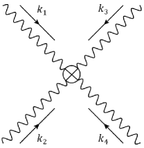
Figure 1: Dominant contribution to light-by-light scattering

The Feynman diagram for the tree-level process in Lorentz-violating QED is displayed in Fig. 1. The Feynman rule

$$-8i(k_{1})_{\mu_{1}}(k_{2})_{\mu_{2}}(k_{3})_{\mu_{3}}(k_{4})_{\mu_{4}}k_{F}^{(8)\mu_{1}\alpha_{1}\mu_{2}\alpha_{2}\mu_{3}\alpha_{3}\mu_{4}\alpha_{4}}$$ (34)

depends on the momenta of the four photon lines and is governed by the coefficient $k_{F}^{(8)\mu_{1}\alpha_{1}\mu_{2}\alpha_{2}\mu_{3}\alpha_{3}\mu_{4}\alpha_{4}}$. This coefficient is antisymmetric under the exchange of indices $\mu_{j}\leftrightarrow\alpha_{j}$ for each $j=1,2,3,4$. It is also totally symmetric under exchanges of any pair of indices $\mu_{j}\alpha_{j}$. These symmetries imply that the coefficient contains a total of 126 independent components, each describing a distinct physical effect.

The total cross section for light-by-light scattering is the integral of the spin-averaged squared modulus of the scattering amplitude over the phase space, as usual. In the laboratory frame, we denote the four-momenta of the two incoming photons by $k_{1}$ and $k_{2}$ and the four-momenta of the two outgoing photons by $k_{3}$ and $k_{4}$. The spin-averaged squared modulus of the scattering amplitude then takes the form

$$\hskip-5.0pt{\textstyle{\frac{1}{4}}}\Sigma\lvert\mathcal{T}_{fi}\rvert^{2}=16\eta_{\alpha_{1}\alpha_{1}^{\prime}}\eta_{\alpha_{2}\alpha_{2}^{\prime}}\eta_{\alpha_{3}\alpha_{3}^{\prime}}\eta_{\alpha_{4}\alpha_{4}^{\prime}}$$

$$\hskip 10.0pt\times(k_{1})_{\mu_{1}}(k_{1})_{\mu_{1}^{\prime}}(k_{2})_{\mu_{2}}(k_{2})_{\mu_{2}^{\prime}}(k_{3})_{\mu_{3}}(k_{3})_{\mu_{3}^{\prime}}(k_{4})_{\mu_{4}}(k_{4})_{\mu_{4}^{\prime}}$$

$$\hskip 10.0pt\times k_{F}^{(8)\mu_{1}\alpha_{1}\mu_{2}\alpha_{2}\mu_{3}\alpha_{3}\mu_{4}\alpha_{4}}k_{F}^{(8)\mu_{1}^{\prime}\alpha_{1}^{\prime}\mu_{2}^{\prime}\alpha_{2}^{\prime}\mu_{3}^{\prime}\alpha_{3}^{\prime}\mu_{4}^{\prime}\alpha_{4}^{\prime}}.$$ (35)

Note that this expression is quadratic in the coefficient $k_{F}^{(8)\mu_{1}\alpha_{1}\mu_{2}\alpha_{2}\mu_{3}\alpha_{3}\mu_{4}\alpha_{4}}$.

The result (35) exhibits an interesting duality symmetry. Direct calculation reveals that it is invariant under the replacement of $k_{F}^{(8)\mu_{1}\alpha_{1}\mu_{2}\alpha_{2}\mu_{3}\alpha_{3}\mu_{4}\alpha_{4}}$ with its quadruple dual $\widetilde{k}_{F}^{(8)\mu_{1}\alpha_{1}\mu_{2}\alpha_{2}\mu_{3}\alpha_{3}\mu_{4}\alpha_{4}}$ defined by

$$\hskip-20.0pt\widetilde{k}_{F}^{(8)\mu_{1}\alpha_{1}\mu_{2}\alpha_{2}\mu_{3}\alpha_{3}\mu_{4}\alpha_{4}}=\tfrac{1}{16}k^{(8)}_{F}{}_{\mu_{1}^{\prime}\alpha_{1}^{\prime}\mu_{2}^{\prime}\alpha_{2}^{\prime}\mu_{3}^{\prime}\alpha_{3}^{\prime}\mu_{4}^{\prime}\alpha_{4}^{\prime}}$$

$$\hskip 20.0pt\times\epsilon^{\mu_{1}\alpha_{1}\mu_{1}^{\prime}\alpha_{1}^{\prime}}\epsilon^{\mu_{2}\alpha_{2}\mu_{2}^{\prime}\alpha_{2}^{\prime}}\epsilon^{\mu_{3}\alpha_{3}\mu_{3}^{\prime}\alpha_{3}^{\prime}}\epsilon^{\mu_{4}\alpha_{4}\mu_{4}^{\prime}\alpha_{4}^{\prime}}.$$ (36)

This symmetry guarantees that the experimental constraints on a component of the coefficient and the corresponding component of its dual are the same.

Denoting by $\Omega$ the solid angle subtended by the momentum $\bf{k_{3}}$ relative to $\bf{k_{1}}$, the theoretical differential cross section $d\sigma/d\Omega$ can be written in the form

$$\frac{d\sigma}{d\Omega}=\frac{1}{256\pi^{2}[(\omega_{1}+\omega_{2})-(\omega_{1}-\omega_{2})\cos\theta]^{2}}\Sigma\lvert\mathcal{T}_{fi}\rvert^{2}.$$ (37)

In this expression, the energies of the two incoming photons are $\omega_{1}$ and $\omega_{2}$, and $\theta$ is the angle between the momenta $\bf{k_{1}}$ and $\bf{k_{3}}$. Note that the differential cross section has nontrivial dependence on the azimuthal scattering angle $\phi$ arising from the Lorentz violation in the scattering amplitude $\mathcal{T}_{fi}$.

IV.1.2 Cross section and constraints

Our present interest is the application of the above derivation to the data for light-by-light scattering obtained from ultraperipheral collisions of lead ions ma17 . The relevant process is shown schematically in Fig. 2, which displays the role of the four-point photon vertex. The photons from the high-energy lead ions can be viewed as photon beams in the equivalent photon approximation epa .

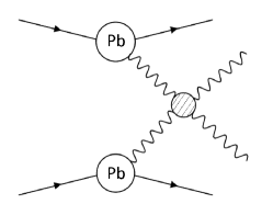
Figure 2: Light-by-light scattering in ultraperipheral collisions

In the experiment, the two incoming photons emitted by the lead ions are almost collinear. The experimental cross section can be taken as a convolution of the differential cross section (37) with the incoming photon-flux factors, integrated over the range of observed solid angle and outgoing photon energies es16 . It can be written in the form

$$\sigma^{\textrm{expt}}=\int d\Omega dm_{\gamma\gamma}dy_{\gamma\gamma}\frac{m_{\gamma\gamma}}{2}\frac{n(\omega_{1})}{\omega_{1}}\frac{n(\omega_{2})}{\omega_{2}}\frac{d\sigma}{d\Omega},$$ (38)

where the diphoton mass $m_{\gamma\gamma}=2\sqrt{\omega_{3}\omega_{4}}$ and the diphoton rapidity $y_{\gamma\gamma}=\ln(\omega_{4}/\omega_{3})/2$ are functions of the energies $\omega_{3}$ and $\omega_{4}$ of the outgoing photons. The photon-flux factors $n(\omega_{1})$ and $n(\omega_{2})$ depend on the incoming photon energies $\omega_{1}$, $\omega_{2}$, which can be expressed in terms of $\omega_{3}$, $\omega_{4}$ and the scattering angle $\theta$ by

$$\omega_{1} = {\textstyle{\frac{1}{2}}}\omega_{3}(1+\cos\theta)+{\textstyle{\frac{1}{2}}}\omega_{4}\left(1\pm\sqrt{1-\frac{\omega_{3}^{2}}{\omega_{4}^{2}}\sin^{2}\theta}\right),$$

$$\omega_{2} = {\textstyle{\frac{1}{2}}}\omega_{3}(1-\cos\theta)+{\textstyle{\frac{1}{2}}}\omega_{4}\left(1\mp\sqrt{1-\frac{\omega_{3}^{2}}{\omega_{4}^{2}}\sin^{2}\theta}\right).\qquad$$ (39)

For the calculation, we assume $\omega_{3}\leq\omega_{4}$ for convenience.

Table 7: Constraints from light-by-light scattering on the modulus of combinations of photon coefficients.

Limiting case	Coefficient combination	Constraint
Lorentz invariant	$\tfrac{1}{144}\eta_{\kappa\mu}\eta_{\lambda\nu}\eta_{\rho\tau}\eta_{\sigma\upsilon}k_{F}^{(8)\kappa\lambda\mu\nu\rho\sigma\tau\upsilon}$	$<9.5\times 10^{-8}\textrm{ GeV}^{-4}$
	$\tfrac{1}{576}\epsilon_{\kappa\lambda\mu\nu}\epsilon_{\rho\tau\sigma\upsilon}k_{F}^{(8)\kappa\lambda\mu\nu\rho\sigma\tau\upsilon}$	$<9.5\times 10^{-8}\textrm{ GeV}^{-4}$
	$\tfrac{1}{288}\eta_{\kappa\mu}\eta_{\lambda\nu}\epsilon_{\rho\tau\sigma\upsilon}k_{F}^{(8)\kappa\lambda\mu\nu\rho\sigma\tau\upsilon}$	$<7.5\times 10^{-8}\textrm{ GeV}^{-4}$
Isotropic	$\tfrac{1}{9}\sum_{J,K}k_{F}^{(8)TJTJTKTK}$	$<1.2\times 10^{-7}\textrm{ GeV}^{-4}$
	$\tfrac{1}{9}\sum_{J<K,L<M}k_{F}^{(8)JKJKLMLM}$	$<1.2\times 10^{-7}\textrm{ GeV}^{-4}$
	$\tfrac{1}{9}\sum_{J,M,K<L,N<P}\epsilon_{JKL}\epsilon_{MNP}k_{F}^{(8)TJTMKLNP}$	$<9.5\times 10^{-8}\textrm{ GeV}^{-4}$
	$\tfrac{1}{9}\sum_{J,K<L}k_{F}^{(8)TJTJKLKL}$	$<2.3\times 10^{-7}\textrm{ GeV}^{-4}$
	$\tfrac{1}{9}\sum_{J,K,L<M}\epsilon_{KLM}k_{F}^{(8)TJTJTKLM}$	$<5.6\times 10^{-8}\textrm{ GeV}^{-4}$
	$\tfrac{1}{9}\sum_{L,J<K,M<N}\epsilon_{LMN}k_{F}^{(8)JKJKTLMN}$	$<5.6\times 10^{-8}\textrm{ GeV}^{-4}$

The ATLAS experiment ma17 is sensitive to most of the $4\pi$ solid angle, implying that the integral (38) ranges over $0.18\mathrel{\hbox to0.0pt{\lower 4.0pt\hbox{\hskip 1.0pt$\sim$}\hss}\raise 1.0pt\hbox{$<$}}\theta\mathrel{\hbox to0.0pt{\lower 4.0pt\hbox{\hskip 1.0pt$\sim$}\hss}\raise 1.0pt\hbox{$<$}}2.96$ and $0\leq\phi\leq 2\pi$. The data span the diphoton-mass range 6 GeV$\mathrel{\hbox to0.0pt{\lower 4.0pt\hbox{\hskip 1.0pt$\sim$}\hss}\raise 1.0pt\hbox{$<$}}m_{\gamma\gamma}\mathrel{\hbox to0.0pt{\lower 4.0pt\hbox{\hskip 1.0pt$\sim$}\hss}\raise 1.0pt\hbox{$<$}}$ 24 GeV, so we restrict the integral (38) to this range and adopt the corresponding diphoton-rapidity range $0\mathrel{\hbox to0.0pt{\lower 4.0pt\hbox{\hskip 1.0pt$\sim$}\hss}\raise 1.0pt\hbox{$<$}}y_{\gamma\gamma}\mathrel{\hbox to0.0pt{\lower 4.0pt\hbox{\hskip 1.0pt$\sim$}\hss}\raise 1.0pt\hbox{$<$}}\ln(m_{\gamma\gamma}/6)$. Unlike the SM result, which is tiny for large diphoton masses, the maximum of $\sigma^{\textrm{expt}}$ in Lorentz-violating QED is attained for a diphoton mass of around 600 GeV. Our restriction on the upper value of the diphoton mass therefore ultimately translates into conservative constraints on the coefficients $k_{F}^{(8)\mu_{1}\alpha_{1}\mu_{2}\alpha_{2}\mu_{3}\alpha_{3}\mu_{4}\alpha_{4}}$. Future experiments at higher energies can be expected to increase significantly the sensitivity to these effects.

The photon-flux function $n(\omega)$ is determined by the elastic form factor $F(q^{2})$, which is the Fourier transformation of the charge distribution of the nucleus. It can be written as gb02

$$n(\omega)=\frac{Z^{2}\alpha}{\pi^{2}}\int d^{2}q_{\perp}\frac{q_{\perp}^{2}}{\big{[}(\omega/\gamma)^{2}+q_{\perp}^{2}\big{]}^{2}}F^{2}\left(\left[\frac{\omega}{\gamma}\right]^{2}+q_{\perp}^{2}\right),$$ (40)

where $Z$ is the atomic number of the ion, $\alpha\simeq/137$ is the fine-structure constant, $\gamma=1/\sqrt{1-\beta^{2}}$ is the Lorentz factor of the nucleus, $q_{\perp}$ is the transverse momentum, and the integral of $q_{\perp}$ ranges over the whole plane. Taking the form factor as gb02 $F(q^{2})=\Theta(1/R^{2}-q^{2})$, where $R$ is the nuclear radius, yields $n(\omega)=({2Z^{2}\alpha}/{\pi})\ln({\gamma}/{\omega R})$ at leading order. However, this expression for the photon flux becomes negative for $\omega>\gamma/R$, which is potentially problematic. Instead, we approximate $F(q^{2})$ as a monopole form factor htb94 $F(q^{2})={\Lambda^{2}}/({\Lambda^{2}+q^{2}})$, where $\Lambda=\sqrt{6/\langle r^{2}\rangle}$ and $\langle r^{2}\rangle$ is mean squared radius of the nucleus. For ${}^{208}\textrm{Pb}$, experimental data vjv87 give $\langle r^{2}\rangle^{1/2}=5.5$ fm and $\Lambda=0.088$ GeV. We find that the photon-flux function (40) then becomes

$$n(\omega)=\frac{2Z^{2}\alpha}{\pi}\left[\frac{2(\omega/\gamma)^{2}+\Lambda^{2}}{2\Lambda^{2}}\ln\Big{(}1+\frac{\Lambda^{2}}{(\omega/\gamma)^{2}}\Big{)}-1\right].$$ (41)

This expression is positive for any $\omega$ and converges to zero as $\omega$ tends to infinity, matching physical expectations. For definiteness and simplicity, we use the above expression to calculate the cross section. As a cross check, we have also used the fivefold integral presented in the literature ks10 to estimate the photon flux and calculate the cross section, obtaining results close to those using the expression (41).

The LHC experiment measured the cross section as 70$\pm$24(stat.)$\pm$17(syst.) nb ma17 . The theoretical SM prediction is 49$\pm$10 nb ks10 . The difference between these results is 21$\pm$31 nb, which is compatible with zero. An upper limit for the additional tree-level contribution in Lorentz-violating QED can therefore be taken as 83 nb at the 95% confidence level. We can use this result to constrain the coefficients $k_{F}^{(8)\mu_{1}\alpha_{1}\mu_{2}\alpha_{2}\mu_{3}\alpha_{3}\mu_{4}\alpha_{4}}$.

The rotation of the Earth and its revolution about the Sun imply that the laboratory is a noninertial frame, which induces time dependence in the coefficients for Lorentz violation. Experimental results on the coefficients must therefore be reported in a prescribed inertial frame. By standard convention in the literature, this frame is taken to be the Sun-centered frame sunframe with spatial coordinates $X^{J}$, $J=X,Y,Z$ chosen so that the $Z$ axis is aligned along the rotation axis of the Earth. The $X$ axis points from the Earth to the Sun at the 2000 vernal equinox, which is adopted as the origin of the time $T$. The $Y$ axis completes the right-handed orthogonal coordinate system. The contribution to the cross section therefore can be viewed as determined by a nonlinear combination of the 126 independent components of the coefficient $k_{F}^{(8)\mu_{1}\alpha_{1}\mu_{2}\alpha_{2}\mu_{3}\alpha_{3}\mu_{4}\alpha_{4}}$ expressed in the Sun-centered frame. The experimental result from the LHC places a single constraint on this combination. However, the result is unwieldy. To gain insight, we follow here the standard practice in the literature of extracting constraints in various limiting scenarios.

Table 8: Constraints from light-by-light scattering on the modulus of individual photon coefficients.

Coefficient	Constraint
$k_{F}^{(8)TXTXTXTX},k_{F}^{(8)TYTYTYTY},k_{F}^{(8)XZXZXZXZ},k_{F}^{(8)YZYZYZYZ}$	$<1.0\times 10^{-6}\textrm{ GeV}^{-4}$
$k_{F}^{(8)TZTZTZTZ},k_{F}^{(8)XYXYXYXY}$	$<5.9\times 10^{-7}\textrm{ GeV}^{-4}$
$k_{F}^{(8)TXTXTXTY},k_{F}^{(8)TYTYTYTX},k_{F}^{(8)XZXZXZYZ},k_{F}^{(8)YZYZYZXZ}$	$<6.4\times 10^{-7}\textrm{ GeV}^{-4}$
$k_{F}^{(8)TXTXTXTZ},k_{F}^{(8)TYTYTYTZ},k_{F}^{(8)XZXZXZXY},k_{F}^{(8)YZYZYZXY}$	$<4.9\times 10^{-7}\textrm{ GeV}^{-4}$
$k_{F}^{(8)TXTXTXXY},k_{F}^{(8)TYTYTYXY},k_{F}^{(8)XZXZXZTZ},k_{F}^{(8)YZYZYZTZ}$	$<5.5\times 10^{-7}\textrm{ GeV}^{-4}$
$k_{F}^{(8)TXTXTXXZ},k_{F}^{(8)TYTYTYYZ},k_{F}^{(8)XZXZXZTX},k_{F}^{(8)YZYZYZTY}$	$<1.0\times 10^{-6}\textrm{ GeV}^{-4}$
$k_{F}^{(8)TXTXTXYZ},k_{F}^{(8)TYTYTYXZ},k_{F}^{(8)XZXZXZTY},k_{F}^{(8)YZYZYZTX}$	$<5.2\times 10^{-7}\textrm{ GeV}^{-4}$
$k_{F}^{(8)TZTZTZTX},k_{F}^{(8)TZTZTZTY},k_{F}^{(8)XYXYXYXZ},k_{F}^{(8)XYXYXYYZ}$	$<3.8\times 10^{-7}\textrm{ GeV}^{-4}$
$k_{F}^{(8)TZTZTZXY},k_{F}^{(8)XYXYXYTZ}$	$<3.0\times 10^{-7}\textrm{ GeV}^{-4}$
$k_{F}^{(8)TZTZTZXZ},k_{F}^{(8)TZTZTZYZ},k_{F}^{(8)XYXYXYTX},k_{F}^{(8)XYXYXYTY}$	$<4.2\times 10^{-7}\textrm{ GeV}^{-4}$
$k_{F}^{(8)TXTXTYTY},k_{F}^{(8)XZXZYZYZ}$	$<5.6\times 10^{-7}\textrm{ GeV}^{-4}$
$k_{F}^{(8)TXTXTZTZ},k_{F}^{(8)TYTYTZTZ},k_{F}^{(8)XYXYXZXZ},k_{F}^{(8)XYXYYZYZ}$	$<3.6\times 10^{-7}\textrm{ GeV}^{-4}$
$k_{F}^{(8)TXTXXYXY},k_{F}^{(8)TYTYXYXY},k_{F}^{(8)TZTZXZXZ},k_{F}^{(8)TZTZYZYZ}$	$<9.7\times 10^{-7}\textrm{ GeV}^{-4}$
$k_{F}^{(8)TXTXXZXZ},k_{F}^{(8)TYTYYZYZ}$	$<1.1\times 10^{-6}\textrm{ GeV}^{-4}$
$k_{F}^{(8)TXTXYZYZ},k_{F}^{(8)TYTYXZXZ}$	$<4.3\times 10^{-7}\textrm{ GeV}^{-4}$
$k_{F}^{(8)TZTZXYXY}$	$<2.4\times 10^{-7}\textrm{ GeV}^{-4}$
$k_{F}^{(8)TXTXTYTZ},k_{F}^{(8)TYTYTXTZ},k_{F}^{(8)XZXZXYYZ},k_{F}^{(8)YZYZXYXZ}$	$<3.4\times 10^{-7}\textrm{ GeV}^{-4}$
$k_{F}^{(8)TXTXTYXY},k_{F}^{(8)TYTYTXXY},k_{F}^{(8)XZXZTZYZ},k_{F}^{(8)YZYZTZXZ}$	$<4.0\times 10^{-7}\textrm{ GeV}^{-4}$
$k_{F}^{(8)TXTXTYXZ},k_{F}^{(8)TYTYTXYZ},k_{F}^{(8)XZXZTXYZ},k_{F}^{(8)YZYZTYXZ}$	$<5.2\times 10^{-7}\textrm{ GeV}^{-4}$
$k_{F}^{(8)TXTXTYYZ},k_{F}^{(8)TYTYTXXZ},k_{F}^{(8)XZXZTYYZ},k_{F}^{(8)YZYZTXXZ}$	$<4.2\times 10^{-7}\textrm{ GeV}^{-4}$
$k_{F}^{(8)TXTXTZXY},k_{F}^{(8)TYTYTZXY},k_{F}^{(8)YZYZTZXY},k_{F}^{(8)XZXZTZXY}$	$<2.8\times 10^{-7}\textrm{ GeV}^{-4}$
$k_{F}^{(8)TZTZTXYZ},k_{F}^{(8)TZTZTYXZ},k_{F}^{(8)XYXYTXYZ},k_{F}^{(8)XYXYTYXZ}$	$<2.8\times 10^{-7}\textrm{ GeV}^{-4}$
$k_{F}^{(8)TXTXTZXZ},k_{F}^{(8)TYTYTZYZ},k_{F}^{(8)XZXZTXXY},k_{F}^{(8)YZYZTYXY}$	$<5.1\times 10^{-7}\textrm{ GeV}^{-4}$
$k_{F}^{(8)TXTXTZYZ},k_{F}^{(8)TYTYTZXZ},k_{F}^{(8)XZXZTYXY},k_{F}^{(8)YZYZTXXY}$	$<2.9\times 10^{-7}\textrm{ GeV}^{-4}$
$k_{F}^{(8)TXTXXYXZ},k_{F}^{(8)TYTYXYYZ},k_{F}^{(8)XZXZTXTZ},k_{F}^{(8)YZYZTYTZ}$	$<6.0\times 10^{-7}\textrm{ GeV}^{-4}$
$k_{F}^{(8)TXTXXYYZ},k_{F}^{(8)TYTYXYXZ},k_{F}^{(8)XZXZTYTZ},k_{F}^{(8)YZYZTXTZ}$	$<3.0\times 10^{-7}\textrm{ GeV}^{-4}$
$k_{F}^{(8)TXTXXZYZ},k_{F}^{(8)TYTYXZYZ},k_{F}^{(8)XZXZTXTY},k_{F}^{(8)YZYZTXTY}$	$<4.8\times 10^{-7}\textrm{ GeV}^{-4}$
$k_{F}^{(8)TZTZTXTY},k_{F}^{(8)XYXYXZYZ}$	$<2.9\times 10^{-7}\textrm{ GeV}^{-4}$
$k_{F}^{(8)TZTZTXXY},k_{F}^{(8)TZTZTYXY},k_{F}^{(8)XYXYTZXZ},k_{F}^{(8)XYXYTZYZ}$	$<2.3\times 10^{-7}\textrm{ GeV}^{-4}$
$k_{F}^{(8)TZTZTXXZ},k_{F}^{(8)TZTZTYYZ},k_{F}^{(8)XYXYTXXZ},k_{F}^{(8)XYXYTYYZ}$	$<3.9\times 10^{-7}\textrm{ GeV}^{-4}$
$k_{F}^{(8)TZTZXYXZ},k_{F}^{(8)TZTZXYYZ},k_{F}^{(8)XYXYTXTZ},k_{F}^{(8)XYXYTYTZ}$	$<2.4\times 10^{-7}\textrm{ GeV}^{-4}$
$k_{F}^{(8)TZTZXZYZ},k_{F}^{(8)XYXYTXTY}$	$<7.3\times 10^{-7}\textrm{ GeV}^{-4}$
$k_{F}^{(8)TXTYTZXY},k_{F}^{(8)TZXYXZYZ}$	$<2.2\times 10^{-7}\textrm{ GeV}^{-4}$
$k_{F}^{(8)TXTYTZXZ},k_{F}^{(8)TXTYTZYZ},k_{F}^{(8)TXXYXZYZ},k_{F}^{(8)TYXYXZYZ}$	$<2.9\times 10^{-7}\textrm{ GeV}^{-4}$
$k_{F}^{(8)TXTYXYXZ},k_{F}^{(8)TXTYXYYZ},k_{F}^{(8)TXTZXZYZ},k_{F}^{(8)TYTZXZYZ}$	$<3.2\times 10^{-7}\textrm{ GeV}^{-4}$
$k_{F}^{(8)TXTYXZYZ}$	$<3.4\times 10^{-7}\textrm{ GeV}^{-4}$
$k_{F}^{(8)TXTZXYXZ},k_{F}^{(8)TYTZXYYZ}$	$<3.8\times 10^{-7}\textrm{ GeV}^{-4}$
$k_{F}^{(8)TXTZXYYZ},k_{F}^{(8)TYTZXYXZ}$	$<3.5\times 10^{-7}\textrm{ GeV}^{-4}$

Consider first the Lorentz-invariant limit. Inspection of Table 5 reveals that there are three Lorentz-invariant combinations of components of the coefficient $k_{F}^{(8)\mu_{1}\alpha_{1}\mu_{2}\alpha_{2}\mu_{3}\alpha_{3}\mu_{4}\alpha_{4}}$. The orientation and velocity of the laboratory relative to the canonical Sun-centered frame plays no role for these combinations, so constraints can be derived directly from the experimental data. The first three rows of Table 7 lists the results of this analysis. Each row specifies a Lorentz-invariant coefficient combination and the corresponding constraint, obtained under the assumption that other independent coefficient combinations vanish. The fractions appearing in front of the combinations are chosen to insure the combination has the same weight as a single component of $k_{F}^{(8)\mu_{1}\alpha_{1}\mu_{2}\alpha_{2}\mu_{3}\alpha_{3}\mu_{4}\alpha_{4}}$. In terms of the invariants (30), the operators in the Lagrange density associated with the first, second, and third row are $X^{2}$, $Y^{2}$, and $XY$, respectively.

We can also consider the isotropic limit of Lorentz-violating QED. According to the results in Table 6, the coefficient $k_{F}^{(8)\mu_{1}\alpha_{1}\mu_{2}\alpha_{2}\mu_{3}\alpha_{3}\mu_{4}\alpha_{4}}$ contains six isotropic combinations of components. Since isotropic effects are independent of the laboratory orientation and since the laboratory boost $\beta\simeq 10^{-4}$ is negligible in the Sun-centered frame, we can again obtain constraints on the isotropic combinations directly from an analysis performed in the laboratory. The resulting constraints in the Sun-centered frame are displayed in the second part of Table 7. The isotropic combinations are listed in the second column, where the summations are over spatial indices $J$, $K$, $\ldots=X,Y,Z$. The third column presents the corresponding constraint on the modulus of each combination expressed in the Sun-centered frame, determined assuming other coefficient components vanish. The constraints on the first two and last two isotropic combinations are identical, as a consequence of the duality symmetry associated with the quadruply dualized coefficients (36).

To implement a complete analysis, the cross section expressed using coefficients in the laboratory frame must be transformed to the Sun-centered frame. To a good approximation, the small Earth boost can be neglected in the transformation. Denoting the spatial coordinates in the laboratory frame by $x^{j}$, the rotation matrix between the two frames is given by

$$R^{jJ}=\left(\begin{array}[]{ccc}\cos\chi\cos\omega_{\oplus}T_{\oplus}&\cos\chi\sin\omega_{\oplus}T_{\oplus}&-\sin\chi\\ -\sin\omega_{\oplus}T_{\oplus}&\cos\omega_{\oplus}T_{\oplus}&0\\ \sin\chi\cos\omega_{\oplus}T_{\oplus}&\sin\chi\sin\omega_{\oplus}T_{\oplus}&\cos\chi\end{array}\right),$$ (42)

where $\omega_{\oplus}\simeq 2\pi/(23{\rm~{}h}~{}56{\rm~{}min})$ is the Earth’s sidereal rotation frequency, $T_{\oplus}$ is a convenient local sidereal time, and $\chi$ is the angle between the beam direction and the $Z$ axis. For the ATLAS detector at the LHC, $\chi\simeq 81.4^{\circ}$.

Implementing this transformation on the cross section generates a lengthy expression containing up to fourth harmonics of the sidereal frequency. The measured cross section is therefore predicted to display sidereal variations in time at all these harmonics. Analyzing experimental data to search for these time variations would be of great interest, but insufficient data are presently available to implement this. Instead, we consider here the time-averaged cross section, which selects the time-independent contributions for consideration. Calculation reveals that all 126 independent components of $k_{F}^{(8)\mu_{1}\alpha_{1}\mu_{2}\alpha_{2}\mu_{3}\alpha_{3}\mu_{4}\alpha_{4}}$ contribute to this result.

Table 8 presents the constraints on all 126 components, taken one at a time with all others set to zero. The first column lists the components, and the second column shows the constraint on the modulus of each one. These results are the first in the literature on nonlinear Lorentz-violating photon interactions. Existing constraints on $d=8$ pure-photon terms in Lorentz-violating QED are restricted to effects on photon propagation in the astrophysical and laboratory contexts km ; d8astro ; d8lab . Inspection confirms that the constraints in the table exhibit the duality symmetry associated with Eq. (36), as expected. The results also reveal symmetry under interchange of the $X$ and $Y$ indices. This is a consequence of the rotation of the Earth about the $Z$ axis, which implies that the time-averaged cross section must be invariant under rotation in the $X$-$Y$ plane and hence under the exchange $(X,Y)\leftrightarrow(Y,-X)$. The sign in this exchange has no effect on the constraints because the cross section depends only on the square of the coefficients.

IV.2 Deep inelastic scattering

Deep inelastic scattering offers crucial experimental support for the existence of quarks and the predictions of QCD, and it serves as a tool in searches for physics beyond the SM dis ; disproc . An initial study of the effects of Lorentz violation on deep inelastic electron-proton scattering klv17 has studied the use of DIS to search for Lorentz-violating effects of $c$-type coefficients in the QCD and QED interactions of quarks. This work complements recent theoretical and experimental efforts to investigate Lorentz and CPT violation in the quark sector involving operators of mass dimensions $d=3$ ak98 ; d3quark , $d=4$ d4quark , and $d=5$ nvt16 . The construction of the nonminimal operators given in Table 4 offers numerous interesting prospects for further exploration in Lorentz-violating QCD.

Here, we illustrate the possibilities by investigating the effects on the DIS cross section of a subset of nonminimal Lorentz- and CPT-violating terms in the Lagrange density for QCD and QED coupled to quarks. Following the general approach presented in Ref. klv17 , we focus on unpolarized electron-proton DIS, for which it suffices to limit attention to spin-independent operators. For definiteness, we work with spin-independent operators of lowest nonminimal mass dimension, which turn out to be governed by the $a^{(5)}$- and $a_{F}^{(5)}$-type coefficients. Calculation reveals that the $a_{F}^{(5)}$-type coefficients leave unaffected the DIS cross section at leading order, so in what follows we focus on the experimentally measurable signals produced by the $a^{(5)}$-type coefficients.

IV.2.1 Setup

For electron-proton DIS, the relevant terms in the Lagrange density that involve the valence quarks in the proton are

$$\hskip-25.0pt-{\textstyle{\frac{1}{2}}}\sum_{f}a_{f}^{(5)\mu\alpha\beta}\overline{\psi}{}_{f}\gamma_{\mu}iD_{(\alpha}iD_{\beta)}\psi_{f}+\textrm{h.c.}$$ (43)

$$= -\sum_{f}a_{f}^{(5)\mu\alpha\beta}\big{[}\overline{\psi}{}_{f}\gamma_{\mu}i\partial_{\alpha}i\partial_{\beta}\psi_{f}-q_{f}A_{\alpha}\overline{\psi}{}_{f}\gamma_{\mu}i\partial_{\beta}\psi_{f}$$

$$\hskip 25.0pt+q_{f}A_{\alpha}(i\partial_{\beta}\overline{\psi}{}_{f})\gamma_{\mu}\psi_{f}+q_{f}^{2}A_{\alpha}A_{\beta}\overline{\psi}{}_{f}\gamma_{\mu}\psi_{f}\big{]},$$

where some surface terms are neglected. In this expression, we limit attention to flavor-diagonal effects and the two dominant quark flavors $f=u$, $d$. The coefficients $a^{(5)\mu\alpha\beta}_{f}$ are symmetric under interchange of the last two indices, $a^{(5)\mu\alpha\beta}_{f}=a^{(5)\mu\beta\alpha}_{f}$.

At leading order, the DIS process of interest involves the exchange of a photon between the scattered electron and the proton. We can therefore in principle expect Lorentz-violating effects in the photon and electron sectors to play a role, along with potential effects caused by the binding of the valence quarks to form the proton. For simplicity and definiteness, we neglect here effects from the photon and electron sectors, many of which are already tightly bounded tables . Note in particular that existing limits on $d=5$ operators in the photon sector lie far below DIS sensitivities km ; photon . Also, while precision studies of $d=5$ operators in the electron sector are less broadly constrained km ; ms16 ; kv18 , they nonetheless also lie below the DIS sensitivities estimated below. In contrast, in the $d=5$ proton sector the coefficients $a^{(5)\mu\alpha\beta}_{p}$ are only partially bounded kv18 , and the existing DIS sensitivities are roughly comparable to those estimated below. Since the structure of the proton is nontrivial and little is known about Lorentz and CPT violation in the strong binding by the gluons and sea species, we treat the coefficients $a^{(5)\mu\alpha\beta}_{f}$ and $a^{(5)\mu\alpha\beta}_{p}$ as independent here.

Coefficients of the $a^{(5)}$ type affect various particle properties. Consider first effects at the level of relativistic quantum mechanics. In the presence of these Lorentz- and CPT-violating effects, the Dirac equation for a freely propagating fermion is modified to

$$(i\gamma_{\mu}\partial^{\mu}-a^{(5)\mu\alpha\beta}\gamma_{\mu}i\partial_{\alpha}i\partial_{\beta}-m)\psi=0.$$ (44)

For perturbative Lorentz violation, this equation has two positive-energy and two negative-energy solutions. As usual, we reinterpret the negative-energy solutions as positive-energy antiparticle solutions with reversed momentum. The plane-wave eigenfunctions can be written as $\psi^{(s)}(x)=\exp(-ip_{u}\cdot x)u^{(s)}({\bf p},a)$ for the positive-energy solutions and $\psi^{(s)}(x)=\exp(+ip_{v}\cdot x)v^{(s)}({\bf p},a)$ for the negative-energy ones, where $p_{u}^{\mu}=(E_{u},\bf{p})$ and $p_{v}^{\mu}=(E_{v},\bf{p})$ are the four-momenta of the particle and antiparticle, $\bf{p}$ is the three momentum, and $s=1,2$ labels the spin.

Since the Lorentz-violating terms in the Lagrange density contain only spin-independent operators, the energies $E_{u}$ and $E_{v}$ are independent of the spins. However, the Lorentz violation typically implies that $E_{u}\neq E_{v}$, as can be seen from the dispersion relations

$$(p_{u}^{\mu}-a^{(5)\mu p_{u}p_{u}})\eta_{\mu\nu}(p_{u}^{\nu}-a^{(5)\nu p_{u}p_{u}}) = m^{2},$$

$$(p_{v}^{\mu}+a^{(5)\mu p_{v}p_{v}})\eta_{\mu\nu}(p_{v}^{\nu}+a^{(5)\nu p_{v}p_{v}}) = m^{2}.$$ (45)

In these expressions, an index $p_{u}$ or $p_{v}$ implies contraction with the corresponding four-momentum. For example, we write $a^{(5)\mu p_{u}p_{u}}\equiv a^{(5)\mu\alpha\beta}p_{u\alpha}p_{u\beta}$. The dispersion relations (45) reveal that the energies of the particle and antiparticle are related by $E_{u}({\bf p},a)=E_{v}({\bf p},-a)$, as is expected given that the $a^{(5)}$-type coefficients govern CPT-odd operators.

The momentum-space solutions of the modified Dirac equation (44) can be written as

$$u^{(s)}({\bf p},a) = \frac{p_{u}^{\mu}\gamma_{\mu}-a^{(5)\mu p_{u}p_{u}}\gamma_{\mu}+m}{\sqrt{E_{u}-a^{(5)0p_{u}p_{u}}+m}}u^{(s)}_{0},$$

$$v^{(s)}({\bf p},a) = \frac{-p_{v}^{\mu}\gamma_{\mu}-a^{(5)\mu p_{v}p_{v}}\gamma_{\mu}+m}{\sqrt{E_{v}+a^{(5)0p_{v}p_{v}}+m}}v^{(s)}_{0},$$ (46)

where $u^{(1)}_{0}{}^{\dagger}=(1,0,0,0)$, $u^{(2)}_{0}{}^{\dagger}=(0,1,0,0)$ and similarly $v^{(1)}_{0}{}^{\dagger}=(0,0,1,0)$, $v^{(2)}_{0}{}^{\dagger}=(0,0,0,1)$. These solutions can be obtained from the conventional Lorentz-invariant ones by the substitutions $p^{\mu}\to p_{u}^{\mu}-a^{(5)\mu p_{u}p_{u}}$ and $p^{\mu}\to p_{v}^{\mu}+a^{(5)\mu p_{v}p_{v}}$. They therefore obey the usual normalization relations,

$$\overline{u}^{(s)}({\bf p},a)u^{(s^{\prime})}({\bf p},a)=-\overline{v}^{(s)}({\bf p},a)v^{(s^{\prime})}({\bf p},a)=2m\delta^{ss^{\prime}}.$$ (47)

However, the traditional orthogonality relations are replaced by

$$\overline{u}^{(s)}({\bf p},a)v^{(s^{\prime})}({\bf p},-a)=\overline{v}^{(s)}({\bf p},a)u^{(s^{\prime})}({\bf p},-a)=0,$$ (48)

incorporating a sign change of the coefficients.

The solutions (46) imply modifications to the conventional spin sums. We find

$$\sum_{s}u^{(s)}({\bf p},a)\overline{u}^{(s)}({\bf p},a) = p_{u}^{\alpha}\gamma_{\alpha}-a^{(5)\alpha p_{u}p_{u}}\gamma_{\alpha}+m,$$

$$\sum_{s}v^{(s)}({\bf p},a)\overline{v}^{(s)}({\bf p},a) = p_{v}^{\alpha}\gamma_{\alpha}+a^{(5)\alpha p_{v}p_{v}}\gamma_{\alpha}-m.\qquad$$ (49)

As in the usual Lorentz-invariant case, we can write two projection operators from these expressions,

$$\Lambda_{u}({\bf p},a) = \frac{1}{2m}\sum_{s}u^{(s)}({\bf p},a)\overline{u}^{(s)}({\bf p},a),$$

$$\Lambda_{v}({\bf p},a) = -\frac{1}{2m}\sum_{s}v^{(s)}({\bf p},a)\overline{v}^{(s)}({\bf p},a).$$ (50)

As required, both these operators are idempotent, $\Lambda_{u}({\bf p},a)^{2}=\Lambda_{u}({\bf p},a)$ and $\Lambda_{v}({\bf p},a)^{2}=\Lambda_{v}({\bf p},a)$, and hence can be used as projectors in the two energy subspaces. However, they are no longer directly complementary. Instead, we find $\Lambda_{u}({\bf p},a)+\Lambda_{v}({\bf p},-a)=1$.

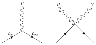
Figure 3: The $A\psi\psi$ vertex (left) and the $AA\psi\psi$ vertex (right).

At the level of the quantum field theory, the modified Feynman propagator is found to be

$$iS_{F}(p)=\frac{i}{\gamma_{\mu}p^{\mu}-a^{(5)\mu\alpha\beta}\gamma_{\mu}p_{\alpha}p_{\beta}-m+i\epsilon}.$$ (51)

The Feynman rule for the photon-fermion-fermion vertex shown in Fig. 3 becomes

$$-iq\Gamma^{\mu}(p_{\textrm{in}},p_{\textrm{out}})=-iq[\gamma^{\mu}-a^{(5)\alpha\beta\mu}\gamma_{\alpha}(p_{\textrm{in}}+p_{\textrm{out}})_{\beta}],$$ (52)

where $p_{\textrm{in}}$ and $p_{\textrm{out}}$ are the four-momenta of the incoming and outgoing fermions. The coefficient $a^{(5)}{}^{\alpha\beta\mu}$ is also associatd with a new vertex involving two photon lines and two fermion lines, as displayed in Fig. 3. The corresponding Feynman rule is

$$iq^{2}\Gamma^{(4)\mu\nu}=-2iq^{2}a^{(5)\alpha\mu\nu}\gamma_{\alpha}.$$ (53)

This vertex does not contribute to the DIS process at tree level, but it must be included if loops are considered.

IV.2.2 Cross section and constraints

The DIS differential cross section is a function of the phase-space variables for the scattered electron. Taking the $z$ axis as aligned with the incoming beam direction and denoting by $\theta$, $\phi$ the scattering angles of the electron in spherical polar coordinates, the four-momenta for the incoming electron, incoming proton, and outgoing electron can be written as $k^{\mu}=E(1,0,0,1)$, $p^{\mu}=E_{p}(1,0,0,-1)$, and $k^{\prime\mu}=E^{\prime}(1,\sin\theta\cos\phi,\sin\theta\sin\phi,\cos\theta)$, respectively. The intermediate photon then has four-momentum $q=k-k^{\prime}$. It is convenient to introduce the standard Mandelstam $s$ and Bjorken $x$ and $y$ variables via

$$s=(p+k)^{2},\quad x=\frac{-q^{2}}{2p\cdot q},\quad y=\frac{p\cdot q}{p\cdot k}.$$ (54)

In the expressions to follow, we can safely disregard the proton mass $M$ because in DIS experiments $M^{2}\ll Q^{2}=-q^{2}$ and $M^{2}\ll 2p\cdot q$. The quark masses can similarly be neglected.

In the presence of Lorentz violation, the unpolarized differential cross section for the DIS process can be written in the form klv17

$$\frac{d\sigma}{dxdyd\phi}=\frac{\alpha^{2}y}{2\pi q^{4}}L_{\mu\nu}\hbox{Im}\,W^{\mu\nu},$$ (55)

where $\alpha$ is the fine structure constant, $L_{\mu\nu}=2(k_{\mu}k^{\prime}_{\nu}+k_{\nu}k^{\prime}_{\mu}-k\cdot k^{\prime}\eta_{\mu\nu})$ is the electron tensor, and $W^{\mu\nu}$ is the proton tensor. To calculate the explicit form of $W^{\mu\nu}$, we use the parton model. Since the coefficients $a^{(5)\mu\alpha\beta}$ are assumed perturbatively small, we keep only terms at first order in what follows.

In the standard parton model, the parton momentum $p_{f}=\xi p$ is taken to be a fraction $\xi$ of the proton momentum $p$. However, the modified dispersion relation (45) enforces the conditions $p^{2}=2a_{p}^{(5)}{}^{ppp}$ and $p_{f}^{2}=2a_{f}^{(5)}{}^{p_{f}p_{f}p_{f}}$, which are incompatible with $p_{f}=\xi p$. Instead, we assume $p_{f}^{\mu}=\xi p^{\mu}+\delta_{f}^{\mu}$ with a small momentum correction $\delta_{f}^{\mu}$. Noting that $p\cdot\delta_{f}=\xi^{2}a_{f}^{(5)}{}{ppp}-\xi a_{p}^{(5)}{}^{ppp}$, we find

$$p_{f}^{\mu}=\xi p^{\mu}-\xi a_{p}^{(5)\mu pp}+\xi^{2}a_{f}^{(5)\mu pp}.$$ (56)

The implication of this shift for the parton distribution functions is an interesting topic for future investigation.

Following the treatment in Ref. klv17 , we can use the parton model and the optical theorem to obtain the explicit form of $\hbox{Im}\,W^{\mu\nu}$. The contribution involving the $AA\psi\psi$ vertex shown in Fig. 3 is purely real and so is irrelevant in this context. After some calculation, we find that the contribution involving the $A\psi\psi$ vertex is

$$W^{\mu\nu} = -{\textstyle{\frac{1}{2}}}\int_{0}^{1}d\xi\sum_{f}q_{f}^{2}\frac{f_{f}(\xi)}{\xi}$$ (57)

$$\hskip-30.0pt\times\textrm{tr}\Big{[}\gamma_{\alpha}(p_{f}^{\alpha}-a_{f}^{(5)\alpha p_{f}p_{f}})\big{(}\gamma^{\mu}-a_{f}^{(5)\alpha^{\prime}\beta^{\prime}\mu}\gamma_{\alpha^{\prime}}(2p_{f}+q)_{\beta^{\prime}}\big{)}$$

$$\times\gamma_{\beta}\big{(}p_{f}^{\beta}+q^{\beta}-a_{f}^{(5)\beta\rho\sigma}(p_{f}+q)_{\rho}(p_{f}+q)_{\sigma}\big{)}$$

$$\times\big{(}\gamma^{\nu}-a_{f}^{(5)\alpha^{\prime\prime}\beta^{\prime\prime}\nu}\gamma_{\alpha^{\prime\prime}}(2p_{f}+q)_{\beta^{\prime\prime}}\big{)}\Big{]}$$

$$\hskip-30.0pt\times\Big{(}\big{[}\gamma_{\beta}\big{(}p_{f}^{\beta}+q^{\beta}-a_{f}^{(5)\beta\rho\sigma}(p_{f}+q)_{\rho}(p_{f}+q)_{\sigma}\big{)}\big{]}^{2}+i\epsilon\Big{)}^{-1}$$

$$+(\mu\leftrightarrow\nu,q\leftrightarrow-q),$$

We are interested in the imaginary part of this expression. This comes from the propagator factor,

$$\textrm{Im}\big{(}\big{[}\gamma_{\beta}\big{(}p_{f}^{\beta}+q^{\beta}-a_{f}^{(5)\beta\rho\sigma}(p_{f}+q)_{\rho}(p_{f}+q)_{\sigma}\big{)}\big{]}^{2}+i\epsilon\big{)}^{-1}$$

$$\hskip 20.0pt=-\delta_{f}\delta(\xi-x^{\prime}_{f}),$$ (58)

where

$$\delta_{f} = \frac{\pi}{ys}\bigg{[}1+\frac{2}{s}a_{p}^{(5)}{}^{ppp}$$

$$+\frac{2}{ys}(a_{p}^{(5)}{}^{qpp}+4xa_{f}^{(5)}{}^{ppq}+2a_{f}^{(5)}{}^{qqp}+a_{f}^{(5)}{}^{pqq})\bigg{]},$$

and $x^{\prime}_{f}=x-x_{f}$ with

$$x_{f} = -\frac{2}{ys}(xa_{p}^{(5)}{}^{qpp}+2x^{2}a_{f}^{(5)}{}^{ppq}$$ (60)

$$\hskip 30.0pt+2xa_{f}^{(5)}{}^{qqp}+xa_{f}^{(5)}{}^{pqq}+a_{f}^{(5)}{}^{qqq}).$$

As a check on these calculations, we have used the explicit results for $\delta_{f}$ and $x_{f}$ to verify the Ward identity $q_{\mu}\textrm{Im}W^{\mu\nu}=0$. This requires incorporating both the modifications in the propagator and in the vertex, which together insure the preservation of gauge invariance. Note that the photon-photon-fermion-fermion vertex (53) can be omitted from the calculation because it contributes only at loop level. We also remark that the modification (56) of the parton momentum is crucial for the Ward identity to hold.

After contracting the result for the imaginary part of the proton tensor (57) with the electron tensor $L_{\mu\nu}$, some calculation yields the differential cross section as

$$\frac{d\sigma}{dxdyd\phi} = \frac{\alpha^{2}}{q^{4}}\sum_{f}F_{2f}\bigg{[}\frac{ys^{2}}{\pi}[1+(1-y)^{2}]\delta_{f}$$ (61)

$$\hskip 20.0pt+\frac{y(y-2)s}{x}x_{f}-4[1+(1-y)^{2}]a_{p}^{(5)}{}^{ppp}$$

$$\hskip 20.0pt+4(y-2)a_{p}^{(5)}{}^{kpp}-2ya_{p}^{(5)}{}^{qpp}$$

$$\hskip 20.0pt-\frac{4}{x}(4x^{2}a_{f}^{(5)}{}^{ppk}+2xa_{f}^{(5)}{}^{pkq}+2xa_{f}^{(5)}{}^{qkp}$$

$$\hskip 20.0pt\hskip 20.0pt+2xa_{f}^{(5)}{}^{kpq}+a_{f}^{(5)}{}^{qqk}+a_{f}^{(5)}{}^{kqq})$$

$$\hskip 20.0pt+2y(4x^{2}a_{f}^{(5)}{}^{ppp}+2xa_{f}^{(5)}{}^{ppq}+2xa_{f}^{(5)}{}^{qpp}$$

$$\hskip 20.0pt\hskip 20.0pt+a_{f}^{(5)}{}^{qqp}+4xa_{f}^{(5)}{}^{ppk}+2a_{f}^{(5)}{}^{pkq})$$

$$\hskip 20.0pt-y^{2}s~{}\eta_{\mu\nu}(2xa_{f}^{(5)\mu\nu p}+a_{f}^{(5)\mu\nu q})$$

$$\hskip 20.0pt+\frac{4y}{x}(2xa_{f}^{(5)}{}^{kkp}+a_{f}^{(5)}{}^{kkq})\bigg{]},$$

where $F_{2f}=q_{f}^{2}f_{f}(x^{\prime}_{f})x^{\prime}_{f}$. The structure of this result has enticing similarities to the differential cross section obtained for $c$-type coefficients in Eq. (14) of Ref. klv17 . The role of the coefficients $c_{f}^{pq}$ in that equation parallels the role of the coefficients $a^{(5)}{}^{kpq}$ here.

Given the similarities between the structures of the differential cross section (61) and the result in Ref. klv17 , it is reasonable to expect that the strongest constraints arise from low-$x$ data. This suggests the best sensitivities are likely to involve the coefficients $a_{f}^{(5)}{}^{qqq}$, $a_{f}^{(5)}{}^{qqk}$, $a_{f}^{(5)}{}^{kqq}$, and $a_{f}^{(5)}{}^{kkq}$. In principle, data from the H1 and ZEUS collaborations at HERA h1zeus and perhaps from a future electron-ion collider ls18 could be analyzed to obtain constraints on the various coefficients $a^{(5)}{}^{\mu\alpha\beta}$. Given that the HERA energies lie in the range 1-100 GeV, the estimated constraints obtained in Ref. klv17 via theoretical simulation of the HERA experiments suggest it is feasible to achieve competitive sensitivities of order $10^{-7}$-$10^{-4}$ GeV^-1 to the coefficients $a^{(5)}{}^{\mu\alpha\beta}$. Verifying this by direct simulation of the experimental effects predicted by the differential cross section (61) would be worthwhile but lies beyond our present scope.

Since the laboratory frame for the DIS process is noninertial, experimental results must be expressed in an inertial frame. Most coefficients in the noninertial laboratory frame differ from those in the canonical inertial Sun-centered frame sunframe by the time-dependent rotation (42), due to the Earth’s rotation about its axis. Nonetheless, the differential cross section contains a time-independent part. The discussion in Sec. III.4.3 shows that the coefficients $a^{(5)}{}^{\mu\alpha\beta}$ cannot contain a Lorentz-invariant piece, but the analysis in Sec. III.4.4 implies they do incorporate the three isotropic combinations $a^{(5)TTT},a^{(5)Tjj},a^{(5)jjT}$ in each of the quark and proton sectors. These isotropic components can generate a time-independent contribution to the differential cross section. Given that the Earth rotates about the $Z$ axis, we can expect this contribution to be expressed in the Sun-centered frame in terms of the coefficient components $a^{(5)TZZ}$, $a^{(5)TTZ}$, $a^{(5)TTT}$, $a^{(5)ZTT}$, $a^{(5)ZZT}$, $a^{(5)ZZZ}$, $a^{(5)TXX}+a^{(5)TYY}$, $a^{(5)ZXX}+a^{(5)ZYY}$, $a^{(5)XXT}+a^{(5)YYT}$, $a^{(5)XXZ}+a^{(5)YYZ}$.

The time-dependent part of the differential cross section involves contractions of the coefficients $a^{(5)}{}^{\mu\alpha\beta}$ with three four-momenta. It therefore contains harmonics of the sidereal time up to third order in the Earth’s sidereal frequency $\omega_{\oplus}\simeq 2\pi/(23{\rm~{}h}~{}56{\rm~{}min})$ ak98 and can be expanded in the form

$$\hskip-10.0pt\sigma(T_{\oplus},x,Q^{2})=\sigma_{\textrm{S}M}(x,Q^{2})\Big{(}1+a^{(5)\lambda\mu\nu}_{f^{\prime}}\alpha^{f^{\prime}}_{\lambda\mu\nu}$$

$$\hskip 10.0pt+a^{(5)\lambda\mu\nu}_{f^{\prime}}\beta^{f^{\prime}}_{\lambda\mu\nu}\cos\omega_{\oplus}T_{\oplus}+a^{(5)\lambda\mu\nu}_{f^{\prime}}\gamma^{f^{\prime}}_{\lambda\mu\nu}\sin\omega_{\oplus}T_{\oplus}$$

$$\hskip 10.0pt+a^{(5)\lambda\mu\nu}_{f^{\prime}}\delta^{f^{\prime}}_{\lambda\mu\nu}\cos 2\omega_{\oplus}T_{\oplus}+a^{(5)\lambda\mu\nu}_{f^{\prime}}\epsilon^{f^{\prime}}_{\lambda\mu\nu}\sin 2\omega_{\oplus}T_{\oplus}$$

$$\hskip 10.0pt+a^{(5)\lambda\mu\nu}_{f^{\prime}}\varepsilon^{f^{\prime}}_{\lambda\mu\nu}\cos 3\omega_{\oplus}T_{\oplus}+a^{(5)\lambda\mu\nu}_{f^{\prime}}\zeta^{f^{\prime}}_{\lambda\mu\nu}\sin 3\omega_{\oplus}T_{\oplus}\Big{)},$$

where $\alpha^{f^{\prime}}_{\lambda\mu\nu}$, $\beta^{f^{\prime}}_{\lambda\mu\nu}$, $\gamma^{f^{\prime}}_{\lambda\mu\nu}$, $\delta^{f^{\prime}}_{\lambda\mu\nu}$, $\epsilon^{f^{\prime}}_{\lambda\mu\nu}$, $\varepsilon^{f^{\prime}}_{\lambda\mu\nu}$, $\zeta^{f^{\prime}}_{\lambda\mu\nu}$ are functions of $x$ and $Q^{2}$, and summation over the flavors $f^{\prime}=f$ and $p$ is assumed. The explicit forms of these functions can be obtained from Eq. (61). Note that the appearance of third harmonics is a qualitatively new feature relative to the results in Ref. klv17 .

Finally, we remark that the coefficients $a^{(5)}{}^{\mu\alpha\beta}$ govern CPT-odd operators, so their contribution to the differential cross section change sign if the proton is replaced with an antiproton. This can also be verified by an explicit calculation of the antiproton version of Eq. (57). Since the coefficients belong to the quark and proton sectors, they have no effects on the lepton or photon. Also, neglecting masses implies that the projectors for electrons and positrons are equal, $\sum_{s}u^{(s)}(k)\overline{u}^{(s)}(k)=\sum_{s}v^{(s)}(k)\overline{v}^{(s)}(k)$, so the electron tensor $L_{\mu\nu}|_{e^{-}}$ and positron tensor $L_{\mu\nu}|_{e^{+}}$ are identical. As a result, replacing the electron with a positron has no effect in our calculation. The four possibilities for the cross section are therefore related by

$$\frac{d\sigma}{dxdyd\phi}\bigg{|}_{e^{-}p,a} = \frac{d\sigma}{dxdyd\phi}\bigg{|}_{e^{+}p,a}$$ (63)

$$= \frac{d\sigma}{dxdyd\phi}\bigg{|}_{e^{-}\overline{p},-a}=\frac{d\sigma}{dxdyd\phi}\bigg{|}_{e^{+}\overline{p},-a}.\qquad$$

Any differences between these cross sections could in principle be used to isolate effects from the coefficients $a^{(5)}{}^{\mu\alpha\beta}$ and hence as a direct test of CPT symmetry.

V Summary

This work investigates Lorentz- and CPT-violating operators in gauge field theories. We construct gauge-invariant terms of arbitrary mass dimension $d$ in the Lagrange density describing fermions interacting with nonabelian gauge fields. The construction is based on a technical result, demonstrated in Sec. II, that any gauge-covariant combination of covariant derivatives and gauge-field strengths can be written in the standard form (2).

The form of a generic gauge-invariant term in the Lagrange density is discussed in Sec. III. Explicit expressions for all terms in the spinor sector with $d\leq 6$ are given in Table 1, while all terms in the pure-gauge sector with $d\leq 8$ are displayed in Table 2. We then discuss several interesting limiting cases of the general formalism. One is Lorentz-violating QED, for which all operators with $d\leq 6$ are collected in Table 3. Another is the Lorentz-violating theory of QCD and QED with multiple flavors of quarks, which has terms with $d\leq 6$ compiled in Table 4. A third limit of interest is the Lorentz-invariant case, where the relevant operators are presented in Table 5. We also consider the situation where Lorentz violation is isotropic in a specified frame, restricting attention to the operators listed in Table 6.

To illustrate the application of the results, we study two experimental scenarios in Sec. IV. First, corrections are calculated to the cross section for light-by-light scattering arising from nonminimal operators appearing at tree level in Lorentz-violating QED. The results are combined with experimental data obtained at the LHC to place first constraints on 126 nonlinear operators with $d=8$, collected in Tables 7 and 8. Second, we determine the modifications to the cross section for DIS arising from certain nonminimal Lorentz- and CPT-violating operators in the theory of QCD and QED coupled to quarks. The expression (61) for the differential cross section suggests that an analysis of existing data has the potential to place first constraints on the corresponding nonminimal quark-sector coefficients.

The framework developed here encompasses a large variety of physical effects, making them accessible to quantitative theoretical analysis. It is evident that many avenues for phenomenological and experimental investigation of realistic gauge field theories remain open for future investigation, with a definite potential for the discovery of novel physical effects.

VI Acknowledgments

This work was supported in part by the U.S. Department of Energy under grant DE-SC0010120 and by the Indiana University Center for Spacetime Symmetries.

References

- (1) C.N. Yang and R. Mills, Phys. Rev. 96, 191 (1954).
- (2) V.A. Kostelecký and S. Samuel, Phys. Rev. D 39, 683 (1989); V.A. Kostelecký and R. Potting, Nucl. Phys. B 359, 545 (1991); Phys. Rev. D 51, 3923 (1995).
- (3) V.A. Kostelecký and N. Russell, Data Tables for Lorentz and CPT Violation, 2019 edition, arXiv:0801.0287v12.
- (4) See, e.g., S. Weinberg, Proc. Sci. CD 09, 001 (2009).
- (5) D. Colladay and V.A. Kostelecký, Phys. Rev. D 55, 6760 (1997); Phys. Rev. D 58, 116002 (1998).
- (6) V.A. Kostelecký, Phys. Rev. D 69, 105009 (2004).
- (7) O.W. Greenberg, Phys. Rev. Lett. 89, 231602 (2002).
- (8) For reviews see, e.g., A. Hees, Q.G. Bailey, A. Bourgoin, H. Pihan-Le Bars, C. Guerlin, and C. Le Poncin-Lafitte, Universe 2, 30 (2016); J.D. Tasson, Rep. Prog. Phys. 77, 062901 (2014); C.M. Will, Living Rev. Relativity 17, 4 (2014); S. Liberati, Class. Quantum Grav. 30, 133001 (2013); R. Bluhm, Lect. Notes Phys. 702, 191 (2006).
- (9) V.A. Kostelecký and M. Mewes, Ap. J. 689, L1 (2008); Phys. Rev. D 80, 015020 (2009); Phys. Rev. D 85, 096005 (2012); Phys. Rev. D 88, 096006 (2013); Phys. Lett. B 779, 136 (2018).
- (10) B.R. Edwards and V.A. Kostelecký, Phys. Lett. B 786, 319 (2018).
- (11) P.A. Bolokhov and M. Pospelov, Phys. Rev. D 77, 025022 (2008).
- (12) J.J. Aranda, F. Ramírez-Zavaleta, D.A. Rosete, F.J. Tlachino, J.J. Toscano, and E.S. Tututi, J. Phys. G 41, 055003 (2014).
- (13) A. Cordero-Cid, M.A. López-Osorio, E. Martínez-Pascual, and J.J. Toscano, arXiv:1409.3889.
- (14) J. Castro-Medina, H. Novales-Sánchez, J.J. Toscano, and E.S. Tututi, Int. J. Mod. Phys. A 30, 1550216 (2015).
- (15) M.A. López-Osorio, E. Martínez-Pascual, and J.J. Toscano, J. Phys. G 43, 025003 (2016).
- (16) J.P. Noordmans, J. de Vries, and R.G.E. Timmermans, Phys. Rev. C 94, 025502 (2016).
- (17) V.E. Mouchrek-Santos and M.M. Ferreira Jr, Phys. Rev. D 95, 071701 (2017).
- (18) V.E. Mouchrek-Santos, M.M. Ferreira Jr, and C. Miller, arXiv:1808.02029.
- (19) Y. Ding and V.A. Kostelecký, Phys. Rev. D 94, 056008 (2016).
- (20) M. Cambiaso, R. Lehnert, and R. Potting, Phys. Rev. D 90, 065003 (2014); I.T. Drummond, Phys. Rev. D 88, 025009 (2013); M.A. Hohensee, D.F. Phillips, and R.L. Walsworth, arXiv:1210.2683; M. Schreck, Phys. Rev. D 86, 065038 (2012); F.R. Klinkhamer and M. Schreck, Nucl. Phys. B 848, 90 (2011); C.M. Reyes, Phys. Rev. D 87, 125028 (2013); Phys. Rev. D 82, 125036 (2010); V.A. Kostelecký and R. Lehnert, Phys. Rev. D 63, 065008 (2001).
- (21) M.A. Javaloyes and M. Sánchez, arXiv:1805.06978; J.A.A.S. Reis and M. Schreck, Phys. Rev. D 97, 065019 (2018); D. Colladay, Phys. Lett. B 772, 694 (2017); J.E.G. Silva, R.V. Maluf, and C.A.S. Almeida, Phys. Lett. B 766, 263 (2017); M. Schreck, Phys. Rev. D 93, 105017 (2016); Phys. Rev. D 94, 025019 (2016); J. Foster and R. Lehnert, Phys. Lett. B 746, 164 (2015); N. Russell, Phys. Rev. D 91, 045008 (2015); D. Colladay and P. McDonald, Phys. Rev. D 92, 085031 (2015); V.A. Kostelecký, N. Russell, and R. Tso, Phys. Lett. B 716, 470 (2012); V.A. Kostelecký, Phys. Lett. B 701, 137 (2011).
- (22) R. Lehnert, W.M. Snow, and H. Yan, Phys. Lett. B 730, 353 (2014); V.A. Kostelecký, N. Russell, and J.D. Tasson, Phys. Rev. Lett. 100, 111102 (2008).
- (23) R. Lehnert, W.M. Snow, Z. Xiao, and R. Xu, Phys. Lett. B 772, 865 (2017); J. Foster, V.A. Kostelecký, and R. Xu, Phys. Rev. D 95, 084033 (2017).
- (24) A.C. Lehum, T. Mariz, J.R. Nascimento, and A.Yu. Petrov, Phys. Lett. B 790, 129 (2019); A.F. Ferrari and A.C. Lehum, Eur. Phys. Lett. 122, 31001 (2018); P.A. Ganai, M.A. Mir, I. Rafiqi, and N.U. Islam, Int. J. Mod. Phys. A 32, 1750214 (2017); J.D. García-Aguilar and A. Pérez-Lorenzana, Int. J. Mod. Phys. A 32, 1750052 (2017); H. Belich, L.D. Bernald, P. Gaete, J.A. Helayël-Neto, and F.J.L. Leal, Eur. Phys. J. C 75, 291 (2015); J.L. Chkareuli, Bled Workshops Phys. 15, 46 (2014); D. Colladay and P. McDonald, Phys. Rev. D 83, 025021 (2011); P.A. Bolokhov, S.G. Nibbelink, and M. Pospelov, Phys. Rev. D 72, 015013 (2005); M.S. Berger and V.A. Kostelecký, Phys. Rev. D 65, 091701(R) (2002).
- (25) M. Hayakawa, Phys. Lett. B 478, 394 (2000); S.M. Carroll, J.A. Harvey, V.A. Kostelecký, C.D. Lane, and T. Okamoto, Phys. Rev. Lett. 87, 141601 (2001).
- (26) See, e.g., M.R. Sepanski, Compact Lie Groups, Springer, New York, 2007.
- (27) C. Procesi, Adv. Math. 19, 306 (1976).
- (28) W. Heisenberg and H. Euler, Z. Phys. 98, 714 (1936).
- (29) M. Born and L. Infeld, Proc. R. Soc. Lond. A 144, 425 (1934).
- (30) See, e.g., Proceedings of the PHOTON-2017 Conference, D. d’Enterria, A. de Roeck, and M. Mangano, eds., CERN-Proceedings-2018-001 (2018).
- (31) M. Aaboud et al., Nat. Phys. 13, 852 (2017).
- (32) Y.M.P. Gomes and J.T. Guaitolini Junior, arXiv:1810.05202.
- (33) C. von Weizsäcker, Z. Phys. 88, 612 (1934); E.J. Williams, Phys. Rev. 45, 729 (1934); E. Fermi, Nuov. Cim. 2, 143 (1925).
- (34) D. d’Enterria and G.G. Silveira, Phys. Rev. Lett. 111, 080405 (2013); erratum 116, 129901 (2016).
- (35) G. Baur, K. Hencken, D. Trautmann, S. Sadovsky, and Y. Kharlov, Phys. Rep. 364, 359 (2002).
- (36) K. Hencken, D. Trautmann and G. Baur, Phys. Rev. A 49, 1584 (1994).
- (37) H. de Vries, V.W. de Jager and C. de Vries, At. Data Nucl. Data Tables 36, 495 (1987).
- (38) M. Kłusek-Gawenda and A. Szczurek, Phys. Rev. C 82, 014904 (2010).
- (39) R. Bluhm, V.A. Kostelecký, C.D. Lane, and N. Russell, Phys. Rev. D 68, 125008 (2003); Phys. Rev. Lett. 88, 090801 (2002); V.A. Kostelecký and M. Mewes, Phys. Rev. D 66, 056005 (2002).
- (40) A.S. Friedman et al., Phys. Rev. D 99, 035045 (2019); J.-J. Wei et al., Astrophys. J. 842, 115 (2017); V.A. Kostelecký and M. Mewes, Phys. Rev. Lett. 110, 201601 (2013); V. Vasileiou, in V.A. Kostelecký, ed., Proceedings of the Fifth Meeting on CPT and Lorentz Symmetry, World Scientific, Singapore, 2011; A.A. Abdo et al., Science 323, 1688 (2009).
- (41) S.R. Parker, M. Mewes, F.N. Baynes, and M.E. Tobar, Phys. Lett. A 379, 2681 (2015); Y. Michimura et al., Phys. Rev. D 88, 111101(R) (2013); S. Parker et al., Phys. Rev. Lett. 106, 180401 (2011).
- (42) E.D. Bloom et al., Phys. Rev. Lett. 23, 930 (1969); M. Breidenbach et al., Phys. Rev. Lett. 23, 935 (1969); J.D. Bjorken, Phys. Rev. 179, 1547 (1969); R.P. Feynman, Phys. Rev. Lett. 23, 1415 (1969);
- (43) See, e.g., Proceedings of the XXVI International Workshop on Deep Inelastic Scattering and Related Subjects, POS DIS2018 (2018).
- (44) V.A. Kostelecký, E. Lunghi and A.R. Vieira, Phys. Lett. B 769, 272 (2017).
- (45) V.A. Kostelecký, Phys. Rev. Lett. 80, 1818 (1998).
- (46) K.R. Schubert, in V.A. Kostelecký, ed., Proceedings of the Seventh Meeting on CPT and Lorentz Symmetry, World Scientific, Singapore, 2017; R. Aaij et al., Phys. Rev. Lett. 116, 241601 (2016); J. van Tilburg and M. van Veghel, Phys. Lett. B 742, 236 (2015); V.M. Abazov et al., Phys. Rev. Lett. 115, 161601 (2015); D. Babusci et al., Phys. Lett. B 730, 89 (2014); V.A. Kostelecký and R.J. Van Kooten, Phys. Rev. D 82, 101702(R) (2010); B. Aubert et al., Phys. Rev. Lett. 100, 131802 (2008); J. Link et al., Phys. Lett. B 556, 7 (2003); H. Nguyen, in V.A. Kostelecký, ed., Proceedings of the Second Meeting on CPT and Lorentz Symmetry, World Scientific, Singapore, 2002; V.A. Kostelecký, Phys. Rev. D 64, 076001 (2001); Phys. Rev. D 61, 016002 (1999).
- (47) I.S. Karpikov, D. Tlisov, and D. Kirpichnikov, Phys. Atom. Nucl. 81, 257 (2018); P. Satunin, Phys. Rev. D 97, 125016 (2018); R. Kamand, B. Altschul, and M.R. Schindler, Phys. Rev. D 97, 095027 (2018); Phys. Rev. D 95, 056005 (2017); J.P. Noordmans, Phys. Rev. D 95, 075030 (2017); M.S. Berger, V.A. Kostelecký and Z. Liu, Phys. Rev. D 93, 036005 (2016); V.M. Abazov et al., Phys. Rev. Lett. 108, 261603 (2012).
- (48) F. Kislat and H. Krawczynski, Phys. Rev. D 95, 083013 (2017); V.A. Kostelecký and M. Mewes, Phys. Rev. Lett. 99, 011601 (2007).
- (49) M. Schreck, Phys. Rev. D 93, 105017 (2016).
- (50) V.A. Kostelecký and A.J. Vargas, Phys. Rev. D 98, 036003 (2018); Phys. Rev. D 92, 056002 (2015).
- (51) H. Abramowicz et al., Eur. Phys. J. C 75, 580 (2015).
- (52) E. Lunghi and N. Sherrill, Phys. Rev. D 98, 115018 (2018).