The NANOGrav 11-Year Data Set: Limits on Gravitational Waves from Individual Supermassive Black Hole Binaries
Abstract
Observations indicate that nearly all galaxies contain supermassive black holes (SMBHs) at their centers. When galaxies merge, their component black holes form SMBH binaries (SMBHBs), which emit low-frequency gravitational waves (GWs) that can be detected by pulsar timing arrays (PTAs). We have searched the North American Nanohertz Observatory for Gravitational Waves (NANOGrav) 11-year data set for GWs from individual SMBHBs in circular orbits. As we did not find strong evidence for GWs in our data, we placed 95% upper limits on the strength of GWs from such sources. At , we placed a sky-averaged upper limit of . We also developed a technique to determine the significance of a particular signal in each pulsar using “dropout” parameters as a way of identifying spurious signals. From these upper limits, we ruled out SMBHBs emitting GWs with within 120 Mpc for , and within 5.5 Gpc for at our most-sensitive sky location. We also determined that there are no SMBHBs with emitting GWs with in the Virgo Cluster. Finally, we compared our strain upper limits to simulated populations of SMBHBs, based on galaxies in Two Micron All-Sky Survey (2MASS) and merger rates from the Illustris cosmological simulation project, and found that only 34 out of 75,000 realizations of the local Universe contained a detectable source.
Subject headings:
Gravitational waves – Methods: data analysis – Pulsars: generalCorresponding author email: ]vigeland@uwm.edu
1. Introduction
Pulsar timing arrays (PTAs) seek to detect gravitational waves (GWs) by searching for correlations in the timing observations of a collection of millisecond pulsars (MSPs). The stability of MSPs over long timescales ( decades) makes PTAs ideal detectors for long-wavelength GWs (see Cordes 2013). Currently, there are three PTA experiments in operation: the North American Observatory for Gravitational Waves (NANOGrav; McLaughlin 2013), the European Pulsar Timing Array (EPTA; Desvignes et al. 2016), and the Parkes Pulsar Timing Array (PPTA; Hobbs 2013). Together these groups form the International Pulsar Timing Array (IPTA; Verbiest et al. 2016). The NANOGrav collaboration has released three data sets based on five years of observations (Demorest et al. 2013; hereafter NG5a), nine years of observations (Arzoumanian et al. 2015; hereafter NG9a), and 11 years of observations (Arzoumanian et al. 2018a; hereafter NG11a).
Potential GW sources in the PTA band include supermassive black hole binaries (SMBHBs; see Sesana et al. 2004; Sesana 2013; Burke-Spolaor et al. 2018), primordial GWs (Grishchuk, 2005; Lasky et al., 2016), cosmic strings and superstrings (Damour & Vilenkin, 2001; Ölmez et al., 2010; Blanco-Pillado et al., 2018), and bubble collisions during cosmological phase transitions (Caprini et al., 2010). Historically, analyses have focused on the stochastic gravitational wave background (GWB) formed by the ensemble of a cosmic population of SMBHBs, as models predict that this signal is expected to be detected first (Rosado et al., 2015). In the absence of a detection, constraints have been placed on the GWB, most recently with the NANOGrav 11-year data set (Arzoumanian et al. 2018b, hereafter NG11b). These limits have been used to narrow the viable parameter space for binary evolution in dynamic galactic environments (e.g. Taylor et al. 2017; Chen et al. 2017; Middleton et al. 2018) and make statements about SMBHB population statistics (e.g. Sesana et al. 2018, Holgado et al. 2018).
PTAs are also sensitive to GWs emitted from nearby individual SMBHBs with periods on the order of months to years, total masses of , and orbital separations of , depending on the total mass of the binary. SMBHBs that are emitting in the PTA band have nearly-constant orbital frequencies, and hence the GWs from these sources are referred to as “continuous waves” (CWs). However, we do account for the evolution of their orbits over the span of our observations in our analyses. Although there has not yet been a detection of GWs from individual sources with PTAs, they have already been used to place limits on the masses of candidate SMBHBs (e.g. Jenet et al. 2004; Schutz & Ma 2016). Simulations predict that individual sources will be observed by PTAs within the next 10 – 20 years (Rosado et al., 2015; Mingarelli et al., 2017; Kelley et al., 2018).
In this paper, we present the results of searches for GWs from individual circular SMBHBs performed on the NANOGrav 11-year data set. This is an extension of Arzoumanian et al. 2014 (hereafter NG5b), which performed a similar analysis on the NANOGrav 5-year data set. Our approach was also inspired by searches performed by the PPTA and EPTA. The first all-sky search for GWs from individual SMBHBs was performed by the PPTA in Yardley et al. (2010), and a later analysis was published in Zhu et al. (2014). The most recent limits on GWs from individual SMBHBs comes from the EPTA (Babak et al., 2016), which performed both Bayesian and frequentist searches for GWs, and placed upper limits as a function of GW frequency and sky location.
The paper is organized as follows. In Sec. 2, we review the pulsar observations and data reduction techniques used in the creation of the data sets. In Sec. 3, we describe the GW signal model and noise models used in our search pipelines. We also describe the Bayesian and frequentist methods and software. In Sec. 4, we present the results of detection searches. As we did not find evidence for GWs in the 11-year data set, we placed upper limits on the GW strain for . We also discuss a new analysis technique for identifying spurious signals in PTA data. In Sec. 5 we present limits on the distances to individual SMBHBs, and limits on the chirp masses of potential SMBHBs in the nearby Virgo Cluster. We also compare our current sensitivity to simulations of SMBHB populations, and estimate the expected number of detectable sources. We conclude in Sec. 6. Throughout this paper, we use units where .
2. The -year Data Set
We analyzed the NANOGrav 11-year data set, which was published in NG11a and consisted of times of arrival (TOAs) for 45 pulsars with observations made between 2004 and 2015. Some of these data were previously published as the NANOGrav 5-year data set in NG5a and the NANOGrav 9-year data set in NG9a. We briefly review the observations and data reduction techniques here – further details can be found in NG11a.
We made observations using two radio telescopes: the 100-m Robert C. Byrd Green Bank Telescope (GBT) of the Green Bank Observatory in Green Bank, West Virginia; and the 305-m William E. Gordon Telescope (Arecibo) of Arecibo Observatory in Arecibo, Puerto Rico. Since Arecibo is more sensitive than GBT, all pulsars that could be observed from Arecibo () were observed with it, while those outside of Arecibo’s declination range were observed with GBT. Two pulsars were observed with both telescopes: PSR J1713+0747 and PSR B1937+21. We observed most pulsars once a month. In addition, we started a high-cadence observing campaign in 2013, in which we made weekly observations of two pulsars with GBT (PSR J1713+0747 and PSR J19093744) and five pulsars with Arecibo (PSR J0030+0451, PSR J1640+2224, PSR J1713+0747, PSR J2043+1711, and PSR J2317+1439). This high-cadence observing campaign was specifically designed to increase the sensitivity of our PTA to GWs from individual sources (Burt et al., 2011; Christy et al., 2014).
In most cases, we observed pulsars at every epoch with two receivers at different frequencies in order to measure the pulse dispersion due to the interstellar medium (ISM). At GBT, the monthly observations used the 820 MHz and 1.4 GHz receivers. The weekly observations used only the 1.4 GHz receiver, which has a wide enough bandwidth to measure the dispersion. At Arecibo, four receivers were used for this project (327 MHz, 430 MHz, 1.4 GHz, and 2.3 GHz); each pulsar was observed with two different receivers, which were chosen based on the spectral index and timing characteristics of that pulsar. Backend instrumentation was upgraded about midway through our project. Initially, data at Arecibo and GBT were recorded using the ASP and GASP systems, respectively, which had bandwidths of 64 MHz. Between 2010 and 2012, we transitioned to the wideband systems PUPPI and GUPPI, which had bandwidths up to 800 MHz. Instrumental offsets between the data acquisition systems at each observatory were measured with high precision and were removed from the data to allow for seamless data sets (see NG9a for details).
For each pulsar, the observed TOAs were fit to a timing model that described the pulsar’s spin period and spin period derivative, sky location, proper motion, and parallax. The timing model also included terms describing pulse dispersion along the line of sight. Additionally, for those pulsars in binaries the timing model also included five Keplerian parameters that described the binary orbit, and additional post-Keplerian parameters that described relativistic binary effects if they improved the timing fit. In the GW analyses, we used a linearized timing model centered around the best-fit parameter values.
3. Data Analysis Methods
PTAs are sensitive to GWs through their effect on the timing residuals. We can write the residuals for each pulsar as
| (1) |
where is the design matrix, which describes the linearized timing model, is a vector of the timing model parameter offsets, is a vector describing white noise, is a vector describing red noise, and is a vector of the residuals induced by a GW. In this section, we briefly discuss the signal model, likelihood, and methods used in our analyses. These are all similar to those used in NG5b – in the discussion that follows, we emphasize areas in which this analysis differs from previous ones.
3.1. Signal and noise models
Consider a GW source whose location in equatorial coordinates is given by declination and right ascension . It is convenient to write the sky position in terms of the polar angle and azimuthal angle , which are related to and by and . The emitted GWs can be written in terms of two polarizations:
| (2) |
where is a unit vector from the GW source to the Solar System barycenter (SSB), are the polarization amplitudes, and are the polarization tensors. The polarization tensors can be written in the SSB frame as (Wahlquist, 1987)
| (3) | |||||
| (4) |
where
| (5) | |||||
| (6) | |||||
| (7) |
The response of a pulsar to the source is described by the antenna pattern functions and (Sesana & Vecchio, 2010; Ellis et al., 2012; Taylor et al., 2016),
| (8) | |||||
| (9) |
where is a unit vector pointing from the Earth to the pulsar.
The effect of a GW on a pulsar’s residuals can be written as
| (10) |
where is the difference between the signal induced at the Earth and at the pulsar (the so-called “Earth term” and “pulsar term”),
| (11) |
where is the time at which the GW passes the SSB and is the time at which it passes the pulsar. From geometry, we can relate and by
| (12) |
where is the distance to the pulsar.
For a circular binary, at zeroth post-Newtonian (0-PN) order, is given by (Wahlquist, 1987; Lee et al., 2011; Corbin & Cornish, 2010)
| (13) | |||||
| (14) | |||||
where is the inclination angle of the SMBHB, is the GW polarization angle, is the luminosity distance to the source, and is a combination of the black hole masses and called the “chirp mass.” Note that the variables and are the observed redshifted values, which are related to the rest-frame values and according to
| (15) | |||||
| (16) |
Currently PTAs are only sensitive to sources in the local Universe for which .
For a circular binary, the orbital angular frequency is related to the GW frequency by , where . For our search, we defined the reference time as 31 December 2015 (MJD 57387), which corresponded to the last day data were taken for the 11-year data set. The orbital phase and frequency of the SMBHB are given by (NG5b)
| (17) | |||||
| (18) |
where and are the initial orbital phase and frequency, respectively. Unlike in NG5b, we used the full expression for in our signal model rather than treating the GW frequency at the Earth as a constant, as high-chirp-mass binaries will evolve significantly over the timescale of our observations.
Our noise model for individual pulsars included both white noise and red noise. We used the same white noise model as NG5b, which has three parameters: EFAC, EQUAD, and ECORR. The EFAC parameter scales the TOA uncertainties, and the EQUAD parameter adds white noise in quadrature. The ECORR parameter describes additional white noise added in quadrature that is correlated within the same observing epoch, such as pulse jitter (Dolch et al., 2014; Lam et al., 2017). We used the improved implementation of ECORR described in NG11b. To model the red noise, we divided the noise spectrum into 30 bins spaced linearly between and , where is the total observation time for a particular pulsar,111van Haasteren & Vallisneri (2015) introduced a better method for choosing the frequency basis for red noise, which reduces the computational cost. However, in this work chose a linear frequency basis to make it easier to compare these results with the results in NG5b. and then fit the power spectral density (PSD) to a power-law model,
| (19) |
where , is the amplitude, and is the spectral index. There are many possible sources of red noise in pulsar timing residuals, including spin noise, variations in pulse shape, pulsar mode changes, and errors in modeling pulse dispersion from the ISM (Cordes, 2013; Lam et al., 2017; Jones et al., 2017). We model time-variations in the ISM through DMX parameters, which measure the dispersion at almost every observing epoch (NG9a, Lam et al. 2016).
3.2. Bayesian methods and software
We used Bayesian inference to determine posterior distributions of GW parameters from our data. The procedure followed closely that of NG5b, with the addition of the BayesEphem model for the uncertainty in the SSB introduced in NG11b. Pulsar timing uses a Solar System ephemeris (SSE) to transform from individual observatories’ reference frames to an inertial reference frame centered at the SSB. We used DE436 (Folkner & Park, 2016) to perform this transformation, plus the BayesEphem model. Uncertainty in the SSE has a significant impact on the computation of GW upper limits from PTA data. The BayesEphem model mitigates this by marginalizing over perturbations in the outer planets’ masses and Jupiter’s orbit. This approach removes systematic uncertainty in the position of the SSB by introducing statistical uncertainty through the addition of new parameters. Another approach to differentiating between GW signals and uncertainty in the SSE, which we do not explore in this paper, is to exploit the fact that the two have different spatial correlations (Tiburzi et al., 2016). A detailed analysis of how errors in the SSE effect PTAs can be found in Caballero et al. (2018).
We used the same likelihood as in NG5b. We implemented the likelihood and priors and performed the searches using NANOGrav’s new software package enterprise.222https://github.com/nanograv/enterprise We confirmed the accuracy of this package by also performing some searches using the software package PAL2,333https://github.com/jellis18/PAL2 which has been used for previous NANOGrav GW searches. Both packages used the Markov Chain Monte Carlo (MCMC) sampler PTMCMCSampler444https://github.com/jellis18/PTMCMCSampler to explore the parameter space.
For detection and upper-limit runs, we described the Earth-term contribution to the GW signal by eight parameters:
| (20) |
where the characteristic strain is related to , , and according to
| (21) |
We used log-uniform priors on for detection analyses, and a uniform prior on to compute upper limits on the strain. For both types of analyses, we searched over .
We used isotropic priors on the sky position of the source , source inclination angle , GW polarization angle , and GW phase . We searched over with a uniform prior . For high , we truncated the prior on to account for the fact that high-chirp-mass systems will have merged before emitting high-frequency GWs. Assuming binaries merge when the orbital frequency is equal to the innermost stable circular orbit (ISCO) frequency, must satisfy
| (22) |
where is the mass ratio. For our analyses, we used the chirp-mass cutoff with . This change to the prior on only affected .
We performed searches at fixed values of . The minimum GW frequency was set by the total observation time, . The maximum GW frequency was set by the observing cadence. Because of the high-cadence observing campaign, the 11-year data set can detect GWs with frequencies up to ; however, the data are not very sensitive at high frequencies. Also, we do not expect to find any SMBHBs with orbital periods of weeks because high-chirp-mass systems would have already merged before emitting at those frequencies, and low-chirp-mass systems would be evolving through the PTA band very quickly at that point. Therefore, we only searched for GWs with frequencies up to , which corresponded to the high-frequency-cutoff adopted in NG5b.
The pulsar-term contributions to the GW signal used the pulsar distances to compute the light-travel-time between when the GW passed the pulsars and when it passed the SSB (see Eq. (12)). We used a Gaussian prior on the distances with the measured mean and uncertainty from Verbiest et al. (2012); for the pulsars not included in that paper, we used a mean of 1 kpc and error of 20%. The use of approximate distances for some pulsars did not seem to affect our results – we found that the pulsar distance posteriors were identical to the priors, indicating that the data are insensitive to the pulsar distances. Furthermore, we only used approximate pulsar distances for pulsars that had only been observed for a few years, and therefore did not contribute significantly to the GW sensitivity. The phase at the pulsar can be written as
| (23) |
where is the phase difference between the Earth and the pulsar. The pulsar phase parameters can be computed from the pulsar distances and chirp mass as
| (24) |
however, in most cases the pulsar distance uncertainties () are significantly greater than the GW wavelengths (), and so the phase differences between the Earth terms and pulsar terms are effectively random. Therefore, following the approach of Corbin & Cornish (2010), we treated as an independent parameter with a uniform prior .
We fixed the white noise parameters to their best-fit values, as determined from noise analyses performed on individual pulsars. In the GW analyses, we simultaneously searched over the individual pulsars’ red noise using a power-law model with uniform priors on and . In order to burn-in the red noise and BayesEphem parameters efficiently, we introduced jump proposals that drew proposed samples from empirical distributions based on the posteriors from an initial Bayesian analysis with only the pulsars’ red noise and BayesEphem (i.e., excluding a GW signal). For more details, see Appendix A.
We computed Bayes factors for the presence of a GW signal using the Savage-Dickey formula (Dickey, 1971),
| (25) |
where is the model with a GW signal plus individual pulsar red noise, is the model with only individual pulsar red noise, is the prior volume at , and is the posterior volume at . We were able to use the Savage-Dickey formula because and are nested models, i.e., is . We approximated as the fraction of quasi-indepdent samples in the lowest-amplitude bin of a histogram of . We found the quasi-independent samples by thinning the chain by the autocorrelation chain length, which is a measure of how far apart two samples in the chain must be in order to be statistically independent. We computed the error in the Bayes factor as
| (26) |
where is the number of samples in the lowest-amplitude bin.
For upper limits, following the approach of NG11b, we computed the standard error as
| (27) |
where and is the number of effective samples in the chain. This definition of is the error in the computed 95% upper limit due to using a finite number of samples. We estimated the number of effective samples by dividing the total number of samples by the autocorrelation chain length, which is a measure of how far apart two samples in the chain must be in order to be statistically independent.
3.3. -statistic
As in NG5b, we also performed a frequentist analysis with the -statistic, which we computed using the software package enterprise. The -statistic is an incoherent detection statistic that is derived by maximizing the log of the likelihood ratio (Ellis et al., 2012). Essentially, it is the weighted sum of the power spectrum of the residuals, summed over all pulsars. This statistic assumes the SMBHB’s orbital frequency is not evolving significantly over the timescale of our observations. In the absence of a signal, follows a chi-squared distribution with degrees of freedom, where is the number of pulsars. The corresponding false-alarm-probability (FAP) is
| (28) |
In performing GW searches over our entire frequency range, we compute the statistic times, where is the number of independent frequencies, i.e., the number of frequencies separated by . The FAP for the entire search is
| (29) |
For the analysis in this paper, .
4. Results
In this section we report the results of both detection and upper limit analyses of the NANOGrav 11-year data set for GWs from individual circular SMBHBs. We used the data to place upper limits as a function of frequency and sky location, and to compare upper limits from the 11-year data set to those from the 5- and 9-year data sets. We also discuss a new Bayesian technique to determine how much each pulsar in a PTA contributes to a common signal in order to diagnose spurious signals. Following the approach of NG11b, our analyses of the 11-year data set only used the 34 pulsars which had been observed for at least three years. Our analyses of the 5- and 9-year data sets used the same subset of pulsars that were used in the corresponding analyses for the GWB (NG5a, Arzoumanian et al. 2016), which included 17 and 18 pulsars, respectively.
4.1. Detection analyses
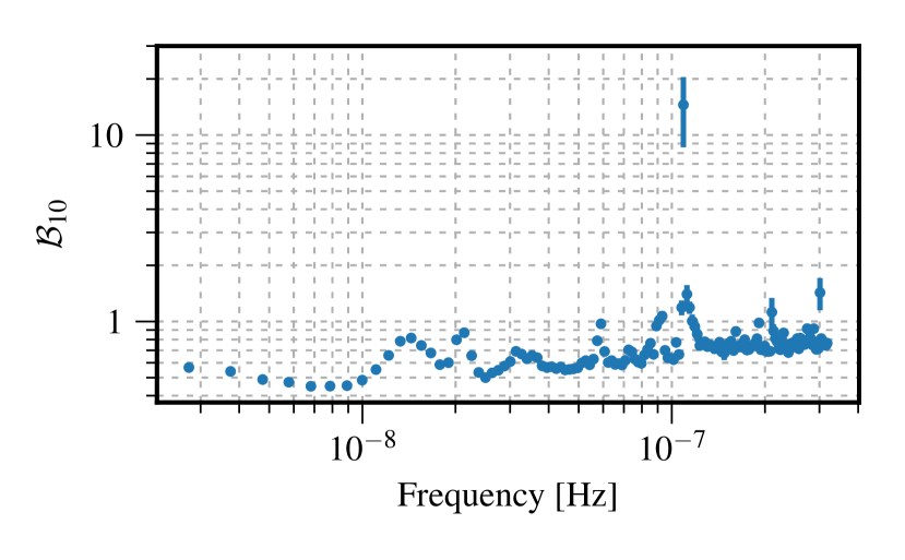
We performed detection searches for GWs from individual circular SMBHBs on the 11-year data set. Figure 1 shows the Bayes factors for each frequency, marginalized over the sky location. We did not find strong evidence for GWs in the 11-year data set. The largest Bayes factor was at , for which . For all other frequencies, the Bayes factors were between and , indicating no evidence of GWs in the data.
We also used the -statistic to determine the significance of a GW signal. Figure 2 shows the -statistic as a function of , and the corresponding FAP as computed from Eq. (28). There are no frequencies for which the FAP lies below our detection threshold of . At the GW frequency that maximizes , the total FAP for the search as computed from Eq. (29) is . Thus we concluded that the frequentist analyses also found that the 11-year data set does not contain significant evidence for GWs.
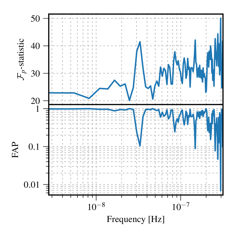
Although the detection search at found a higher Bayes factor than any of the other values of , we emphasize that the Bayes factor is not high enough to claim a detection. A Bayes factor of 15 means 15:1 odds for the presence of a GW signal; similarly, at this frequency the -statistic corresponds to , or signal-to-noise ratio (S/N) of 1.2. Neither of these metrics support the claim that the data show evidence of GWs. Furthermore, as we discuss in more detail in Sec. 4.3, we determined that most of the evidence for this signal was in the residuals of a single pulsar, J1713+0747, whereas a true GW signal this strong should be seen in many pulsars.
4.2. Upper limit analyses
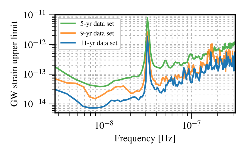
As we did not find strong evidence for GWs from individual circular SMBHBs in the 11-year data set, we placed upper limits on the GW strain. Figure 3 shows the sky-averaged 95% upper limit on the GW strain amplitude. At the most sensitive frequency of , we placed a 95% upper limit on the strain of approximately . We also show the strain upper limits from the 5- and 9-year data sets for comparison. There was an improvement of about a factor of two between the 5-year and 9-year data sets, and more than a factor of two between the 9-year and 11-year data sets. Our upper limit based on the 11-year data set was about 1.4 times lower than that of set by the EPTA based on observations of 6 pulsars observed for up to 17.7 years (Babak et al., 2016; Desvignes et al., 2016). However, a direct comparison between the EPTA results and the results in this paper is complicated by the fact that the analysis in Babak et al. (2016) varied both the white and red noise, whereas our analysis varied only the red noise and fixed the white noise. Our upper limit is also about a factor of 2 lower than that of set by the PPTA using their Data Release 1 (Zhu et al., 2014; Manchester et al., 2013)
We note that there is an increase in the strain upper limit from the 9-year data set at around ; however, there is not a significant Bayes factor at this frequency (). Furthermore, this “bump” in the spectrum is not present in the 11-year data set. If it were caused by a GW, the significance should have increased in the 11-year data set. As discussed in more detail in Sec. 4.3, this increase in the strain upper limit is due to an unmodeled signal in a single pulsar, PSR J06130200.
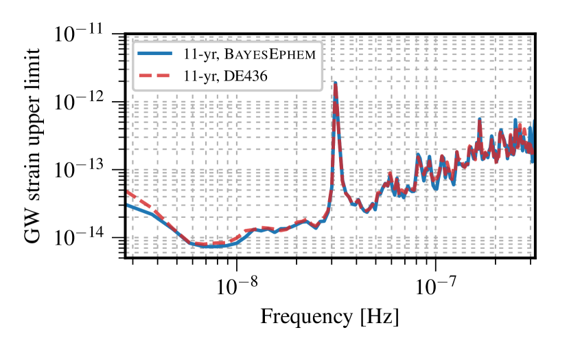
In Figure 4, we compare the sky-averaged strain upper limits computed with and without BayesEphem, which allows for uncertainties in the SSE. Including BayesEphem in our model resulted in a lower strain upper limit for , but did not affect the strain upper limit at higher frequencies. This was expected since BayesEphem primarily augments the orbit of Jupiter, which has an orbital period of 12 years.
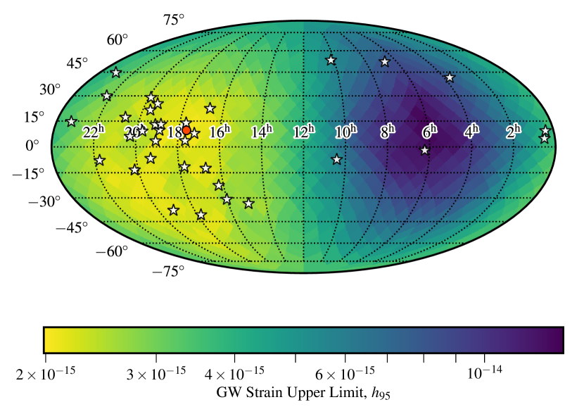
Our sensitivity to individual sources varied significantly with the angular position of the source due to having a finite number of pulsars distributed unevenly across the sky. Figure 5 shows the 95% upper limit on the GW strain for as a function of sky position, plotted in equatorial coordinates. The upper limit varies from at the most sensitive sky location to at the least sensitive sky location.
4.3. “Dropout” analyses
Our searches of the NANOGrav 9-yr and 11-yr data sets found two low-S/N signals. In order to identify their sources, we introduced a new type of analysis that used “dropout” parameters to determine how much each individual pulsar contributed to these signals. In a dropout analysis, the model for a pulsar’s residuals [Eq. (1)] is modified so that the GW signal could be turned on or off in each individual pulsar:
| (30) |
where . The GW parameters were held fixed at the values that maximized the likelihood of a standard GW search, and dropout parameters were introduced into the signal model, which were drawn from a uniform prior between 0 and 1. These parameters determined whether the signal was turned on or off in a particular pulsar:
| (31) |
where sets the prior on whether the signal should be included in a pulsar. For the analyses in this paper, we used , meaning that the prior assumed it was equally likely that the GW be turned on or off. At each iteration of the MCMC, the astrophysical properties of the GW were fixed, and the only thing that varied was which pulsars’ residuals contained the GW signal. The posteriors of the dropout parameters indicated how much support there was for the GW in each pulsar.
The dropout method tests the robustness of the correlations in the signal by determining whether evidence for the signal comes from correlations between multiple pulsars, or it only originates from a single pulsar. It is similar to the dropout technique in neural networks, where units are randomly dropped during training in order to strengthen the network (Srivastava et al., 2014). This method is also similar to jackknife resampling (Efron & Stein, 1981); however, in jackknifing, samples are removed in order to estimate the bias in parameter estimation, whereas in dropout analyses the parameter values are held fixed, and the dropout parameters indicate how much each pulsar is biasing the parameter estimation. An upcoming paper will further describe and develop this method (Vigeland et al., 2019)
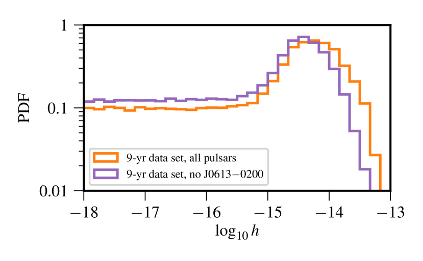
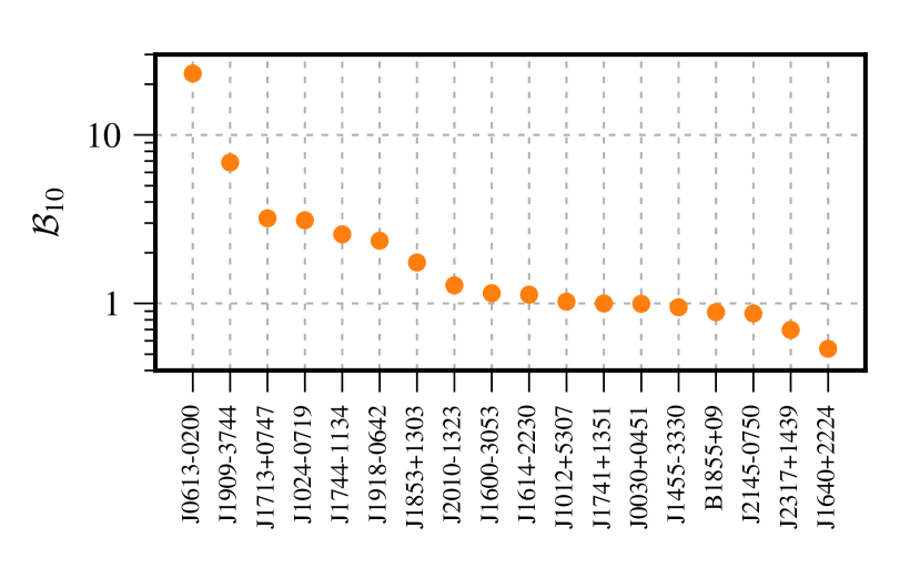
We performed two dropout analyses. The first was on the 9-yr data set at . The analysis of the 9-year data set found an increase in the 95% strain upper limit at compared to the upper limits at neighboring frequencies. Furthermore, as shown in Figure 6, we found that the strain upper limit decreased significantly when PSR J06130200 was removed from the 9-year data set. However, there was very little difference in the Bayes factor: with all pulsars, and excluding PSR J06130200. Figure 7 shows the results of a dropout analysis. We fixed the GW signal parameters to the best-fit values from a detection analysis including all pulsars, and only allowed the dropout parameters to vary. We set , so that there was an equal prior probability of the signal being included or excluded in the model for each pulsar’s residuals. PSR J06130200 had the largest Bayes factor while all other pulsars had Bayes factors of order 1, from which we concluded that the increase in the strain upper limit at was caused by an unmodeled non-GW signal in PSR J06130200. We have applied advanced noise modeling techniques to this pulsar, using more complex models for the red noise, and modeling time-dependent variations in the dispersion as a Gaussian process rather than with DMX. These results will be discussed in an upcoming paper.
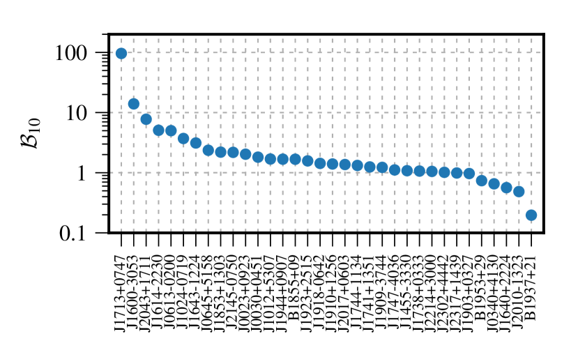
We also performed a dropout analysis on the 11-yr data set at , for which the detection searches had found . Figure 8 shows the Bayes factors for each pulsar’s dropout parameter. We found that PSR J1713+0747 had the strongest Bayes factor for including a GW signal at this frequency, with , indicating that most of the evidence for this signal comes from the residuals of PSR J1713+0747. We did not perform an analysis removing PSR J1713+0747 because it is one of the most sensitive pulsars in the NANOGrav PTA, and removing it always decreases our sensitivity to GWs. Since J1713+0747 significantly contributes to every GW analysis, it is unsurprising that noise in this pulsar can be confused for a GW. A noise analysis of J1713+0747 is underway using the advanced noise modeling techniques that were also applied to J06130200, and the results will be discussed in an upcoming paper. Future CW analyses of PTA data will be able to definitively determine the source of this signal with additional timing data and the incorporation of advanced noise modeling techniques into the data analysis pipeline.
5. Limits on Astrophysical Properties of Nearby SMBHBs
In this section, we discuss what we can infer about the astrophysical properties of nearby SMBHBs from our limits on the GW strain. We used the 95% upper limits on the GW strain to place 95% lower limits on the distance to SMBHBs using Eq. (21) for a given chirp mass. Figure 9 shows the 95% lower limit on the distances to individual SMBHBs as a function of sky position, plotted in equatorial coordinates, for sources with and . The limits on the luminosity distance varied by a factor of 7 between the most-sensitive and least-sensitive sky locations. At the most-sensitive sky location, we found for SMBHBs with and for SMBHBs with .
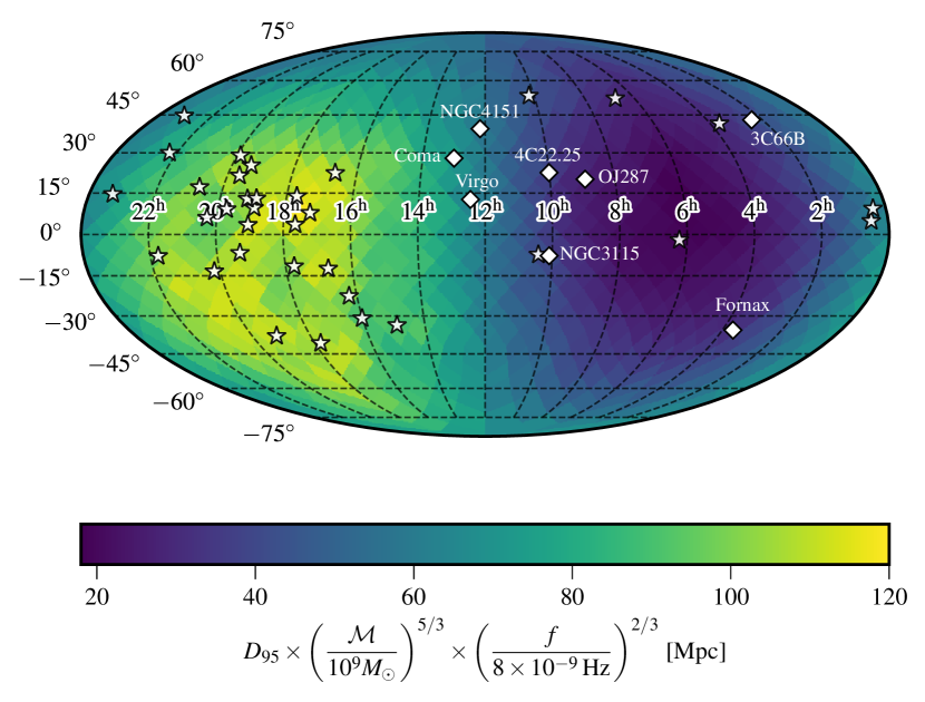
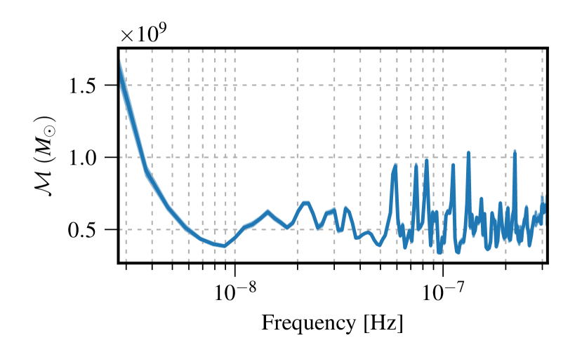
Figure 10 shows the limits on the chirp masses of any SMBHBs in the nearby Virgo Cluster, which is at a distance of . We found that there are no SMBHBs in the Virgo Cluster with emitting GWs in the PTA band. Furthermore, there are no SMBHBs with emitting GWs with . These chirp-mass limits imply that none of the galaxies NGC 4472 (estimated black hole mass of ; Rusli et al. 2013), NGC 4486 (estimated black hole mass of ; Gebhardt et al. 2011), or NGC 4649 (estimated black hole mass of ; Shen & Gebhardt 2010) could contain binaries emitting GWs in this frequency range.
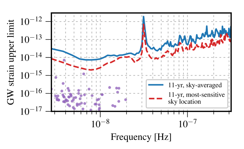
In order to assess how likely we were to have detected a SMBHB given our current sensitivity, we compared our strain upper limit curves to simulations of nearby SMBHBs. A similar technique was introduced in Babak et al. (2016) to estimate the detection probability from the strain upper limit curve. We used simulated populations of SMBHBs from Mingarelli et al. (2017), which are based on galaxies in the Two Micron All-Sky Survey (2MASS; Skrutskie et al. 2006) and merger rates from the Illustris cosmological simulation project (Genel et al., 2014; Rodriguez-Gomez et al., 2015). We estimated the number of detectable sources as the number lying above our sky-averaged 95% strain upper limit curve. Figure 11 shows the loudest GW sources for a sample realization, plotted alongside our 95% strain upper limit curve. We show both the sky-averaged strain upper limit curve (solid, blue line) and the strain upper limit curve at the most-sensitive sky location (dashed, red line). For this particular simulation, none of the sources were above the sky-averaged strain upper limit curve; therefore, we concluded there were no detectable sources in this particular realization. Out of 75,000 realizations of the local Universe, 34 contained a source that lay above the sky-averaged strain upper limit curve (i.e., 0.045% of realizations contained an observable SMBHB), from which we concluded that our non-detection was unsurprising given our current sensitivity. We point out, though, that our sensitivity varies significantly with sky location, and therefore some sources that are below the sky-averaged strain upper limit curve may be detectable depending on their sky locations. In our simulations, we found that a GW source lay above the strain upper limit curve at the most-sensitive sky location in 918 realizations (1.22%).
6. Summary and Conclusions
We searched the NANOGrav 11-year data set for GWs from individual circular SMBHBs. As we found no strong evidence for GWs in our data, we placed limits on the GW strain. We determined that the 11-year data set was most sensitive to , for which the sky-averaged strain upper limit was . We produced sky maps of the GW strain upper limit at . At the most sensitive sky location, we placed a strain upper limit of . These results are the first limits on GWs from individual sources to be robust to uncertainties in the SSE due to the incorporation of BayesEphem in our model. As shown in Fig. 4, uncertainty in the SSE only affects our sensitivity to GWs for .
We introduced a new detection technique that uses “dropout” parameters to determine the significance of a common signal in each individual pulsar. We applied this technique to two low-S/N signals found in the 9-year and 11-year data sets, and identified the pulsars contributing the most to these signals. This technique is currently being used within NANOGrav in other GW searches, and a methods paper developing this technique is underway. Determining the physical processes causing these low-S/N signals is beyond the scope of this paper. Advanced noise analyses of all the pulsars in the NANOGrav PTA are underway, using more complicated models for the red noise and incorporating models for time-variations in the dispersion measure, and the methods and results will be the subject of an upcoming paper.
We used our strain upper limits to place lower limits on the luminosity distance to individual SMBHBs. At the most sensitive sky location, we placed a limit of for and for . Our non-detection of GWs was not surprising given our current sensitivity limits. Using simulated populations of nearby SMBHBs from Mingarelli et al. (2017), we found that only 34 out of 75,000 realizations of the local Universe contained a SMBHB whose GW strain lay above our sky-averaged 95% upper limit curve. These simulations also supported the conclusion that the two low-S/N signals found in the 9-year and 11-year data sets were not GW signals.
Although we have not yet made a positive detection of GWs from individual SMBHBs, the NANOGrav PTA is sensitive enough to place interesting limits on such sources. Based on our non-detection of GWs, we have determined that there are no SMBHBs in the Virgo Cluster with emitting GWs in the PTA band. Furthermore, our sensitivity to GWs from individual SMBHBs will continue to improve as we increase our observation times, add MSPs to our array, and develop improved pulsar noise models.
Appendix A Jump proposals from empirical distributions
In our data analysis pipelines, we computed the posterior distributions using MCMC algorithms, which explore parameter space through a random walk. The CW search for the 11-year data set included 154 parameters: 7 common GW parameters, 68 pulsar-term GW parameters, 68 pulsar red noise parameters, and 11 BayesEphem parameters. Exploring such a large parameter space is computationally intensive, and many iterations are required to burn-in the parameters and ensure the chains have converged. Jump proposals determine how proposed samples are generated, and using particularly good jump proposals can significantly decrease the burn-in and convergence time. Appendix C of NG5b discusses the jump proposals used in the CW search of the NANOGrav 5-year data set, which were also used in the analyses described in this paper.
In the course of analyzing the 11-year data set, we introduced a new type of jump proposal for the pulsars’ red noise parameters and the BayesEphem parameters. These jump proposals chose new parameter values by drawing from empirical distributions based on the posteriors from an initial Bayesian analysis searching over all of the pulsars that included only the pulsars’ red noise and BayesEphem; i.e. excluding any GW term. These jump proposals do not alter the likelihood or the priors – they ensure that the sampler is choosing new parameters that have a high probability of improving the fit, but they do not affect the probability that the new parameter values will be accepted or rejected.
This initial pilot run included only 79 parameters, and therefore the red noise and BayesEphem parameters burned-in relatively quickly. We constructed the empirical distributions from histograms of the posteriors, adding one sample to all bins so that the probability density function was nonzero at every point in the prior. For the red noise parameters, we constructed 2-dimensional empirical distributions for the amplitude and spectral index for each pulsar. For the BayesEphem parameters, we constructed 1-dimensional empirical distributions for each of the six Jupiter orbital elements, which describe perturbations to Jupiter’s orbit.
We have found that including jumps that draw from the empirical distributions to the MCMC dramatically reduces the number of samples needed for the chains to burn-in and converge because the red-noise and BayesEphem parameters converge almost immediately. Efficiently sampling the pulsars’ red noise parameters will become increasingly important as the number of pulsars in our PTA increase, as each pulsar added to the PTA adds two red noise parameters and two pulsar-term parameters to the model.
References
- Arzoumanian et al. (2014) Arzoumanian, Z., Brazier, A., Burke-Spolaor, S., et al. 2014, ApJ, 794, 141
- Arzoumanian et al. (2015) —. 2015, ApJ, 813, 65
- Arzoumanian et al. (2016) —. 2016, ApJ, 821, 13
- Arzoumanian et al. (2018a) —. 2018a, ApJS, 235, 37
- Arzoumanian et al. (2018b) Arzoumanian, Z., Baker, P. T., Brazier, A., et al. 2018b, ApJ, 859, 47
- Babak et al. (2016) Babak, S., Petiteau, A., Sesana, A., et al. 2016, MNRAS, 455, 1665
- Blanco-Pillado et al. (2018) Blanco-Pillado, J. J., Olum, K. D., & Siemens, X. 2018, Physics Letters B, 778, 392
- Burke-Spolaor et al. (2018) Burke-Spolaor, S., Taylor, S. R., Charisi, M., et al. 2018, arXiv e-prints, arXiv:1811.08826
- Burt et al. (2011) Burt, B. J., Lommen, A. N., & Finn, L. S. 2011, ApJ, 730, 17
- Caballero et al. (2018) Caballero, R. N., Guo, Y. J., Lee, K. J., et al. 2018, MNRAS, 481, 5501
- Caprini et al. (2010) Caprini, C., Durrer, R., & Siemens, X. 2010, Phys. Rev. D, 82, 063511
- Chen et al. (2017) Chen, S., Middleton, H., Sesana, A., Del Pozzo, W., & Vecchio, A. 2017, MNRAS, 468, 404
- Christy et al. (2014) Christy, B., Anella, R., Lommen, A., et al. 2014, ApJ, 794, 163
- Corbin & Cornish (2010) Corbin, V., & Cornish, N. J. 2010, ArXiv e-prints, arXiv:1008.1782 [astro-ph.HE]
- Cordes (2013) Cordes, J. M. 2013, Classical and Quantum Gravity, 30, 224002
- Damour & Vilenkin (2001) Damour, T., & Vilenkin, A. 2001, Phys. Rev. D, 64, 064008
- Demorest et al. (2013) Demorest, P. B., Ferdman, R. D., Gonzalez, M. E., et al. 2013, ApJ, 762, 94
- Desvignes et al. (2016) Desvignes, G., Caballero, R. N., Lentati, L., et al. 2016, MNRAS, 458, 3341
- Dickey (1971) Dickey, J. M. 1971, The Annals of Mathematical Statistics, 42, 204
- Dolch et al. (2014) Dolch, T., Lam, M. T., Cordes, J., et al. 2014, ApJ, 794, 21
- Efron & Stein (1981) Efron, B., & Stein, C. 1981, Ann. Statist., 9, 586
- Ellis & van Haasteren (2017a) Ellis, J., & van Haasteren, R. 2017a, jellis18/PAL2: PAL2
- Ellis & van Haasteren (2017b) —. 2017b, jellis18/PTMCMCSampler: Official Release
- Ellis et al. (2012) Ellis, J. A., Siemens, X., & Creighton, J. D. E. 2012, ApJ, 756, 175
- Ellis et al. (2017) Ellis, J. A., Vallisneri, M., Taylor, S. R., & Baker, P. T. 2017, https://github.com/nanograv/enterprise: enterprise
- Folkner & Park (2016) Folkner, W. M., & Park, R. S. 2016, JPL planetary and Lunar ephemeris DE436, Tech. rep., Jet Propulsion Laboratory, Pasadena, CA, https://naif.jpl.nasa.gov/pub/naif/JUNO/kernels/spk/de436s.bsp.lbl
- Gebhardt et al. (2011) Gebhardt, K., Adams, J., Richstone, D., et al. 2011, ApJ, 729, 119
- Genel et al. (2014) Genel, S., Vogelsberger, M., Springel, V., et al. 2014, MNRAS, 445, 175
- Grishchuk (2005) Grishchuk, L. P. 2005, Physics Uspekhi, 48, 1235
- Hobbs (2013) Hobbs, G. 2013, Classical and Quantum Gravity, 30, 224007
- Holgado et al. (2018) Holgado, A. M., Sesana, A., Sandrinelli, A., et al. 2018, MNRAS, 481, L74
- Jenet et al. (2004) Jenet, F. A., Lommen, A., Larson, S. L., & Wen, L. 2004, ApJ, 606, 799
- Jones et al. (2017) Jones, M. L., McLaughlin, M. A., Lam, M. T., et al. 2017, ApJ, 841, 125
- Kelley et al. (2018) Kelley, L. Z., Blecha, L., Hernquist, L., Sesana, A., & Taylor, S. R. 2018, MNRAS, 477, 964
- Lam et al. (2016) Lam, M. T., Cordes, J. M., Chatterjee, S., et al. 2016, ApJ, 821, 66
- Lam et al. (2017) —. 2017, ApJ, 834, 35
- Lasky et al. (2016) Lasky, P. D., Mingarelli, C. M. F., Smith, T. L., et al. 2016, Physical Review X, 6, 011035
- Lee et al. (2011) Lee, K. J., Wex, N., Kramer, M., et al. 2011, MNRAS, 414, 3251
- Manchester et al. (2013) Manchester, R. N., Hobbs, G., Bailes, M., et al. 2013, Publications of the Astronomical Society of Australia, 30, e017
- McLaughlin (2013) McLaughlin, M. A. 2013, Classical and Quantum Gravity, 30, 224008
- Middleton et al. (2018) Middleton, H., Chen, S., Del Pozzo, W., Sesana, A., & Vecchio, A. 2018, Nature Communications, 9, 573
- Mingarelli et al. (2017) Mingarelli, C. M. F., Lazio, T. J. W., Sesana, A., et al. 2017, Nature Astronomy, 1, 886
- Ölmez et al. (2010) Ölmez, S., Mandic, V., & Siemens, X. 2010, Phys. Rev. D, 81, 104028
- Rodriguez-Gomez et al. (2015) Rodriguez-Gomez, V., Genel, S., Vogelsberger, M., et al. 2015, MNRAS, 449, 49
- Rosado et al. (2015) Rosado, P. A., Sesana, A., & Gair, J. 2015, MNRAS, 451, 2417
- Rusli et al. (2013) Rusli, S. P., Thomas, J., Saglia, R. P., et al. 2013, AJ, 146, 45
- Schutz & Ma (2016) Schutz, K., & Ma, C.-P. 2016, MNRAS, 459, 1737
- Sesana (2013) Sesana, A. 2013, Classical and Quantum Gravity, 30, 224014
- Sesana et al. (2004) Sesana, A., Haardt, F., Madau, P., & Volonteri, M. 2004, ApJ, 611, 623
- Sesana et al. (2018) Sesana, A., Haiman, Z., Kocsis, B., & Kelley, L. Z. 2018, ApJ, 856, 42
- Sesana & Vecchio (2010) Sesana, A., & Vecchio, A. 2010, Phys. Rev. D, 81, 104008
- Shen & Gebhardt (2010) Shen, J., & Gebhardt, K. 2010, ApJ, 711, 484
- Skrutskie et al. (2006) Skrutskie, M. F., Cutri, R. M., Stiening, R., et al. 2006, AJ, 131, 1163
- Srivastava et al. (2014) Srivastava, N., Hinton, G., Krizhevsky, A., Sutskever, I., & Salakhutdinov, R. 2014, Journal of Machine Learning Research, 15, 1929
- Taylor et al. (2016) Taylor, S. R., Huerta, E. A., Gair, J. R., & McWilliams, S. T. 2016, ApJ, 817, 70
- Taylor et al. (2017) Taylor, S. R., Simon, J., & Sampson, L. 2017, Physical Review Letters, 118, 181102
- Tiburzi et al. (2016) Tiburzi, C., Hobbs, G., Kerr, M., et al. 2016, MNRAS, 455, 4339
- van Haasteren & Vallisneri (2015) van Haasteren, R., & Vallisneri, M. 2015, Mon. Not. Roy. Astron. Soc., 446, 1170
- Verbiest et al. (2012) Verbiest, J. P. W., Weisberg, J. M., Chael, A. A., Lee, K. J., & Lorimer, D. R. 2012, ApJ, 755, 39
- Verbiest et al. (2016) Verbiest, J. P. W., Lentati, L., Hobbs, G., et al. 2016, MNRAS, 458, 1267
- Vigeland et al. (2019) Vigeland, S. J., Vallisneri, M., & Taylor, S. R. 2019, in preparation
- Wahlquist (1987) Wahlquist, H. 1987, General Relativity and Gravitation, 19, 1101
- Yardley et al. (2010) Yardley, D. R. B., Hobbs, G. B., Jenet, F. A., et al. 2010, MNRAS, 407, 669
- Zhu et al. (2014) Zhu, X.-J., Hobbs, G., Wen, L., et al. 2014, MNRAS, 444, 3709