Variational Self-attention Model for Sentence Representation
Abstract
This paper proposes a variational self-attention model (VSAM) that employs variational inference to derive self-attention. We model the self-attention vector as random variables by imposing a probabilistic distribution. The self-attention mechanism summarizes source information as an attention vector by a weighted sum, where the weights are a learned probabilistic distribution. Compared with conventional deterministic counterpart, the stochastic units incorporated by VSAM enable multi-modal distributions of attention. Furthermore, by marginalizing over latent variables, VSAM is experimentally more robust against overfitting. Experiments on the stance detection task demonstrate the superiority of our method.
1 Background
1.1 Sentence representation
A sentence usually consists of a sequence of discrete words or tokens , where can be a one-hot vector with the dimension equal to the number of unique tokens in the vocabulary. Pre-trained distributed word embeddings, such as Word2vec [6] and GloVe [8], have been developed to transform into a lower-dimensional vector representation , whose dimension is much smaller than . Thus, a sentence can be encoded in a more dense representation . The encoding process can be written as: , where is the transformation matrix. In the areas of natural language processing, the majority of deep learning methods (e.g. RNN and CNN) take as the input and generate a compact vector representation for a sentence: , where indicates a RNN model. These methods consider the semantic dependencies between and its context and hence believe that summarizes the semantic information of the entire sentence.
1.2 Self-attention
The attention mechanism [1, 9] has been proposed as an alignment score between elements from two vector representations. Specifically, given the vector representation of a query and a token sequence , the attention mechanism is to compute the alignment score between and .
Self-attention [7] is a special case of the attention mechanism, where is replaced with a token embedding from the input sequence itself. Self-attention is a method of encoding sequences of vectors by relating these vectors to each-other based on pairwise similarities. It measures the dependency between each pair of tokens, and , from the same input sequence: , where indicates a self-attention implementation.
Self-attention is very expressive and flexible for both long-term and local dependencies, which used to be respectively modeled by RNN and CNN. Moreover, the self-attention mechanism has fewer parameters and faster convergence than RNN. Recently, a variety of NLP tasks have experienced improvement brought by the self-attention mechanism.
1.3 Neural variational inference
Latent variable modeling is popular for many NLP tasks [5, 2]. It populates hidden representations to a region (in stead of a single point), making it possible to generate diversified data from the vector space or even control the generated samples. It is non-trivial to carry out effective and efficient inference for complex and deep models. Training neural networks as powerful function approximators through backpropagation has given rise to promising frameworks to latent variable modeling [3, 4].
The modeling process builds a generative model and an inference model. A generative model is to construct the joint distribution and somehow capture the dependencies between variables. The latent variable the can be seen as stochastic units in the generative model. The observed input and output nodes of are denoted as and respectively. Hence the joint distribution of the generative model is:
| (1) |
where parameters the generative distributions and . The variational lower bound is:
| (2) |
In order to derive the evidence lower bound, the variational distribution should approach the true posterior distribution . A parametrized diagonal Gaussian distribution is employed as .
The inference model is to derive the variational distribution that approaches the posterior distribution of latent variables given observed variables. The procedure to construct the inference model is:
-
1.
Construct vector representations of the observed variables: , .
-
2.
Assemble a joint distribution: .
-
3.
Parameterize the variational distribution over the latent variables: , .
and are implemented as deep neural networks; can be an multi-layer perceptron that fully connects the vector representations of the conditioning variables; is a matrix transformation which computes the Gaussian distribution parameters. Sampling from the variational distribution, i.e., , allows to conduct stochastic back-propagation to optimize the evidence lower bound.
During training, the parameter of the generative model and the parameters of the inference model are updated by stochastic back-propagation based on samples drawn from . Let denote the total number of samples. The gradients w.r.t. , are in the form of:
| (3) |
As about the gradients w.r.t. parameters , we use the reparameterization trick and sample . can be updated by back-propagation of the gradients w.r.t. and :
| (4) | |||
| (5) |
2 Variational Self-attention Model
In this paper we propose a Variational Self-attention Model (VSAM) that employs variational inference to learn self-attention. In doing so the model will implement a stochastic self-attention learning mechanism instead of the conventional deterministic one, and obtain a more salient inner-sentence semantic relationship. The framework of the model is shown in Figure 1.
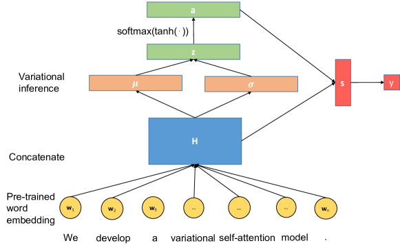
Suppose we have a sentence , where is the pre-trained word embedding and is the number of words in the sentence. We concatenate the word embeddings to form a matrix , where is the dimension of the word embedding. We aim to learn semantic dependencies between every pair of tokens through self-attention. Instead of using the deterministic self-attention vector, VSAM employs a latent distribution to model semantic dependencies, which is a parameterized diagonal Gaussian . Therefore, the self-attention model extracts an attention vector based on the stochastic vector .
The diagonal Gaussian conditional distribution can be calculated as follows:
| (6) | |||
| (7) | |||
| (8) |
For each sentence embedding , the neural network generates the corresponding parameters and that parametrize the latent self-attention distribution over the entire sentence semantics.
The self-attention vector can then be derived as: . The final sentence vector representation is the sentence embedding matrix weighted by the self-attention vector as: , where . For the downstream application with expected output , the conditional probability distribution can be modeled as: . As for the inference network, we follow the neural variational inference framework and construct a deep neural network as the inference network. We use and to compute as: . According to the joint representation , we can then generate the parameters and , which parameterize the variational distribution over the sentence semantics :
| (9) | |||
| (10) |
To emphasize, although both and are modeled as parameterized Gaussian distributions, as an approximation only functions during inference by producing samples to compute the stochastic gradients, while is the generative distribution that generates the samples for predicting . To maximize the log-likelihood we use the variational lower bound. Based on the samples , the variational lower bound can be derived as
| (11) | ||||
The generative model parameters and the inference model parameters are updated jointly according to their stochastic gradients. In this case, can be analytically computed during the training process.
3 Experiments
| Stance | Training | Test | ||
|---|---|---|---|---|
| Number | Percentage | Number | Percentage | |
| agree | 03,678 | 07.36 | 1,903 | 07.49 |
| disagree | 00840 | 01.68 | 0697 | 02.74 |
| discuss | 08,909 | 17.83 | 4,464 | 17.57 |
| unrelated | 36,545 | 73.13 | 18,349 | 72.20 |
| 49,972 | 25,413 | |||
In this section, we describe our experimental setup. The task we address is to detect the stance of a piece of text towards a claim as one of the four classes: agree, disagree, discuss and unrelated [10]. Experiments are conducted on the FNC-1 official dataset 111 https://github.com/FakeNewsChallenge/fnc-1. The dataset are split into training and testing subsets, respectively; see Table 1 for statistics of the split. We report classification accuracy and micro F1 metrics on test dataset for each type of stances.
Baselines for comparisons include: (1) Average of Word2vec Embedding refers to sentence embedding by averaging vectors of each word based on Word2vec. (2) CNN-based Sentence Embedding refers to sentence embedding by inputting the Word2vec embedding of each word to a convolutional neural network. (3) Self-attention Sentence Embedding refers to sentence embedding by calculating self-attention based sentence embedding, without variational inference.
| Model | Accuracy (%) | Micro F1(%) | |||
|---|---|---|---|---|---|
| agree | disagree | discuss | unrelated | ||
| Average of Word2vec Embedding | 12.43 | 01.30 | 43.32 | 74.24 | 45.53 |
| CNN-based Sentence Embedding | 24.54 | 05.06 | 53.24 | 79.53 | 81.72 |
| RNN-based Sentence Embedding | 24.42 | 05.42 | 69.05 | 65.34 | 78.70 |
| Self-attention Sentence Embedding | 23.53 | 04.63 | 63.59 | 80.34 | 80.11 |
| Our model | 28.53 | 10.43 | 65.43 | 82.43 | 83.54 |
Table 2 shows a comparison of the detection performance. As for the micro F1 evaluation metric, our model achieves the highest performance (83.54%) on the FNC-1 testing subset. The average method can lose emphasis or key word information in a claim; the CNN-based method can only capture local dependency among the text with limit to the filter size; the RNN-based method can obtain semantic relationship in a sequential manner. Differently, the self-attention method is able to combine embedding information between each pair of words, which means more accurate semantic matching of the claim and the piece of text. Compared with the deterministic self-attention, our method is a stochastic approach that is experimentally proven to better integrate each word embedding.
4 Conclusion
We propose a variational self-attention model (VSAM) that builds a self-attention vector as random variables by imposing a probabilistic distribution. Compared with conventional deterministic counterpart, the stochastic units incorporated by VSAM allow multi-modal attention distributions. Furthermore, by marginalizing over the latent variables, VSAM is more robust against overfitting, which is important for small datasets. Experiments on the stance detection task demonstrate the superiority of our method.
Acknowledgments
This project was funded by the EPSRC Fellowship titled "Task Based Information Retrieval", grant reference number EP/P024289/1.
References
- [1] D. Bahdanau, K. Cho, and Y. Bengio. Neural machine translation by jointly learning to align and translate. CoRR, abs/1409.0473, 2014.
- [2] H. Bahuleyan, L. Mou, O. Vechtomova, and P. Poupart. Variational attention for sequence-to-sequence models. In Proceedings of the 27th International Conference on Computational Linguistics, COLING 2018, Santa Fe, New Mexico, USA, August 20-26, 2018, pages 1672–1682, 2018.
- [3] Z. Lin, M. Feng, C. N. dos Santos, M. Yu, B. Xiang, B. Zhou, and Y. Bengio. A structured self-attentive sentence embedding. CoRR, abs/1703.03130, 2017.
- [4] R. Luo, W. Zhang, X. Xu, and J. Wang. A neural stochastic volatility model. In Proceedings of the Thirty-Second AAAI Conference on Artificial Intelligence, New Orleans, Louisiana, USA, February 2-7, 2018, 2018.
- [5] Y. Miao, L. Yu, and P. Blunsom. Neural variational inference for text processing. In Proceedings of the 33nd International Conference on Machine Learning, ICML 2016, New York City, NY, USA, June 19-24, 2016, pages 1727–1736, 2016.
- [6] T. Mikolov, I. Sutskever, K. Chen, G. S. Corrado, and J. Dean. Distributed representations of words and phrases and their compositionality. In Advances in Neural Information Processing Systems 26: 27th Annual Conference on Neural Information Processing Systems 2013. Proceedings of a meeting held December 5-8, 2013, Lake Tahoe, Nevada, United States., pages 3111–3119, 2013.
- [7] A. P. Parikh, O. Täckström, D. Das, and J. Uszkoreit. A decomposable attention model for natural language inference. In Proceedings of the 2016 Conference on Empirical Methods in Natural Language Processing, EMNLP 2016, Austin, Texas, USA, November 1-4, 2016, pages 2249–2255, 2016.
- [8] J. Pennington, R. Socher, and C. D. Manning. Glove: Global vectors for word representation. In Proceedings of the 2014 Conference on Empirical Methods in Natural Language Processing, EMNLP 2014, October 25-29, 2014, Doha, Qatar, A meeting of SIGDAT, a Special Interest Group of the ACL, pages 1532–1543, 2014.
- [9] A. Vaswani, N. Shazeer, N. Parmar, J. Uszkoreit, L. Jones, A. N. Gomez, L. Kaiser, and I. Polosukhin. Attention is all you need. In Advances in Neural Information Processing Systems 30: Annual Conference on Neural Information Processing Systems 2017, 4-9 December 2017, Long Beach, CA, USA, pages 6000–6010, 2017.
- [10] Q. Zhang, E. Yilmaz, and S. Liang. Ranking-based method for news stance detection. In Companion of the The Web Conference 2018 on The Web Conference 2018, pages 41–42. International World Wide Web Conferences Steering Committee, 2018.