Convergence in Orlicz spaces by means of the multivariate max-product neural network operators of the Kantorovich type and applications

Abstract

In this paper, convergence results in a multivariate setting have been proved for a family of neural network operators of the max-product type. In particular, the coefficients expressed by Kantorovich type means allow to treat the theory in the general frame of the Orlicz spaces, which includes as particular case the $L^{p}$-spaces. Concrete examples of sigmoidal activation functions are discussed, for the above operators in different cases of Orlicz spaces. Finally, concrete applications to real world cases have been presented in both univariate and multivariate settings. In particular, the case of reconstruction and enhancement of biomedical (vascular) image has been discussed in details. AMS 2010 Mathematics Subject Classification: 41A25, 41A05, 41A30, 47A58 Key words and phrases: sigmoidal function; multivariate max-product neural network operator; Orlicz space; modular convergence; neurocomputing process; data modeling; image processing.

1 Introduction

The study of neural network type operators has been recently investigated by many authors from the theoretical point of view, see e.g., [46, 16, 17, 18, 14].

A particular attention has been reserved to the so-called max-product version of the above operators, which can be useful, for instance, in the applications of probability and fuzzy theory. The introduction of this approach is due to Bede, Coroianu and Gal (see e.g., [20, 21]), and recently they summarized their results in a very complete monograph [12]. In general, the max-product version of a family of linear operators are sub-linear and has better approximation properties: in many cases, the order of convergence is faster with respect to their linear counterparts.

In the present paper, we extend the results proved in [23] to the multivariate frame: the latter is the most suitable when we deal with neural network type approximation. Indeed, neural networks have been introduced in order to study a simple model for the human brain, which is a very complicated structure composed by billions of neurons; this justify the multidimensional form of the neural networks. The behavior of the (artificial) neurons in the neuronal models is regulated by suitable activation functions which must represent the activation and the quite phases of the neurons ([45]). From the mathematical point of view, functions which better represent the latter fact are those with sigmoidal behavior ([39, 40]). A sigmoidal function ([27]) is any measurable function $\sigma:\mathbb{R}\to\mathbb{R}$, such that:

$$\lim_{x\to-\infty}\sigma(x)=0,\quad\quad\mbox{and}\quad\quad\lim_{x\to+\infty}\sigma(x)=1.$$

Problems of interpolation, or more in general, of approximation are related with the topic of training a neural network by sample values belonging to a certain training set: this explain the interest of studying approximation results by means of NN operators in various contexts ([42]).

Indeed, results in this sense have been deeply studied for what concerns various aspects, such as convergence, order of approximation, saturation, and so on ([28, 29, 32]).

Here, we consider the above NN operators, with coefficients expressed by Kantorovich means in a multivariate form. It is well-know that this kind of approach based on Kantorovich-type operators is the most suitable in order to approximate not necessarily continuous data ([22, 2, 11, 33]). For this reason, we study the above operators in the general setting of Orlicz spaces, which is a very general context, which includes, as particular cases, the $L^{p}$-spaces. Moreover, since images are typical examples of discontinuous data, Kantorovich-type operators have been recently applied to image processing, see [6, 7].

From the theoretical results established in the present paper, we obtain, by a unifying approach, a general treatment of the problem of the approximation of both multivariate continuous and not necessarily continuous functions by means of the max-product neural network operators. Further, the results here proved extend to a more general setting those achieved by the authors in [31].

We also provide some concrete applications of the obtained results. In particular, we show how it is possible to reconstruct and even to enhance images by means of the above max-product type operators. The proposed examples involve the biomedical images concerning the vascular apparatus. More precisely, we reconstruct a CT image (computer tomography image) depicting an aneurysm of the abdominal aorta artery. Then, we show how it is possible to reconstruct and also to increase the resolution of a given image by the above operators (without losing information), in fact obtaining a detailed image which can be more useful from the diagnostic point of view.

Further, also applications in case of one-dimensional data modeling have been presented (see, e.g., [37]).

The above mentioned topics give a contribution to an application field which in the last years have been widely studied by means of the use of suitable neural network type models, see e.g., [1, 34].

Now, we give a plan of the paper. In Section 2 the definition of the above operators and their main properties have been recalled, together with some notations and preliminary results. In Section 3 the main convergence results of the paper have been proved. In order to show that the family of multivariate Kantorovich max-product operators are modularly convergent in Orlicz spaces, we adopt the following strategy: (i) we test the norm-convergence for the above operators in case of continuous functions; (ii) we prove a modular inequality for the above operators in $L^{\varphi}$, where $\varphi$ is a convex $\varphi$-function; finally (iii) we obtain the desired results exploiting the modular density of the continuous functions in $L^{\varphi}$. In Section 4 we provided several examples of Orlicz spaces for which the above theory holds, and also some well-known examples of sigmoidal activation functions, while in Section 5 we present the above mentioned real world applications.

2 The multivariate max-product neural network operators of the Kantorovich type

From now on, the symbols $\lfloor\cdot\rfloor$ and $\lceil\cdot\rceil$ will denote respectively the “integer” and the “ceiling” part of a given number. Moreover, we define:

$$\bigvee_{k\in{\cal J}}A_{k}\ :=\ \sup\left\{A_{\underline{k}}\in\mathbb{R},\ \underline{k}\in{\cal J}\right\},$$

for any set of indexes ${\cal J}\subset\mathbb{Z}^{s}$.

Let now $f:\mathcal{R}\to\mathbb{R}$ be a locally integrable and bounded function, where $\mathcal{R}\subset\mathbb{R}^{s}$, is the box-set of the form $\mathcal{R}:=[a_{1},b_{1}]\times[a_{2},b_{2}]\times\dots\times[a_{s},b_{s}]$. Further, let $n\in\mathbb{N}^{+}$ such that $\lceil na_{i}\rceil\leq\lfloor nb_{i}\rfloor-1$, for every $i=1,...,s$.

The multivariate max-product neural network (NN) operators of Kantorovich type (see [31]) activated by the sigmoidal function $\sigma$, are defined by:

$$K^{(M)}_{n}(f,\,\underline{x})\ :=\ \frac{\displaystyle\bigvee_{\underline{k}\in\mathcal{J}_{n}}\left[n^{s}\int_{R^{n}_{\underline{k}}}f\left(\underline{u}\right)\,d\underline{u}\right]\Psi_{\sigma}(n\underline{x}-\underline{k})}{\displaystyle\bigvee_{\underline{k}\in\mathcal{J}_{n}}\Psi_{\sigma}(n\underline{x}-\underline{k})},\hskip 22.76228pt\underline{x}\in\mathcal{R},$$

where:

$$R^{n}_{\underline{k}}\ :=\ \left[\frac{k_{1}}{n},\frac{k_{1}+1}{n}\right]\times\dots\times\left[\frac{k_{s}}{n},\frac{k_{s}+1}{n}\right],$$

for every $\underline{k}\in\mathcal{J}_{n}$, and $\mathcal{J}_{n}$ denotes the set of indexes $\underline{k}\in\mathbb{Z}^{s}$ such that $\lceil na_{i}\rceil\leq k_{i}\leq\lfloor nb_{i}\rfloor-1$, $i=1,...,s$, for every $n\in\mathbb{N}^{+}$ sufficiently large.

Here, the multivariate function $\Psi_{\sigma}:\mathbb{R}^{s}\to\mathbb{R}$ is defined as follows:

$$\Psi_{\sigma}(\underline{x})\ :=\ \phi_{\sigma}(x_{1})\cdot\phi_{\sigma}(x_{2})\dots\cdot\phi_{\sigma}(x_{s}),$$

with $\underline{x}:=(x_{1},x_{2},...,x_{s})\in\mathbb{R}^{s}$, and:

$$\phi_{\sigma}(x)\,:=\,\frac{1}{2}\,[\sigma(x+1)-\sigma(x-1)],\hskip 28.45274ptx\in\mathbb{R},$$

for every non-decreasing sigmoidal function $\sigma:\mathbb{R}\to\mathbb{R}$, which satisfies the following conditions:

• $\sigma(x)-1/2$ is an odd function;

• $\phi_{\sigma}(x)$ is non-decreasing for $x<0$ and non-increasing for $x\geq 0$;

• $\sigma(x)={\cal O}(|x|^{-\alpha})$ as $x\to-\infty$, for some $\alpha>0$.

Let now $f$, $g:\mathcal{R}\to\mathbb{R}$ be bounded functions. The following properties hold for sufficiently large $n\in\mathbb{N}^{+}$ (see [26] for the proof in the one-dimensional case, and [31] in case of functions of several variables):

(a) if $f(\underline{x})\leq g(\underline{x})$, for each $\underline{x}\in\mathcal{R}$, we have $K^{(M)}_{n}(f,\underline{x})\leq K^{(M)}_{n}(g,\underline{x})$, for every $\underline{x}\in\mathcal{R}$ (the operators are monotone);

(b) $K^{(M)}_{n}(f+g,\,\underline{x})\leq K^{(M)}_{n}(f,\underline{x})+K^{(M)}_{n}(g,\underline{x})$, $x\in\mathcal{R}$ (the operators are sub-additive);

(c) $\left|K^{(M)}_{n}(f,\underline{x})-K^{(M)}_{n}(g,\underline{x})\right|\leq K^{(M)}_{n}(|f-g|,\,\underline{x})$, $\underline{x}\in\mathcal{R}$;

(d) $K^{(M)}_{n}(\lambda f,\underline{x})=\lambda K^{(M)}(f,\underline{x})$, $\lambda>0$, $\underline{x}\in\mathcal{R}$ (the operators are positive homogeneous).

In [27, 28] some important properties of the functions $\phi_{\sigma}(x)$ and $\Psi_{\sigma}(\underline{x})$ have been proved. In the following lemma, we recall those that can be useful in order to prove the convergence results for the above operators in Orlicz spaces for functions of several variables.

Lemma 2.1.

$($i$)$ $\phi_{\sigma}(x)\geq 0$ for every $x\in\mathbb{R}$, with $\phi_{\sigma}(2)>0$, and moreover $\displaystyle\lim_{x\to\pm\infty}\phi_{\sigma}(x)=0$;

$($ii$)$ $\phi_{\sigma}(0)\geq\phi_{\sigma}(x)$, for every $x\in\mathbb{R}$, and $\phi_{\sigma}(0)\leq 1/2$. Consequently, $\Psi_{\sigma}(\underline{0})\geq\Psi_{\sigma}(\underline{x})$, for every $\underline{x}\in\mathbb{R}^{s}$, and $\Psi_{\sigma}(\underline{0})\leq 2^{-s}$;

$($iii$)$ $\Psi_{\sigma}(\underline{x})=\mathcal{O}(\|\underline{x}\|_{2}^{-\alpha})$, as $\|\underline{x}\|_{2}\to+\infty$, where $\alpha$ is the positive constant of condition $(\Sigma 3)$, and $\|\cdot\|_{2}$ denotes the usual Euclidean norm of $\mathbb{R}^{s}$;

$($iv$)$ $\Psi_{\sigma}\in L^{1}(\mathbb{R}^{s})$;

$($v$)$ For any fixed $\underline{x}\in\mathcal{R}$, there holds:

$$\bigvee_{\underline{k}\in\mathcal{J}_{n}}\Psi_{\sigma}(n\underline{x}-\underline{k})\ \geq\ [\phi_{\sigma}(2)]^{s}\ >\ 0.$$

Now, we can introduce the general setting in which we will work, i.e., the Orlicz spaces. We begin recalling the following definition.

A function $\varphi:\mathbb{R}^{+}_{0}\to\mathbb{R}^{+}_{0}$ which satisfies the following assumptions:

• $\varphi\left(0\right)=0$, $\varphi\left(u\right)>0$ for every $u>0$;

• $\varphi$ is continuous and non decreasing on $\mathbb{R}^{+}_{0}$;

• $\displaystyle\lim_{u\to+\infty}\varphi(u)\ =\ +\infty$,

is said to be a $\varphi$-function. Let $M({\cal R})$ denotes the set of all (Lebesgue) measurable functions $f:{\cal R}\to\mathbb{R}$. For any fixed $\varphi$-function $\varphi$, it is possible to define the functional $I^{\varphi}:M({\cal R})\to[0,+\infty]$, as follows:

$$I^{\varphi}\left[f\right]:=\int_{{\cal R}}\varphi(\left|f(\underline{x})\right|)\ d\underline{x},\ \hskip 14.22636ptf\in M({\cal R}).$$

The functional $I^{\varphi}$ is called a modular on $M({\cal R})$. Then, we can define the Orlicz space generated by $\varphi$ by the set:

$$L^{\varphi}({\cal R}):=\left\{f\in M\left({\cal R}\right):\ I^{\varphi}[\lambda f]<+\infty,\ \mbox{for\ some}\ \lambda>0\right\}.$$

Now, exploiting the definition of the modular functional $I^{\varphi}$, it is possible to introduce a notion of convergence in $L^{\varphi}({\cal R})$, the so-called modular convergence.

More precisely, a family of functions $(f_{w})_{w>0}\subset L^{\varphi}({\cal R})$ is said modularly convergent to a function $f\in L^{\varphi}({\cal R})$ if:

$$\lim_{w\to+\infty}I^{\varphi}\left[\lambda(f_{w}-f)\right]\ =\ 0,$$ (1)

for some $\lambda>0$. If (1) holds for every $\lambda>0$, we will say that the family $(f_{w})_{w>0}$ is norm convergent to $f$. Obviously, the norm convergence is in general stronger than modular convergence. Both the above definitions become equivalent if and only if the $\varphi$-function $\varphi$, which generates $L^{\varphi}({\cal R})$, satisfies:

$$\varphi(2u)\ \leq\ M\varphi(u),\hskip 22.76228ptu\in\mathbb{R}^{+}_{0}\quad\quad(\Delta_{2}-condition),$$

for some $M>0$.

Finally, if we denote by $C({\cal R})$ the space of all continuous functions $f:{\cal R}\to\mathbb{R}$, it turns out that $C({\cal R})\subset L^{\varphi}({\cal R})$, and moreover, there holds that $C({\cal R})$ is dense in $L^{\varphi}({\cal R})$ with respect to the topology induced by the modular convergence.

Similarly, denoting respectively by $C_{+}({\cal R})$ and $L^{\varphi}_{+}({\cal R})$ the subspaces of $C({\cal R})$ and $L^{\varphi}({\cal R})$ of the non-negative and almost everywhere non-negative functions, respectively, it turns out that also $C_{+}({\cal R})$ is modularly dense in $L^{\varphi}_{+}({\cal R})$.

For more details concerning Orlicz spaces, see e.g., [48, 47, 10, 3, 4, 5, 30, 9].

In conclusion, we recall some well-known convergence result for the operators $K^{(M)}_{n}$, that will be useful in the next sections.

Theorem 2.2 ([31]).

Let $f:\mathcal{R}\to\mathbb{R}^{+}_{0}$ be a given bounded function. Then,

$$\lim_{n\to+\infty}K^{(M)}_{n}(f,\underline{x})\ =\ f(\underline{x}),$$

at any point $\underline{x}\in\mathcal{R}$ of continuity for $f$. Moreover, if $f\in C_{+}(\mathcal{R})$, we have:

$$\lim_{n\to+\infty}\|K^{(M)}_{n}(f,\cdot)\ -\ f(\cdot)\|_{\infty}\ =\ 0.$$

3 Convergence in Orlicz spaces

From now on, we always consider convex $\varphi$-functions $\varphi$. Hence, we begin by proving the following auxiliary result.

Theorem 3.1.

Let $f\in C_{+}({\cal R})$ be fixed. Then, for every $\lambda>0$:

$$\lim_{n\to+\infty}I^{\varphi}\left[\lambda\left(K^{(M)}_{n}(f,\cdot)-f(\cdot)\right)\right]\ =\ 0.$$

Proof.

Let $\varepsilon>0$ be fixed. For every fixed $\lambda>0$, using the convexity of $\varphi$, and in view of Theorem 2.2, we have:

$$I^{\varphi}\left[\lambda\left(K^{(M)}_{n}(f,\cdot)-f(\cdot)\right)\right]\ =\ \int_{\cal R}\varphi\left(\lambda\left|K^{(M)}_{n}(f,\underline{x})-f(\underline{x})\right|\right)\,d\underline{x}$$

$$\leq\ \int_{\cal R}\varphi\left(\lambda\|K^{(M)}_{n}(f,\cdot)-f(\cdot)\|_{\infty}\right)\,d\underline{x}\ \leq\ \int_{\cal R}\varphi\left(\lambda\,\varepsilon\right)\,d\underline{x}\ \leq\ \varepsilon\,\varphi(\lambda)|{\cal R}|,$$

for $n\in\mathbb{N}^{+}$ sufficiently large, where $|{\cal R}|$ denotes the Lebesgue measure of ${\cal R}$. Hence the proof follows since $\varepsilon>0$ is arbitrary. ∎

Theorem 3.1 states that the family $K^{(M)}_{n}f$ is norm convergent to $f\in C_{+}({\cal R})$. Now, we need to prove a modular inequality for the above operators, in the setting of Orlicz spaces.

Theorem 3.2.

For every $f$, $g\in L^{\varphi}_{+}({\cal R})$, and $\lambda>0$, it turns out that:

$$I^{\varphi}\left[\lambda\left(K^{(M)}_{n}(f,\cdot)-K^{(M)}_{n}(g,\cdot)\right)\right]\ \leq\ \|\Psi_{\sigma}\|_{1}\,I^{\varphi}\left[\phi_{\sigma}(2)^{-s}\lambda\,\left(f(\cdot)-g(\cdot)\right)\right],$$

for $n\in\mathbb{N}^{+}$ sufficiently large.

Proof.

Using inequality (c) of $K^{(M)}_{n}$, and Lemma 2.1 (v), we can write what follows:

$$I^{\varphi}\left[\lambda\left(K^{(M)}_{n}(f,\cdot)-K^{(M)}_{n}(g,\cdot)\right)\right]\ =\ \int_{\cal R}\varphi\left(\lambda\left|K^{(M)}_{n}(f,\underline{x})-K^{(M)}_{n}(g,\underline{x})\right|\right)\,d\underline{x}$$

$$\hskip-187.78836pt\leq\ \int_{\cal R}\varphi\left(\lambda\,K^{(M)}_{n}(|f-g|,\underline{x})\right)\,d\underline{x}$$

$$\leq\ \int_{\cal R}\varphi\left(\lambda\,\phi_{\sigma}(2)^{-s}\bigvee_{\underline{k}\in{\cal J}_{n}}\left[n^{s}\int_{R^{n}_{\underline{k}}}|f(\underline{u})-g(\underline{u})|\,d\underline{u}\right]\Psi_{\sigma}(n\underline{x}-\underline{k})\right)\,d\underline{x}.$$

Now, we observe that:

$$\varphi\left(\bigvee_{k\in{\cal J}}A_{k}\right)\ =\ \bigvee_{k\in{\cal J}}\varphi\left(A_{k}\right),$$ (2)

for any finite set of indexes ${\cal J}\subset\mathbb{Z}^{s}$, since $\varphi$ is non-decreasing. Thus, using (2), the convexity of $\varphi$, Lemma 2.1 (ii), and the Jensen’s inequality (see, e.g., [24]), we obtain:

$$\hskip-142.26378ptI^{\varphi}\left[\lambda\left(K^{(M)}_{n}(f,\cdot)-K^{(M)}_{n}(g,\cdot)\right)\right]\$$

$$\leq\ \int_{\cal R}\bigvee_{\underline{k}\in{\cal J}_{n}}\varphi\left(\lambda\,\phi_{\sigma}(2)^{-s}\left[n^{s}\int_{R^{n}_{\underline{k}}}|f(\underline{u})-g(\underline{u})|\,d\underline{u}\right]\Psi_{\sigma}(n\underline{x}-\underline{k})\right)\,dx$$

$$\leq\ \int_{\cal R}\bigvee_{\underline{k}\in{\cal J}_{n}}\Psi_{\sigma}(n\underline{x}-\underline{k})\,\varphi\left(\lambda\,\phi_{\sigma}(2)^{-s}\left[n^{s}\int_{R^{n}_{\underline{k}}}|f(\underline{u})-g(\underline{u})|\,d\underline{u}\right]\right)\,d\underline{x}$$

$$\hskip-5.69046pt\leq\ \int_{\cal R}d\underline{x}\left\{\bigvee_{\underline{k}\in{\cal J}_{n}}\Psi(n\underline{x}-\underline{k})\,n^{s}\int_{R^{n}_{\underline{k}}}\varphi\left(\lambda\,\phi_{\sigma}(2)^{-s}|f(\underline{u})-g(\underline{u})|\right)\,d\underline{u}\right\}$$

$$\hskip-34.14322pt\leq\ \int_{\cal R}d\underline{x}\left\{\bigvee_{\underline{k}\in{\cal J}_{n}}\Psi_{\sigma}(n\underline{x}-\underline{k})\,n^{s}\int_{\cal R}\varphi\left(\lambda\,\phi_{\sigma}(2)^{-s}|f(\underline{u})-g(\underline{u})|\right)\,d\underline{u}\right\}$$

$$\hskip-79.6678pt=\ I^{\varphi}\left[\lambda\,\phi_{\sigma}(2)^{-s}\left(f(\cdot)-g(\cdot)\right)\right]\,\bigvee_{\underline{k}\in{\cal J}_{n}}n^{s}\,\int_{\cal R}\Psi_{\sigma}(n\underline{x}-\underline{k})\,d\underline{x}.$$

Putting $\underline{y}=n\underline{x}$, and recalling that the $L^{1}$-norm is shift invariant, i.e.,

$$\|\Psi_{\sigma}\|_{1}\ =\ \int_{\mathbb{R}^{s}}\Psi_{\sigma}(\underline{y})\ d\underline{y}\ =\ \int_{\mathbb{R}^{s}}\Psi_{\sigma}(\underline{y}-\underline{k})\ d\underline{y},$$

for every $\underline{k}\in\mathbb{Z}^{s}$, we finally obtain:

$$\hskip-142.26378ptI^{\varphi}\left[\lambda\left(K^{(M)}_{n}(f,\cdot)-K^{(M)}_{n}(g,\cdot)\right)\right]\$$

$$\leq\ I^{\varphi}\left[\lambda\,\phi_{\sigma}(2)^{-s}\left(f(\cdot)-g(\cdot)\right)\right]\,\left[\bigvee_{\underline{k}\in{\cal J}_{n}}\int_{\mathbb{R}^{s}}\Psi_{\sigma}(\underline{y}-\underline{k})\,d\underline{y}\right]$$

$$\hskip-76.82234pt=\ I^{\varphi}\left[\phi_{\sigma}(2)^{-s}\lambda\,\left(f(\cdot)-g(\cdot)\right)\right]\,\|\Psi_{\sigma}\|_{1},$$

for every $n\in\mathbb{N}^{+}$ sufficiently large. ∎

Now, we are able to prove a modular convergence theorem for the multivariate Kantorovich max-product NN operators.

Theorem 3.3.

Let $f\in L^{\varphi}_{+}({\cal R})$ be fixed. Then there exists $\lambda>0$ such that:

$$\lim_{n\to+\infty}I^{\varphi}\left[\lambda\left(K^{(M)}_{n}(f,\cdot)-f(\cdot)\right)\right]\ =\ 0.$$

Proof.

Let $\varepsilon>0$ be fixed. Since $C_{+}({\cal R})$ is modularly dense in $L^{\varphi}_{+}({\cal R})$, there exists $\bar{\lambda}>0$ and $g\in C_{+}({\cal R})$ such that:

$$I^{\varphi}\left[\bar{\lambda}\left(f(\cdot)-g(\cdot)\right)\right]\ <\ \varepsilon.$$ (3)

Now, choosing $\lambda>0$ such that:

$$\max\left\{\phi_{\sigma}(2)^{-s}3\,\lambda,\ 3\,\lambda\right\}\,\leq\ \bar{\lambda},$$

by the property of $I^{\varphi}$, using Theorem 3.2, and the convexity of $\varphi$, we can write what follows:

$$\hskip-199.16928ptI^{\varphi}\left[\lambda\left(K^{(M)}_{n}(f,\cdot)-f(\cdot)\right)\right]\$$

$$\hskip 22.76228pt\leq\ {1\over 3}\left\{I^{\varphi}\left[3\lambda\left(K^{(M)}_{n}(f,\cdot)-K^{(M)}_{n}(g,\cdot)\right)\right]+I^{\varphi}\left[3\lambda\left(K^{(M)}_{n}(g,\cdot)-g(\cdot)\right)\right]\right.$$

$$\hskip-204.85974pt+\left.\ I^{\varphi}\left[3\lambda\left(g(\cdot)-f(\cdot)\right)\right]\right\}$$

$$\leq\ \|\Psi_{\sigma}\|_{1}\,I^{\varphi}\left[\phi_{\sigma}(2)^{-s}3\lambda\,\left|f(\cdot)-g(\cdot)\right|\right]+I^{\varphi}\left[3\lambda\left(K^{(M)}_{n}(g,\cdot)-g(\cdot)\right)\right]$$

$$\hskip-210.55022pt+\ I^{\varphi}\left[3\lambda\left(g(\cdot)-f(\cdot)\right)\right]$$

$$\hskip-5.69046pt\leq\ \left(\|\Psi_{\sigma}\|_{1}+1\right)I^{\varphi}\left[\bar{\lambda}\left(g(\cdot)-f(\cdot)\right)\right]+I^{\varphi}\left[\bar{\lambda}\left(K^{(M)}_{n}(g,\cdot)-g(\cdot)\right)\right],$$

for every $n\in\mathbb{N}^{+}$ sufficiently large. Now, using (3):

$$I^{\varphi}\left[\lambda\left(K^{(M)}_{n}(f,\cdot)-f(\cdot)\right)\right]\,\leq\ \left(\|\Psi_{\sigma}\|_{1}+1\right)\,\varepsilon\ +I^{\varphi}\left[\bar{\lambda}\left(K^{(M)}_{n}(g,\cdot)-g(\cdot)\right)\right],$$

and since Theorem 3.1 holds, we get:

$$I^{\varphi}\left[\bar{\lambda}\left(K^{(M)}_{n}(g,\cdot)-g(\cdot)\right)\right]\ <\ \varepsilon,$$

for every $n\in\mathbb{N}^{+}$ sufficiently large. In conclusion, we finally obtain:

$$I^{\varphi}\left[\lambda\left(K^{(M)}_{n}(f,\cdot)-f(\cdot)\right)\right]\,\leq\ \left(\|\Psi_{\sigma}\|_{1}+2\right)\,\varepsilon,$$

for every $n\in\mathbb{N}^{+}$ sufficiently large. Thus the proof follows by the arbitrariness of $\varepsilon>0$. ∎

We can finally observe that the results proved in this section can be extended to not-necessarily non-negative functions. Indeed, for any fixed $f:{\cal R}\to\mathbb{R}$, if $\inf_{\underline{x}\in{\cal R}}f(\underline{x})=:c<0$, the sequences $(K^{(M)}_{n}(f-c,\cdot)+c)_{n\in\mathbb{N}+}$ turns out to be convergent to $f$ (in all the above considered convergences, provided that $f$ belongs to the corresponding spaces). For more details, see e.g., [20, 21, 27].

4 Concrete examples: Orlicz spaces and sigmoidal functions

Here, we present examples of sigmoidal functions that can be used as activation functions in the neural network approximation process studied in the present paper.

First of all, we can consider the logistic (see Fig. 1, left) and hyperbolic tangent sigmoidal functions (see e.g. [16, 17, 19, 41]), defined respectively by:

$$\sigma_{\ell}(x):=(1+e^{-x})^{-1},\hskip 22.76228pt\sigma_{h}(x):=2^{-1}(\tanh(x)+1),\hskip 22.76228ptx\in\mathbb{R}.$$

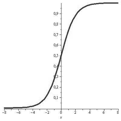
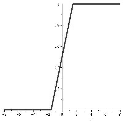
Figure 1: The plots of $\sigma_{\ell}$ (left) and $\sigma_{R}$ (right), i.e., the logistic and the ramp sigmoidal functions.

Such kind of sigmoidal functions are the most used in the applications by means of neural networks, since their smoothness make them very suitable for the implementation of learning algorithms, such as the well-known back-propagation algorithm, see e.g. [51, 8, 35, 36, 38, 43, 44, 49].

Assumptions $(\Sigma 1)$, $(\Sigma 2)$, and $(\Sigma 3)$ required in order to apply the present theory, are satisfied in both the above cases. In particular, we can observe that both $\sigma_{\ell}$ and $\sigma_{h}$ have an exponential decay to zero as $x\to-\infty$, then condition $(\Sigma 3)$ is satisfied for every $\alpha>0$, see e.g., [26].

The above exponential decay of $\sigma_{\ell}$ and $\sigma_{h}$, it is then inherited from the corresponding univariate and multivariate density functions $\phi_{\sigma_{\ell}}(x)$ (see Fig. 2, left), $\phi_{\sigma_{h}}(x)$, and $\Psi_{\sigma_{\ell}}(\underline{x})$ (see Fig. 3, left), $\Psi_{\sigma_{h}}(\underline{x})$, for $|x|\to+\infty$, and $\|\underline{x}\|_{2}\to+\infty$, respectively.

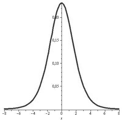
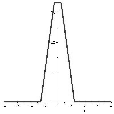
Figure 2: The plots of the $\phi_{\sigma_{\ell}}$ (left) and $\phi_{\sigma_{R}}$ (right).

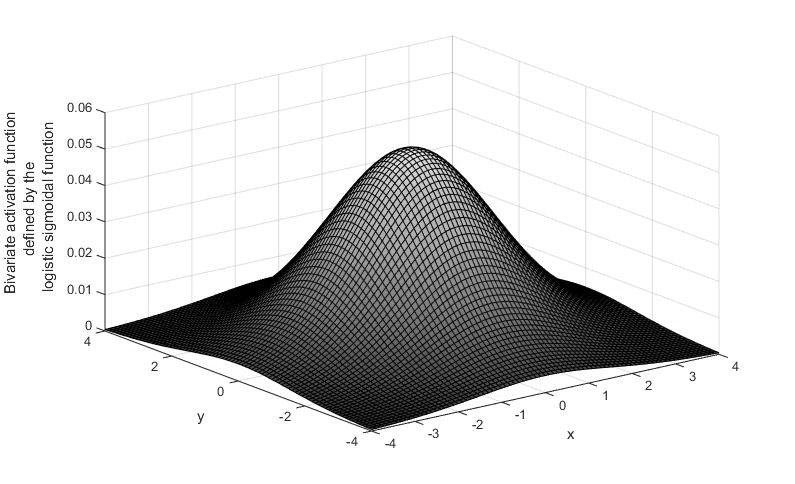
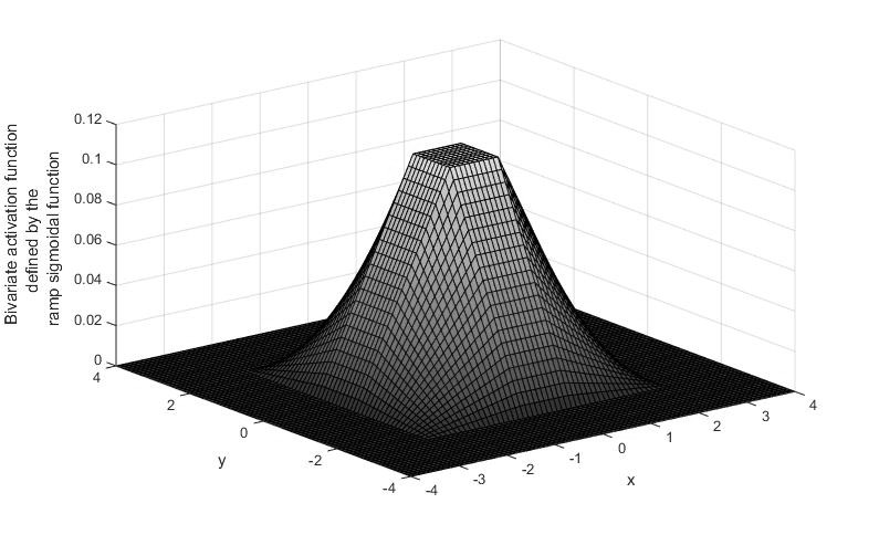
Figure 3: The plots of the bivariate functions $\Psi_{\sigma_{\ell}}$ (left) and $\Psi_{\sigma_{R}}$ (right).

Further, since the above theory still holds in case of not necessarily smooth sigmoidal functions, we also provide examples of such functions.

An example of non-smooth, but continuous sigmoidal activation function is given by the well-known ramp function $\sigma_{R}$ (see e.g. [19, 25] and Fig. 1, right) defined by:

$$\sigma_{R}(x)\ :=\ \left\{\begin{array}[]{l}0,\hskip 79.6678ptx<-3/2,\\ x/3+(1/2),\hskip 25.6073pt-3/2\leq x\leq 3/2,\\ 1,\hskip 79.6678ptx>3/2.\end{array}\right.$$

In addition, it is easy to see that $(\Sigma 3)$ is satisfied for every $\alpha>0$, and the corresponding $\phi_{\sigma_{R}}$, $\Psi_{\sigma_{R}}$ (see Fig. 2 right and Fig. 3 right, respectively) have compact support.

The above sigmoidal functions can be used in order to obtain the modular convergence for the operators $K^{(M)}_{n}$ in some well-known examples of Orlicz spaces.

For instance, we can consider the Orlicz spaces generated by the convex $\varphi$-function $\varphi(u):=u^{p}$, $u\geq 0$, $1\leq p<+\infty$, i.e., the well-known $L^{p}({\cal R})$ spaces (see e.g., [13]). If we consider the non-negative functions belonging to $L^{p}({\cal R})$ we define as above the space $L^{p}_{+}({\cal R})$. Further, we can also observe that, the above $\varphi$-function satisfies the $\Delta_{2}$-condition, then the modular convergence coincides with the norm-convergence.

Here, it turns out that $I^{\varphi}[f]=\|f\|_{p}^{p}$, and Theorem 3.3 becomes:

Corollary 4.1.

For any $f\in L^{p}_{+}({\cal R})$, $1\leq p<+\infty$, we have:

$$\lim_{n\to+\infty}\|K^{(M)}_{n}(f,\cdot)-f(\cdot)\|_{p}\ =\ 0,$$

where $K^{(M)}_{n}$ can be considered generated by all the above mentioned examples of sigmoidal functions.

Other useful examples of Orlicz spaces are the interpolation spaces $L^{\alpha}\log^{\beta}L({\cal R})$ (also known as the Zygmund spaces). Such spaces, can be generated by the $\varphi$-functions $\varphi_{\alpha,\beta}(u):=u^{\alpha}\log^{\beta}(u+e)$, for $\alpha\geq 1$, $\beta>0$, $u\geq 0$. Note that, also $\varphi_{\alpha,\beta}$ satisfies the $\Delta_{2}$-condition, then modular convergence and norm-convergence are equivalent. The convex modular functional corresponding to $\varphi_{\alpha,\beta}$ are:

$$I^{\varphi_{\alpha,\beta}}[f]:=\int_{\cal R}|f(\underline{x})|^{\alpha}\log^{\beta}(e+|f(\underline{x})|)\ d\underline{x},\ \hskip 14.22636pt(f\in M({\cal R})).$$

Obviously, if we consider the non-negative (a.e.) functions belonging to $L^{\alpha}\log^{\beta}L({\cal R})$, we can define the space $L^{\alpha}_{+}\log^{\beta}L({\cal R})$.

Finally, as last examples, we recall the exponential spaces (and the corresponding space of the a.e. non-negative functions) generated by $\varphi_{\gamma}(u)=e^{u^{\gamma}}-1$, for $\gamma>0$, $u\geq 0$. In this latter case, the $\Delta_{2}$-condition is not satisfied, then the norm convergence it turns out strictly stronger than the modular one. The modular functional corresponding to $\varphi_{\gamma}$ is:

$$I^{\varphi_{\gamma}}[f]:=\int_{\cal R}(e^{|f(\underline{x})|^{\gamma}}-1)\ d\underline{x},\ \hskip 14.22636pt(f\in M({\cal R})).$$

In both the last two examples, the modular inequality of Theorem 3.2 and the modular convergence of Theorem 3.3 hold, and an analogous of Corollary 4.1 can be stated.

For further examples of Orlicz spaces and sigmoidal functions, see e.g., [15, 13, 22, 50, 52].

5 Applications to real world cases

In this section, we provide some applications of the above results in some concrete cases.

We begin considering a real world case involving one-dimensional data in order to show the modeling capabilities of the above neural network operators.

In the table of Fig. 4, it has been reported the data provided by the official dataset of the website www.tuttitalia.it concerning the trend of the Italian, Foreign, and Total population living in Perugia (Italy) from 2004 to 2017.

Figure 4: The trend of the Italian, Foreign, and Total population living in Perugia (Italy) from 2004 to 2017. The entries of the above table represent the average population for each considered year. The above data have been considered from the official dataset of the website www.tuttitalia.it.

The entries of the above table represent the average population for each considered year.

The above data have been modeled by the max-product neural network operators $K^{(M)}_{n}(f,\cdot)$ in the one-dimensional case, and based upon the density function $\phi_{\sigma_{\ell}}$ generated by the logistic function $\sigma_{\ell}$.

More precisely, the above data have been modeled by the operators $K^{(M)}_{13}(f,\cdot)$ (i.e., with $n=13$) on the interval $[a,b]=[0,1]$. Here, the years from $2004$ to $2017$ have been mapped on the nodes $k/n$, with $k=0,1,\dots,n$, $n=13$; the averages

$$n\,\int_{k/n}^{(k+1)/n}f(u)\,du,$$

have been replaced with the data of the first, the second and the third column of the table in Fig. 4, respectively. The plots of the described neural network models have been given in Fig. 5.

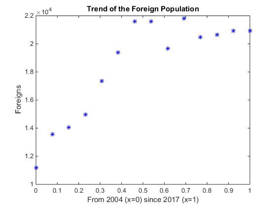
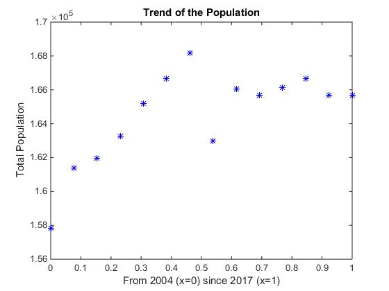
Figure 5: The modeled trends of the Italian, Foreign, and Total population living in Perugia (Italy) from 2004 to 2017 modeled by the max-product neural network operators $K^{(M)}_{13}(f,\cdot)$.

We stress that, the above example has been given with the main purpose to show that the max-product neural network operators can be used also to model data arising from real world problems and not only for the theoretical approximation of mathematical functions defined by a certain analytical expression.

Applications in case of phenomenon involving multivariate data, can be given considering the case of image reconstruction and enhancement. This subject is very related to Kantorovich-type operators (see, e.g., [6, 7]) since they revealed to be suitable in case of reconstruction of not necessarily continuous data (see, e.g., Corollary 4.1) and in general, images are the most common examples of multivariate discontinuous functions. Indeed, any static gray scale image presents at the edges of the figures, jumps of gray levels in the gray scale, and from the mathematical point of view, these can be modeled by means of discontinuities.

For instance, using, e.g., the bi-variate version of the above max-product neural network operators we can reconstruct images on a certain domain starting from a discrete set of mean values only.

More precisely, using a model of the data similar to those used in the one-dimensional case, and knowing that by the above operators we can approximate data on a continuous domain, we can reconstruct any given image on the same nodes of the original one, or at a grid of nodes of higher dimension, in fact obtaining a reconstructed image with higher resolution with respect to the original one.

For instance, in Fig. 6 we have a vascular CT image (computer tomography) representing an aneurysm of the abdominal aorta artery.

Figure 6: A portion of the abdominal aorta artery depicting an aneurysm of resolution $60\times 60$ pixels (source: Santa Maria della Misericordia Hospital of Perugia - Italy).

The image in Fig. 6 has a low resolution ($60\times 60$ pixels) and the edges of the vessel are not clearly detectable, then from the diagnostic point of view, the image have a low utility.

First of all, a mere reconstruction of the above vascular image can be given, e.g., by the bi-variate max-product neural network operator $K^{(M)}_{n}$ based upon the bi-variate density function $\Psi_{\sigma_{\ell}}$ generated by the logistic function $\sigma_{\ell}$, with various $n$ (see Fig. 7).

Figure 7: The reconstruction of the original image in Fig. 6 by the max-product operators $K^{(M)}_{n}$ with $n=5$ (on the left) and $n=10$ (on the right).

Finally, in Fig. 8 are shown the reconstruction of the original image of Fig. 6 by the max-product operators $K^{(M)}_{n}$ with $n=5$ and $n=20$, respectively obtained by a double resolution, i.e., $120\times 120$ pixels, with respect to the original one. In this sense, the images in Fig. 8 have been enhanced with respect to that of Fig. 6.

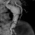
Figure 8: The reconstruction of the original image in Fig. 6 by the max-product operators $K^{(M)}_{n}$ with $n=5$ (on the left) and $n=20$ (on the right). Note that, the above reconstructions have been given by a double resolution (i.e., $120\times 120$ pixels) with respect to the original image.

Indeed, we can observe that here the contours and the edges of the vessels are more defined with respect to the original one. Hence, NN operators open also an application field in image reconstruction and enhancement.

Conflict of interest The authors declare that they have no conflict of interest.

Ethical statement Ethical approval was waived considering that the CT images analyzed were anonymized and the results did not influence any clinical judgment.

References

- [1] A. Adler, R. Guardo, A Neural Network Image Reconstruction Technique for Electrical Impedance Tomography, IEEE Trans. on Medical Imaging, 13 (4), (1994) 594-600.
- [2] L. Angeloni, D. Costarelli, G. Vinti, A characterization of the convergence in variation for the generalized sampling series, Annales Academiae Scientiarum Fennicae Mathematica, 43 (2018) 755-767.
- [3] L. Angeloni, G. Vinti, Convergence and rate of approximation for linear integral operators in -spaces in multidimensional setting, Journal of Mathematical Analysis and Applications, 349 (2009), 317-334.
- [4] L. Angeloni, G. Vinti, Approximation with respect to Goffman-Serrin variation by means of non-convolution type integral operators, Numerical Functional Analysis and Optimization, 31 (2010) 519-548.
- [5] L. Angeloni, G. Vinti, Convergence and rate of approximation in BV for a class of Mellin integral operators, Atti Accad. Naz. Lincei Cl. Sci. Fis. Mat. Natur. Rend. Lincei, (9), Mat. Appl., 25 (2014) 217-232.
- [6] F. Asdrubali, G. Baldinelli, F. Bianchi, D. Costarelli, A. Rotili, M. Seracini, G. Vinti, Detection of thermal bridges from thermographic images by means of image processing approximation algorithms, Applied Mathematics and Computation, 317 (2018) 160-171.
- [7] F. Asdrubali, G. Baldinelli, F. Bianchi, D. Costarelli, L. Evangelisti, A. Rotili, M. Seracini, G. Vinti, A model for the improvement of thermal bridges quantitative assessment by infrared thermography, Applied Energy, 211 (2018) 854-864.
- [8] K. R. Ball, C. Grant, W. R. Mundy, T. J. Shafera, A multivariate extension of mutual information for growing neural networks, Neural Networks, 95 (2017) 29-43.
- [9] C. Bardaro, H. Karsli, G. Vinti, Nonlinear integral operators with homogeneous kernels: Pointwise approximation theorems, Applicable Analysis, 90 (3-4) (2011), 463-474.
- [10] C. Bardaro, J. Musielak, G. Vinti, Nonlinear Integral Operators and Applications, New York, Berlin: De Gruyter Series in Nonlinear Analysis and Applications 9, 2003.
- [11] B. Bartoccini, D. Costarelli, G. Vinti, Extension of saturation theorems for the sampling Kantorovich operators, in print in: Complex Analysis and Operator Theory (2018) DOI: 10.1007/s11785-018-0852-z.
- [12] B. Bede, L. Coroianu, S.G. Gal, Approximation By Max-Product Type Operators, Springer International Publishing, 2016, DOI: 10.1007/978-3-319-34189-7.
- [13] A. Boccuto, D. Candeloro, A. R. Sambucini, spaces in vector lattices and applications, Math. Slov., 67 (6), (2017) 1409-1426, DOI: 10.1515/ms-2017-0060.
- [14] A. Bono-Nuez, C. Bernal-Ruíz, B. Martín-del-Brío, F. J. Pérez-Cebolla, A. Martínez-Iturbe, Recipient size estimation for induction heating home appliances based on artificial neural networks, Neural Computing and Applications, 28 (11) (2017) 3197-3207.
- [15] D. Candeloro, A. R. Sambucini, Filter convergence and decompositions for vector lattice-valued measures, Mediterranean J. Math., 12 (3) (2015) 621-637, DOI: 10.1007/s00009-014-0431-0 .
- [16] F. Cao, Z. Chen, The approximation operators with sigmoidal functions, Comput. Math. Appl. 58 (4) (2009) 758-765.
- [17] F. Cao, Z. Chen, The construction and approximation of a class of neural networks operators with ramp functions, J. Comput. Anal. Appl. 14 (1) (2012) 101-112.
- [18] F. Cao, B. Liu, D.S. Park, Image classification based on effective extreme learning machine, Neurocomputing 102 (2013), 90-97.
- [19] G. H. L. Cheang, Approximation with neural networks activated by ramp sigmoids, J. Approx. Theory 162 (2010) 1450-1465.
- [20] L. Coroianu, S.G. Gal, Saturation and inverse results for the Bernstein max-product operator, Period. Math. Hungar 69 (2014), 126-133.
- [21] L. Coroianu, S.G. Gal, -approximation by truncated max-product sampling operators of Kantorovich-type based on Fejer kernel, Journal of Integral Equations and Applications, 29 (2) (2017), 349-364.
- [22] D. Costarelli, A.M. Minotti, G. Vinti, Approximation of discontinuous signals by sampling Kantorovich series, Journal of Mathematical Analysis and Applications, 450 (2) (2017) 1083-1103.
- [23] D. Costarelli, A.R. Sambucini, Approximation results in Orlicz spaces for sequences of Kantorovich max-product neural network operators, Results in Mathematics, 73 (1) (2018) DOI: 10.1007/s00025-018-0799-4.
- [24] D. Costarelli, R. Spigler, How sharp is the Jensen inequality?, Journal of Inequalities and Applications, 2015:69 (2015) 1-10.
- [25] D. Costarelli, R. Spigler, Solving numerically nonlinear systems of balance laws by multivariate sigmoidal functions approximation, Computational and Applied Mathematics, 37 (1) (2018) 99-133.
- [26] D. Costarelli, G. Vinti, Approximation by max-product neural network operators of Kantorovich type, Results in Mathematics, 69 (3) (2016), 505-519.
- [27] D. Costarelli, G. Vinti, Max-product neural network and quasi-interpolation operators activated by sigmoidal functions, Journal of Approximation Theory, 209 (2016), 1-22.
- [28] D. Costarelli, G. Vinti, Pointwise and uniform approximation by multivariate neural network operators of the max-product type, Neural Networks, 81 (2016) 81-90.
- [29] D. Costarelli, G. Vinti, Saturation classes for max-product neural network operators activated by sigmoidal functions, Results in Mathematics, 72 (3) (2017) 1555-1569.
- [30] D. Costarelli, G. Vinti, Convergence for a family of neural network operators in Orlicz spaces, Mathematische Nachrichten, 290 (2-3) (2017) 226-235.
- [31] D. Costarelli, G. Vinti, Convergence results for a family of Kantorovich max-product neural network operators in a multivariate setting, Mathematica Slovaca, 67 (6) (2017), 1469-1480.
- [32] D. Costarelli, G. Vinti, Estimates for the neural network operators of the max-product type with continuous and p-integrable functions, Results in Mathematics, 73 (1) (2018) DOI: 10.1007/s00025-018-0790-0.
- [33] D. Costarelli, G. Vinti, An inverse result of approximation by sampling Kantorovich series, in print in: Proceedings of the Edinburgh Mathematical Society (2018) DOI:10.1017/S0013091518000342.
- [34] M. Egmont-Petersena, D. de Ridderb, H. Handels, Image processing with neural networks-a review, Pattern Recognition, 35 (2002) 2279-2301.
- [35] G. Gnecco, A comparison between fixed-basis and variable-basis schemes for function approximation and functional optimization, J. Appl. Math., (2012) ID 806945, 17 pp.
- [36] G. Gnecco, M. Sanguineti, On a Variational Norm Tailored to Variable-Basis Approximation Schemes, IEEE Trans. Inform. Theory, 57 (2011) 549-558.
- [37] A.T.C. Goh, Back-propagation neural networks for modeling complex systems, Artificial Intelligence in Engineering, 9 (1995), 143-151.
- [38] D. Gotleyb, G. Lo Sciuto, C. Napoli, R. Shikler, E. Tramontana, M. Wozniak, Characterization and Modeling of Organic Solar Cells by Using Radial Basis Neural Networks, in: Artificial Intelligence and Soft Computing, (2016) 91-103, DOI: .
- [39] N.J. Guliyev, V.E. Ismailov, On the approximation by single hidden layer feedforward neural networks with fixed weights, Neural Networks 98 (2018) 296-304
- [40] N.J. Guliyev, V.E. Ismailov, Approximation capability of two hidden layer feedforward neural networks with fixed weights, Neurocomputing 316 (2018) 262-269.
- [41] A. Iliev, N. Kyurkchiev, S. Markov, On the approximation of the cut and step functions by logistic and Gompertz functions, BIOMATH, 4 (2), (2015) 1510101.
- [42] P.C. Kainen, V. Kurkova, M. Sanguineti, Complexity of Gaussian-radial-basis networks approximating smooth functions, J. Complexity, 25 (1) (2009) 63-74.
- [43] G. Lai, Z. Liu, Y. Zhang, C. L. Philip Chen, Adaptive position/attitude tracking control of aerial robot with unknown inertial matrix based on a new robust neural identifier, IEEE Trans. Neural Netw. and Learning Systems, 27 (1) (2016), 18-31.
- [44] P. Liu, J. Wang, Z. Zeng, Multistability of delayed recurrent neural networks with Mexican hat activation functions, Neural Computation, 29 (2) (2017), 423-457.
- [45] D.J. Livingstone, Artificial Neural Networks: Methods and Applications (Methods in Molecular Biology), Humana Press, 2008.
- [46] V. Maiorov, Approximation by neural networks and learning theory, J. Complexity 22 (1) (2006) 102-117.
- [47] J. Musielak, Orlicz Spaces and Modular Spaces, Springer-Verlag, Lecture Notes in Math. 1034, 1983.
- [48] J. Musielak, W. Orlicz, On modular spaces, Studia Math. 28 (1959), 49-65.
- [49] J.J. Olivera, Global exponential stability of nonautonomous neural network models with unbounded delays, Neural Networks, 96 (2017), 71-79.
- [50] B. Rister, D. L. Rubin, Piecewise convexity of artificial neural networks, Neural Networks, 94 (2017) 34-45.
- [51] A. Sahoo, H. Xu, S. Jagannathan, Adaptive neural network-based event-triggered control of single-input single-output nonlinear discrete-time systems, IEEE Trans. Neural Netw. and Learning Systems, 27 (1) (2016), 151-164.
- [52] G. Stamov, I. Stamova, Impulsive fractional-order neural networks with time-varying delays: almost periodic solutions, Neural Computing and Applications, 28 (11) (2017) 3307-3316.