Location-free Spectrum Cartography

Abstract

Spectrum cartography constructs maps of metrics such as channel gain or received signal power across a geographic area of interest using spatially distributed sensor measurements. Applications of these maps include network planning, interference coordination, power control, localization, and cognitive radios to name a few. Since existing spectrum cartography techniques require accurate estimates of the sensor locations, their performance is drastically impaired by multipath affecting the positioning pilot signals, as occurs in indoor or dense urban scenarios. To overcome such a limitation, this paper introduces a novel paradigm for spectrum cartography, where estimation of spectral maps relies on features of these positioning signals rather than on location estimates. Specific learning algorithms are built upon this approach and offer a markedly improved estimation performance than existing approaches relying on localization, as demonstrated by simulation studies in indoor scenarios.

I Introduction

Spectrum cartography constructs maps of a certain channel metric, such as received signal power, power spectral density (PSD), or channel gain over a geographical area of interest by relying on measurements collected by radio frequency (RF) sensors [2, 3, 4]. The obtained maps are of utmost interest in a number of tasks in wireless communication networks, such as network planning, interference coordination, power control, and dynamic spectrum access [5, 6, 7]. For instance, power maps can be useful in network planning since the former indicate areas of weak coverage, thus suggesting locations where new base stations must be deployed. Since PSD maps characterize the distribution of the RF signal power per channel over space, they can play a major role in increasing frequency reuse to mitigate interference. These maps may also be of interest to speed up hand-off in cellular networks since they enable mobile users to determine the power of all channels at a given location without having to spend time measuring it. Additional use cases may include cognitive radios, where secondary users aim at exploiting underutilized spectrum resources in the space-frequency-time domain, or source localization, where the locations of certain transmitters may be estimated by inspecting a map [3].

Existing methods for mapping RF power apply spatial interpolation or regression techniques to power measurements collected by spatially distributed sensors. Some of these methods include kriging [8, 2, 9], orthogonal matchning pursuit [4], matrix completion [10], dictionary learning [11, 12], sparse Bayesian learning [13], or kernel-based learning [14, 15]. Since these works can only map power distribution across space but not across frequency, different schemes have been devised to construct PSD maps, for instance by exploiting the sparsity of power distributions over space and frequency with a basis expansion model [3, 16] or by leveraging the framework of kernel-based learning [5]. Rather than mapping power, other families of methods construct channel-gain maps using Kriged Kalman filtering [17], non-parametric regression in reproducing kernel Hilbert spaces (RKHSs) [18], low rank and sparsity [19], or hidden Markov random fields [20].

All the aforementioned schemes require accurate knowledge of the sensor locations. For this reason, they will be collectively referred to as location-based (LocB) cartography. However, location is seldom known in practice and therefore must be estimated from features such as the received signal strength, the time (difference) of arrival (T(D)oA), or the direction of arrival (DoA) of positioning pilot signals transmitted by satellites (e.g. in GPS) or terrestrial base stations (e.g. in LTE or WiFi [21]) [22, 23]. Unfortunately, accurate location estimates are often not available in practice due to propagation phenomena affecting those pilot signals such as multipath, which limits the applicability of existing cartography techniques, especially in indoor and dense urban scenarios. To see the intuition behind this observation, Figs. 1a and 1b respectively show the $x$ and $y$ coordinates of the location estimates obtained by applying a state-of-the-art localization algorithm to TDoA measurements of 5 pilot signals received in free space (details of the specific simulation setting can be found in Sec. V). On the other hand, Figs. 1c and 1d depict the same estimates but in an indoor propagation scenario. As observed, the estimates in the second case are neither accurate nor smooth across space, which precludes any reasonable estimate of a spectrum map based on them.

To counteract this difficulty, there are three main types of indoor positioning systems [24]: (i) Those based on ultra-wideband (UWB) [25, 26, 27], which require a dedicated infrastructure and relatively high costs, e.g. synchronized anchor nodes in the area where the map has to be constructed. Therefore, localization cannot be carried out in an area where such hardware is not present. (ii) Other indoor positioning systems are based on fingerprinting [28, 29, 24], which involves a manual collection and storage of a dataset. This dataset may comprise the measured power of multiple beacons at a set of known locations. Note that this process is time consuming and typically expensive because a human or robot should physically go through several known locations to take measurements. Furthermore, if there are significant changes in the propagation environment, these methods would require the acquisition of a new dataset. (iii) There exist other indoor positioning systems that combine UWB or fingerprinting with ultrasound [30] or RFID [31]. Thus, they inherit the limitations of (i) and (ii) and require furthermore special sensors and/or line-of-sight propagation conditions. To sum up, all existing cartography schemes require accurate location information, which is not available in dense multipath and indoor scenarios when there are no special localization infrastructure or fingerprinting datasets.

The main contribution of this paper is to address this limitation by proposing the framework of location-free (LocF) cartography. The key observation is that inaccurate location estimates introduce significant errors in spectrum map estimation. To bypass this limitation, the proposed approach obtains spectrum maps indexed directly by (or as a function of) features of the received pilot signals. Although many algorithms can be devised within this framework, the present paper develops an algorithm based on kernel-based learning for the sake of exposition. This is not only because of the simplicity, flexibility, and good performance of kernel-based estimators, but also because they have well-documented merits in spectrum cartography [16, 5]. Similarly, the discussion focuses on constructing power maps, but the proposed paradigm carries over to other metrics such as PSD. Remarkably, as a byproduct of skipping the localization step, the resulting cartography algorithm is typically computationally less expensive than its LocB counterparts and does not require additional localization infrastructure or the costly creation of fingerprinting datasets. The second main contribution is a design of pilot signal features tailored to multipath environments. The third contribution is a special technique to accommodate scenarios where a sensor can only extract a subset of those features due to low signal-to-noise ratio (SNR). Finally, the proposed LocF cartography scheme is studied through Monte Carlo simulations in realistic propagation environments. As expected, the proposed scheme outperforms LocB cartography in multipath scenarios, but traditional LocB approaches are still preferable when accurate location estimates are available.

The rest of this paper is structured as follows: Sec. II describes the system model, states the problem, and reviews LocB cartography. Sec. III introduces LocF cartography along with the proposed map estimation algorithm, whereas Sec. IV deals with feature design. Numerical tests are presented in Sec. V, and conclusions in Sec. VI.

Notation: Scalars are denoted by lowercase letters. Bold uppercase (lowercase) letters denote matrices (column vectors), $\bm{I}_{N}$ is the $N\times N$ identity matrix and $\bm{1}$ is the vector of all ones of appropriate dimension. The symbol ${{\color[rgb]{0,0,0}\jmath}}:=\sqrt{-1}$ is the imaginary unit, ${(\cdot)^{*}}$ stands for the complex conjugate, while $\ast$ denotes convolution. Furthermore, operators $(\cdot)^{\top}$ and $||\cdot||_{F}$ represent transposition and the Frobenius norm, respectively.

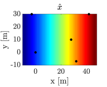
(a)

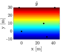
(b)

(c)

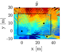
(d)

Figure 1: Estimation of spatial coordinates using TDoA: (a)-(b) in free space, (c)-(d) indoor where the solid black lines represent the walls of the building; the black dots represent the locations of the anchor base stations. The color of each pixel represents the value of the estimated location coordinate at each point in the $150\times 150$ grid area. Because location estimates in (a)-(b) coincide with the true locations, they can act as colorbars to the estimates in (c)-(d).

II Problem Formulation and LocB Cartography

This section formulates the general spectrum cartography problem and reviews the basics of LocB cartography.

F The goal is to determine the power $p(\bm{x})$ of a certain channel, termed channel-to-map (C2M), at every location $\bm{x}\in\mathcal{X}$ of a geographical region of interest $\mathcal{X}\subset\mathbb{R}^{d}$, with $d=2$ or $3$. For example, this C2M can be an uplink or downlink channel of a cellular network as well as a radio or TV broadcasting channel. To this end, a collection of sensors gather $N$ measurements at locations $\{\bm{x}_{n}\}_{n=1}^{N}\subset\mathcal{X}$ not necessarily known. The noisy measurement of the power $p(\bm{x}_{n})$ at location $\bm{x}_{n}$ will be represented as $\tilde{p}_{n}$. Since the sensors collect measurements at multiple locations in $\mathcal{X}$, the number of measurements may be significantly greater than the number of sensors.

In LocB cartography [2, 9, 4, 11, 12, 10, 13, 15, 3, 16, 5, 18, 19, 20], a fusion center is ideally given pairs $\{(\bm{x}_{n},\tilde{p}_{n})\}_{n=1}^{N}$, which include the exact sensor locations $\{\bm{x}_{n}\}_{n=1}^{N}$, and obtains a function estimate $\hat{p}(\bm{x})$ that provides the power of the C2M at any query location $\bm{x}\in\mathcal{X}$. With this function, a node at location $\bm{x}$ can determine the power of the C2M if it knows $\bm{x}$. In practice, however, location is typically unknown and hence the sensor at the $n$-th measurement point must estimate $\bm{x}_{n}$ by relying on pilot signals $\{{{\color[rgb]{0,0,0}y}}_{{{\color[rgb]{0,0,0}l}},n}[k]\}_{{{\color[rgb]{0,0,0}l}}=1}^{{\color[rgb]{0,0,0}L}}$, where ${{\color[rgb]{0,0,0}y}}_{{{\color[rgb]{0,0,0}l}},n}[k]$ denotes the $k$-th sample of the pilot signal transmitted by the ${{\color[rgb]{0,0,0}l}}$-th base station and received at the $n$-th measurement point. For convenience, form the ${{\color[rgb]{0,0,0}L}}\times K$ matrix ${\color[rgb]{0,0,0}\bm{Y}}_{n}$ whose $({{\color[rgb]{0,0,0}l}},k)$-th entry is ${{\color[rgb]{0,0,0}y}}_{{{\color[rgb]{0,0,0}l}},n}[k]$. Note that these pilot signals are generally transmitted through a separate channel, not necessarily the C2M. However, both channels may coincide, as it occurs in certain cellular communication standards.

From ${\color[rgb]{0,0,0}\bm{Y}}_{n}$, the sensor at the $n$-th measurement point obtains the estimate ${\hat{\bm{x}}}_{n}:={\hat{\bm{x}}}({\color[rgb]{0,0,0}\bm{Y}}_{n})$ of $\bm{x}_{n}$ by means of some localization algorithm [22, 23]. A fusion center then uses $\{({\hat{\bm{x}}}_{n},\tilde{p}_{n})\}_{n=1}^{N}$ to obtain an estimate $\hat{p}(\bm{x})$ of the function $p(\bm{x})$. Therefore, if the location estimates $\{{\hat{\bm{x}}}_{n}\}_{n=1}^{N}$ are noisy, so will be $\hat{p}(\bm{x})$. If a node at an unknown query location wishes to determine the power of the C2M, it will use the pilot signals ${\color[rgb]{0,0,0}\bm{Y}}$ to obtain an estimate ${\hat{\bm{x}}}:={\hat{\bm{x}}}({\color[rgb]{0,0,0}\bm{Y}})$ of its location and will evaluate the map estimate as $\hat{p}({\hat{\bm{x}}})$. In this case, ${\color[rgb]{0,0,0}\bm{Y}}$ is a matrix whose $({{\color[rgb]{0,0,0}l}},k)$-th entry is given by the $k$-th sample of the ${{\color[rgb]{0,0,0}l}}$-th pilot signal ${{\color[rgb]{0,0,0}y}}_{{{\color[rgb]{0,0,0}l}}}[k]$ at the query location. Thus, such an estimation has two sources of error: first, the location estimation error in ${\hat{\bm{x}}}$ and, second, the map estimation error in $\hat{p}(\bm{x})$.

Remark 1

One may argue that a node can determine the power of the C2M at its location more efficiently by measuring it rather than by receiving the pilot signals, applying a localization algorithm, and evaluating the map. Whereas this may be the case for a single C2M, if the aim is to determine the PSD, the power of many C2Ms, or the impulse response, then the associated measurement time may be prohibitive, which favors the adoption of spectrum cartography approaches.

III Location-Free Cartography

This section proposes LocF cartography, which bypasses the localization step involved in all existing cartography approaches. To this end, the LocF cartography problem is formulated as a function estimation task in Sec. III-A and solved via kernel-based learning in Sec. III-B.

III-A Map Estimate as a Function Composition

As detailed in the previous section, existing spectrum cartography techniques are heavily impaired by localization errors since the maps they construct are functions of noisy location estimates. The main idea of the proposed framework is to bypass such a dependence.

To this end, it is worth interpreting LocB cartography from a more abstract perspective. As detailed in Sec. II, the LocB map estimate is of the form $\hat{p}({\hat{\bm{x}}})$ with ${\hat{\bm{x}}}:={\hat{\bm{x}}}({\color[rgb]{0,0,0}\bm{Y}})$ denoting the output of the selected localization algorithm when the pilot signals are given by ${\color[rgb]{0,0,0}\bm{Y}}\in\mathcal{Y}$. Thus, this estimate can be seen as a function of ${\color[rgb]{0,0,0}\bm{Y}}$, i.e. ${\color[rgb]{0,0,0}\hat{p}_{{\color[rgb]{0,0,0}\bm{Y}}}}({\color[rgb]{0,0,0}\bm{Y}}):=\hat{p}({\hat{\bm{x}}}({\color[rgb]{0,0,0}\bm{Y}}))$, which can be expressed schematically as:

$$\begin{aligned} &\mathcal{Y}&\overset{\hat{\bm{x}}}{\xrightarrow{\hskip 19.91684pt}}&\quad\mathcal{X}&\overset{\hat{p}}{\xrightarrow{\hskip 19.91684pt}}&\quad\mathbb{R}\\ &{\color[rgb]{0,0,0}\bm{Y}}&\xrightarrow{\hskip 19.91684pt}&\quad\hat{\bm{x}}({\color[rgb]{0,0,0}\bm{Y}})&\xrightarrow{\hskip 19.91684pt}&\quad\hat{p}({\hat{\bm{x}}}({\color[rgb]{0,0,0}\bm{Y}})).\end{aligned}$$ (1)

As mentioned in Sec. II, existing (LocB) cartography approaches obtain an estimate $\hat{p}$ of $p$ using the data $\{({\hat{\bm{x}}}({\color[rgb]{0,0,0}\bm{Y}}_{n}),\tilde{p}_{n})\}_{n=1}^{N}$ for instance by searching for a function in an RKHS [14, 5, 15]. When ${\hat{\bm{x}}}({\color[rgb]{0,0,0}\bm{Y}})$ is a reasonable estimate of the location $\bm{x}$ at which ${\color[rgb]{0,0,0}\bm{Y}}$ has been observed, such a LocB approach works well. However, due to multipath propagation effects impacting the pilot signals in ${\color[rgb]{0,0,0}\bm{Y}}$, ${\hat{\bm{x}}}({\color[rgb]{0,0,0}\bm{Y}})$ may be very different from $\bm{x}$, which drastically hinders the estimation of $p$. Thus, in those cases where the location estimates $\{{\hat{\bm{x}}}({\color[rgb]{0,0,0}\bm{Y}}_{n})\}_{n=1}^{N}$ are noisy, the resulting estimate $\hat{p}$, and consequently ${\color[rgb]{0,0,0}\hat{p}_{{\color[rgb]{0,0,0}\bm{Y}}}}$, will be correspondingly noisy.

Since the source of such an error is the dependency of ${\color[rgb]{0,0,0}\hat{p}_{{\color[rgb]{0,0,0}\bm{Y}}}}({\color[rgb]{0,0,0}\bm{Y}})=\hat{p}({\hat{\bm{x}}}({\color[rgb]{0,0,0}\bm{Y}}))$ on the estimated location ${\hat{\bm{x}}}({\color[rgb]{0,0,0}\bm{Y}})$, one could think of bypassing this dependence by directly estimating ${\color[rgb]{0,0,0}\hat{p}_{{\color[rgb]{0,0,0}\bm{Y}}}}$ as a general function of ${\color[rgb]{0,0,0}\bm{Y}}$:

$$\begin{aligned} &\mathcal{Y}&\overset{{\color[rgb]{0,0,0}\hat{p}_{{\color[rgb]{0,0,0}\bm{Y}}}}}{\xrightarrow{\hskip 19.91684pt}}&\quad\mathbb{R}\\ &{\color[rgb]{0,0,0}\bm{Y}}&\xrightarrow{\hskip 19.91684pt}&\quad{\color[rgb]{0,0,0}\hat{p}_{{\color[rgb]{0,0,0}\bm{Y}}}}({\color[rgb]{0,0,0}\bm{Y}}).\end{aligned}$$ (2)

When pursuing an estimate of this general form, ${\color[rgb]{0,0,0}\hat{p}_{{\color[rgb]{0,0,0}\bm{Y}}}}({\color[rgb]{0,0,0}\bm{Y}})$ would not be confined to depend on ${\color[rgb]{0,0,0}\bm{Y}}$ only through the estimated location. However, finding such an estimate given $\{({\color[rgb]{0,0,0}\bm{Y}}_{n},\tilde{p}_{n})\}_{n=1}^{N}$ by searching over a generic class of functions such as an RKHS would be extremely challenging due the so-called curse of dimensionality [32, 33]. To intuitively understand this phenomenon, note that the number of input variables of function ${\color[rgb]{0,0,0}\hat{p}_{{\color[rgb]{0,0,0}\bm{Y}}}}({\color[rgb]{0,0,0}\bm{Y}})$ is ${{\color[rgb]{0,0,0}L}}K$, typically in the order of hundreds or thousands. Since learning a multivariate function up to a reasonable accuracy generally requires that the number of data points be several orders of magnitude larger than the number of input variables, this approach would need $N$ to be significantly larger than ${{\color[rgb]{0,0,0}L}}K$, and therefore prohibitively large.

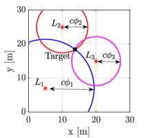
(a)

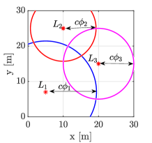
(b)

Figure 2: Multi-lateration using ToA measurements with circles as possible sensor locations: (a) consistent ToA with the sought sensor location being the intersection of the circles (black square) and (b) inconsistent ToA measurements. The red stars represent the locations of the anchor base stations.

To summarize, the structure imposed by (LABEL:eq:locasedDirect) is too generic, whereas the one imposed by (LABEL:eq:locasedComp) is too restrictive. To attain a sweet spot in this trade-off, it is worth decomposing ${\hat{\bm{x}}}({\color[rgb]{0,0,0}\bm{Y}})$ as detailed next. Recall that ${\hat{\bm{x}}}({\color[rgb]{0,0,0}\bm{Y}})$ is the result of applying a localization algorithm to the pilot signals ${\color[rgb]{0,0,0}\bm{Y}}$. For most existing algorithms, ${\hat{\bm{x}}}({\color[rgb]{0,0,0}\bm{Y}})$ can be thought of as the composition of two functions: a function ${\color[rgb]{0,0,0}\bm{\phi}}:\mathcal{Y}\rightarrow{\color[rgb]{0,0,0}\mathcal{F}}\subset\mathbb{R}^{{{\color[rgb]{0,0,0}M}}}$ that obtains ${{\color[rgb]{0,0,0}M}}$ features from ${\color[rgb]{0,0,0}\bm{Y}}$, such as T(D)oA or DoA, and a function ${\hat{\bm{l}}}:{\color[rgb]{0,0,0}\mathcal{F}}\rightarrow\mathcal{X}$, that provides a location estimate ${\hat{\bm{l}}}({\color[rgb]{0,0,0}\bm{\phi}})$ given a feature vector ${\color[rgb]{0,0,0}\bm{\phi}}\in{\color[rgb]{0,0,0}\mathcal{F}}$. In this case, ${\color[rgb]{0,0,0}\hat{p}_{{\color[rgb]{0,0,0}\bm{Y}}}}({\color[rgb]{0,0,0}\bm{Y}})$ can be decomposed as:

$$\begin{aligned} &\mathcal{Y}&\overset{{\color[rgb]{0,0,0}\bm{\phi}}}{\xrightarrow{\hskip 11.38092pt}}&\quad{{\color[rgb]{0,0,0}\mathcal{F}}}&\overset{{\hat{\bm{l}}}}{\xrightarrow{\hskip 11.38092pt}}&\quad\mathcal{X}&\overset{\hat{p}}{\xrightarrow{\hskip 11.38092pt}}&\quad\mathbb{R}\\ &{\color[rgb]{0,0,0}\bm{Y}}&\xrightarrow{\hskip 11.38092pt}&\quad{\color[rgb]{0,0,0}\bm{\phi}}({\color[rgb]{0,0,0}\bm{Y}})&\xrightarrow{\hskip 11.38092pt}&\quad{\hat{\bm{l}}}({\color[rgb]{0,0,0}\bm{\phi}}({\color[rgb]{0,0,0}\bm{Y}}))&\xrightarrow{\hskip 11.38092pt}&\quad\hat{p}({\hat{\bm{l}}}({\color[rgb]{0,0,0}\bm{\phi}}({\color[rgb]{0,0,0}\bm{Y}}))).\end{aligned}$$ (3)

Observe that the reason why the location estimate ${\hat{\bm{x}}}({\color[rgb]{0,0,0}\bm{Y}})={\hat{\bm{l}}}({\color[rgb]{0,0,0}\bm{\phi}}({\color[rgb]{0,0,0}\bm{Y}}))$ is inaccurate in multipath environments is because the algorithm that evaluates ${\hat{\bm{l}}}$ adopts a model where there is a certain “agreement” among features ${\color[rgb]{0,0,0}\bm{\phi}}({\color[rgb]{0,0,0}\bm{Y}})$. To see this, consider Fig. 2, which illustrates the task of estimating the location of a sensor in an area with ${{\color[rgb]{0,0,0}L}}=3$ base stations. The features in ${\color[rgb]{0,0,0}\bm{\phi}}\in\mathbb{R}^{{{\color[rgb]{0,0,0}M}}}$, with ${{\color[rgb]{0,0,0}M}}={{\color[rgb]{0,0,0}L}}=3$, used in this example are noiseless ToA features. For each pilot signal, there is a circle centered at the base station and whose radius equals $c$ times the ToA, where $c$ is the speed of light. Thus, when there is no multipath, the ToA features are accurate and the sensor to be located must lie in the intersection of the three circles, as shown in Fig. 2a. Thus, the localization algorithm (embodied in ${\hat{\bm{l}}}$) just needs to return the location at which these circles intersect. However, in multipath environments, the ToA features obtained from ${\color[rgb]{0,0,0}\bm{Y}}$ do not generally equal the time it takes for an electromagnetic wave to propagate from the corresponding base station to the sensor. As a result, the aforementioned circles will not generally intersect; see Fig. 2b. In other words, the expected agreement among features is absent and, hence, the localization algorithm will return an inaccurate estimate of the position.

In view of these arguments, the key idea in this paper is to pursue estimates ${\color[rgb]{0,0,0}\hat{p}_{{\color[rgb]{0,0,0}\bm{Y}}}}({\color[rgb]{0,0,0}\bm{Y}})$ of the form:

$$\begin{aligned} &\mathcal{Y}&\overset{\phi}{\xrightarrow{\hskip 19.91684pt}}&\quad{\color[rgb]{0,0,0}\mathcal{F}}&\overset{{{\color[rgb]{0,0,0}\hat{d}}}}{\xrightarrow{\hskip 19.91684pt}}&\quad\mathbb{R}\\ &{\color[rgb]{0,0,0}\bm{Y}}&\xrightarrow{\hskip 19.91684pt}&\quad{\color[rgb]{0,0,0}\bm{\phi}}({\color[rgb]{0,0,0}\bm{Y}})&\xrightarrow{\hskip 19.91684pt}&\quad{{\color[rgb]{0,0,0}\hat{d}}}({\color[rgb]{0,0,0}\bm{\phi}}({\color[rgb]{0,0,0}\bm{Y}})).\end{aligned}$$ (4)

In this setting, the problem is find an estimate ${{\color[rgb]{0,0,0}\hat{d}}}({\color[rgb]{0,0,0}\bm{\phi}})$ given $\{({\color[rgb]{0,0,0}\bm{\phi}}_{n},\tilde{p}_{n})\}_{n=1}^{N}$, where ${\color[rgb]{0,0,0}\bm{\phi}}_{n}:={\color[rgb]{0,0,0}\bm{\phi}}({\color[rgb]{0,0,0}\bm{Y}}_{n})$. By following this approach, the estimated map $\hat{p}({\color[rgb]{0,0,0}\bm{Y}})={{\color[rgb]{0,0,0}\hat{d}}}({\color[rgb]{0,0,0}\bm{\phi}}({\color[rgb]{0,0,0}\bm{Y}}))$ does not involve a high number of inputs as in (LABEL:eq:locasedDirect) and does not depend on the location estimate as in (LABEL:eq:locasedComp). For the latter reason, this approach will be referred to as LocF cartography. Since this approach does not need the agreement among entries of ${\color[rgb]{0,0,0}\bm{\phi}}({\color[rgb]{0,0,0}\bm{Y}})$ illustrated in Fig. 2b, it is expected to outperform traditional spectrum cartography methods when such an agreement is not present, as occurs in multipath environments.

III-B Kernel-based Power Map Learning

This section applies kernel-based learning to provide an algorithm capable of learning the function ${{\color[rgb]{0,0,0}\hat{d}}}$ introduced in Sec. III-A.

Given pairs $\left\{({\color[rgb]{0,0,0}\bm{\phi}}_{n},\tilde{p}_{n})\right\}_{n=1}^{N}$, where ${\color[rgb]{0,0,0}\bm{\phi}}_{n}:={\color[rgb]{0,0,0}\bm{\phi}}({\color[rgb]{0,0,0}\bm{Y}}_{n})$, the problem can be informally stated as finding a function ${{\color[rgb]{0,0,0}\hat{d}}}$ that satisfies two conditions: C1) ${{\color[rgb]{0,0,0}\hat{d}}}$ fits the data, that is, ${{\color[rgb]{0,0,0}\hat{d}}}({\color[rgb]{0,0,0}\bm{\phi}}_{n})\approx\tilde{p}_{n},~{}n=1,\ldots,N$; and C2) ${{\color[rgb]{0,0,0}\hat{d}}}$ generalizes well to unseen data, i.e., if a new pair $({\color[rgb]{0,0,0}\bm{\phi}}_{N+1},\tilde{p}_{N+1})$ is received, then ${{\color[rgb]{0,0,0}\hat{d}}}({\color[rgb]{0,0,0}\bm{\phi}}_{N+1})\approx\tilde{p}_{N+1}$. A popular approach to solve the aforementioned function learning problem is kernel-based learning, mainly due to its simplicity, universality, and good performance [34]. Furthermore, multiple works have demonstrated the merits of this framework for spectrum cartography; see Sec. I.

The first step when attempting to learn a function is to specify in which family of functions ${{\color[rgb]{0,0,0}\hat{d}}}$ must be sought. In kernel-based learning, one seeks ${{\color[rgb]{0,0,0}\hat{d}}}$ in a set known as a reproducing-kernel Hilbert space (RKHS), which is given by:

$${\color[rgb]{0,0,0}\mathcal{H}}:=\left\{{{\color[rgb]{0,0,0}d}}:{{\color[rgb]{0,0,0}d}}({\color[rgb]{0,0,0}\bm{\phi}})=\sum_{i=1}^{\infty}\alpha_{i}\kappa({\color[rgb]{0,0,0}\bm{\phi}},{\color[rgb]{0,0,0}\bm{\phi}}^{\prime}_{i}),~{}{\color[rgb]{0,0,0}\bm{\phi}}^{\prime}_{i}\in{\color[rgb]{0,0,0}\mathcal{F}},~{}\alpha_{i}\in\mathbb{R}\right\},$$ (5)

where $\kappa:{\color[rgb]{0,0,0}\mathcal{F}}\times{\color[rgb]{0,0,0}\mathcal{F}}\rightarrow\mathbb{R}$ is a symmetric and positive definite function known as reproducing kernel [35]. Although kernel methods can use any reproducing kernel, a common choice is the so-called Gaussian radial basis function $\kappa({\color[rgb]{0,0,0}\bm{\phi}},{\color[rgb]{0,0,0}\bm{\phi}}^{\prime}):=\text{exp}\left[-\|{\color[rgb]{0,0,0}\bm{\phi}}-{\color[rgb]{0,0,0}\bm{\phi}}^{\prime}\|^{2}/{(2\sigma^{2})}\right]$, where $\sigma>0$ is a parameter selected by the user. As any Hilbert space, ${\color[rgb]{0,0,0}\mathcal{H}}$ has an associated inner product and norm. For an RKHS function ${{\color[rgb]{0,0,0}d}}({\color[rgb]{0,0,0}\bm{\phi}})=\sum_{i=1}^{\infty}\alpha_{i}\kappa({\color[rgb]{0,0,0}\bm{\phi}},{\color[rgb]{0,0,0}\bm{\phi}}^{\prime}_{i})$, the latter is given by:

$$\left\|{{\color[rgb]{0,0,0}d}}\right\|_{{\color[rgb]{0,0,0}\mathcal{H}}}^{2}:=\sum_{i=1}^{\infty}\sum_{j=1}^{\infty}\alpha_{i}\alpha_{j}\kappa({\color[rgb]{0,0,0}\bm{\phi}}^{\prime}_{i},{\color[rgb]{0,0,0}\bm{\phi}}^{\prime}_{j}).\vspace{-0.2cm}$$ (6)

Kernel-based learning typically solves a problem of the form:

$${{\color[rgb]{0,0,0}\hat{d}}}=\arg\min_{{{{\color[rgb]{0,0,0}d}}}\in{\color[rgb]{0,0,0}\mathcal{H}}}\frac{1}{N}\sum_{n=1}^{N}\mathcal{L}\left(\tilde{p}_{n},{\color[rgb]{0,0,0}\bm{\phi}}_{n},{{{\color[rgb]{0,0,0}d}}}({\color[rgb]{0,0,0}\bm{\phi}}_{n})\right)+\omega\left(\left\|{{{\color[rgb]{0,0,0}d}}}\right\|_{{\color[rgb]{0,0,0}\mathcal{H}}}\right),$$ (7)

where $\mathcal{L}$ is a loss function quantifying the deviation between the observations $\{\tilde{p}_{n}\}_{n=1}^{N}$ and the predictions $\{{{\color[rgb]{0,0,0}d}}({\color[rgb]{0,0,0}\bm{\phi}}_{n})\}_{n=1}^{N}$ returned by a candidate ${{\color[rgb]{0,0,0}d}}$; and $\omega$ is an increasing function. The first term in (7) promotes function estimates satisfying C1. The second term promotes estimates satisfying C2 by limiting overfitting. Intuitively, $\|\cdot\|_{{\color[rgb]{0,0,0}\mathcal{H}}}$ captures a certain form of smoothness that limits the variability of ${{\color[rgb]{0,0,0}d}}$.

Although there exist different candidate functions for $\mathcal{L}$ and $\omega$ in kernel-base learning, typical choices are $\mathcal{L}(\tilde{p}_{n},{\color[rgb]{0,0,0}\bm{\phi}}_{n},{{{\color[rgb]{0,0,0}d}}}({\color[rgb]{0,0,0}\bm{\phi}}_{n}))=(\tilde{p}_{n}-{{{\color[rgb]{0,0,0}d}}}({\color[rgb]{0,0,0}\bm{\phi}}_{n}))^{2}$ and $\omega(\|{{{\color[rgb]{0,0,0}d}}}\|_{{\color[rgb]{0,0,0}\mathcal{H}}})={{\color[rgb]{0,0,0}\lambda}}\|{{{\color[rgb]{0,0,0}d}}}\|_{{\color[rgb]{0,0,0}\mathcal{H}}}^{2}$, where ${{\color[rgb]{0,0,0}\lambda}}>0$ is a regularization parameter that balances smoothness and goodness of fit. For this choice, ${{\color[rgb]{0,0,0}\hat{d}}}$ is termed kernel ridge regression estimate [34, Ch. 4], and is the one used in our experiments for simplicity. The goal is therefore to solve (7). However, since ${\color[rgb]{0,0,0}\mathcal{H}}$ is generally infinite dimensional, (7) cannot be directly solved. Fortunately, one can invoke the representer theorem [35], which states that the solution to (7) is of the form:

$${{\color[rgb]{0,0,0}\hat{d}}}({\color[rgb]{0,0,0}\bm{\phi}})=\sum_{n=1}^{N}\alpha_{n}\kappa({\color[rgb]{0,0,0}\bm{\phi}},{\color[rgb]{0,0,0}\bm{\phi}}_{n}),$$ (8)

for some $\{\alpha_{n}\}_{n=1}^{N}$. Although the representer theorem does not provide $\left\{\alpha_{n}\right\}_{n=1}^{N}$, these coefficients can be obtained by substituting (8) into (7) and solving the resulting problem with respect to them. Applying this procedure for kernel ridge regression results in the problem:

$$\hat{\bm{\alpha}}=\arg\min_{\bm{\alpha}}\frac{1}{N}\left\|\tilde{\bm{p}}-\bm{K}\bm{\alpha}\right\|^{2}+{{\color[rgb]{0,0,0}\lambda}}\bm{\alpha}^{\top}\bm{K}\bm{\alpha},$$ (9)

where $\bm{\alpha}:=\left[\alpha_{1},...,\alpha_{N}\right]^{\top}$, $\tilde{\bm{p}}:=\left[\tilde{p}_{1},...,\tilde{p}_{N}\right]^{\top}$, and $\bm{K}$ is a positive-definite ${N\times N}$ matrix whose $(n,n^{\prime})$-th entry is $\kappa({\color[rgb]{0,0,0}\bm{\phi}}_{n},{\color[rgb]{0,0,0}\bm{\phi}}_{n^{\prime}})$. Problem (9) can be readily solved in closed-form as ${\hat{\bm{\alpha}}}=\left(\bm{K}+{{\color[rgb]{0,0,0}\lambda}}N\textbf{I}_{N}\right)^{-1}\tilde{\bm{p}}$. The estimate ${{\color[rgb]{0,0,0}\hat{d}}}$ solving (7) for kernel ridge regression can be recovered by substituting the resulting $\{\alpha_{n}\}_{n=1}^{N}$ into (8). To obtain the predicted power of the C2M at a query location $\bm{x}$ where the pilot signals are given by ${\color[rgb]{0,0,0}\bm{Y}}$, one just evaluates the LocF estimate ${\color[rgb]{0,0,0}\hat{p}_{{\color[rgb]{0,0,0}\bm{Y}}}}({\color[rgb]{0,0,0}\bm{Y}})={{\color[rgb]{0,0,0}\hat{d}}}({\color[rgb]{0,0,0}\bm{\phi}}({\color[rgb]{0,0,0}\bm{Y}}))$.

IV Location-Free Features

As described in Sec. III-A, LocB cartography algorithms learn a function of the location estimate. In the machine learning terminology, the features are the spatial coordinates of the sensor locations. On the other hand, the features used by LocF cartography are the entries of ${\color[rgb]{0,0,0}\bm{\phi}}(\cdot)$. In principle, ${\color[rgb]{0,0,0}\bm{\phi}}({\color[rgb]{0,0,0}\bm{Y}})$ could be set to contain the same features as the ones used by ${\hat{\bm{l}}}(\cdot)$; see Sec. III. However, it is generally preferable to use features specifically tailored to LocF cartography. This section accomplishes the design of these features in several steps.

IV-A Feature Extraction

In Sec.III-A, ${\color[rgb]{0,0,0}\bm{\phi}}({\color[rgb]{0,0,0}\bm{Y}})$ comprised ${{\color[rgb]{0,0,0}M}}$ features used by typical localization algorithms, e.g. T(D)oA or DoA. The key observation is that, although these features are appropriate for localization, a different set of features may be preferable for LocF cartography. To come up with a natural feature design, this section first reviews the features used by typical localization algorithms (hence for LocB cartography) and analyzes their limitations. Inspired by this analysis, a novel feature extraction approach is proposed. To simplify the exposition, the scenario where sensors are synchronized with the base stations is presented first. A more practical setup, where this synchronization is not required, will be considered next.

IV-A1 Sensors are Synchronized with Base Stations

The received pilot signal is generally modeled as:

$$y_{{{\color[rgb]{0,0,0}l}},n}[k]:={{\color[rgb]{0,0,0}a}}_{{\color[rgb]{0,0,0}l}}[k]\ast h_{{{\color[rgb]{0,0,0}l}},n}[k]+{{\color[rgb]{0,0,0}w}}_{{{\color[rgb]{0,0,0}l}},n}[k],$$ (10)

where ${{\color[rgb]{0,0,0}a}}_{{\color[rgb]{0,0,0}l}}[k]$ is the $k$-th sample of the ${{\color[rgb]{0,0,0}l}}$-th transmitted pilot signal, $h_{{{\color[rgb]{0,0,0}l}},n}[k]$ is the discrete-time channel impulse response between the ${{\color[rgb]{0,0,0}l}}$-th base station and the sensor at the $n$-th location, and ${{\color[rgb]{0,0,0}w}}_{{{\color[rgb]{0,0,0}l}},n}[k]$ is the noise term. The discrete-time impulse response $h_{{{\color[rgb]{0,0,0}l}},n}[k]$ is obtained next from its analog counterpart $h_{{{\color[rgb]{0,0,0}l}},n}(t)$, which follows the conventional multipath channel model with $P_{{{\color[rgb]{0,0,0}l}},n}$ components:

$$h_{{{\color[rgb]{0,0,0}l}},n}(t)=\sum_{p=1}^{P_{{{\color[rgb]{0,0,0}l}},n}}\alpha_{{{\color[rgb]{0,0,0}l}},n}^{(p)}\delta\left(t-t_{{{\color[rgb]{0,0,0}l}},n}^{(p)}\right),$$ (11)

where $\delta(\cdot)$ is the Dirac delta distribution and $\alpha_{{{\color[rgb]{0,0,0}l}},n}^{(p)}\in\mathbb{R}$ and $t_{{{\color[rgb]{0,0,0}l}},n}^{(p)}$ are respectively the amplitude and delay of the $p$-th path. After up-conversion to the carrier frequency $f_{c}$, the pilot signal of the ${{\color[rgb]{0,0,0}l}}$-th base station is transmitted and received by the sensor at the $n$-th measurement point, which bandpass-filters with bandwidth $B$, down-converts, and samples at the Nyquist rate $T=1/B$. Therefore, the received noiseless samples are given by $y_{{{\color[rgb]{0,0,0}l}},n}[k]$ in (10), where [36, 37]:

$$h_{{{\color[rgb]{0,0,0}l}},n}[k]=\sum_{p=1}^{P_{{{\color[rgb]{0,0,0}l}},n}}\alpha_{{{\color[rgb]{0,0,0}l}},n}^{(p)}e^{-{{\color[rgb]{0,0,0}\jmath}}2\pi f_{c}t_{{{\color[rgb]{0,0,0}l}},n}^{(p)}}\mathop{\rm sinc}\left(k-\frac{t_{{{\color[rgb]{0,0,0}l}},n}^{(p)}}{T}\right).$$ (12)

In view of these expressions, one of the most natural estimators for the ToA ${{\color[rgb]{0,0,0}\tau}}_{{{\color[rgb]{0,0,0}l}},n}:=t_{{{\color[rgb]{0,0,0}l}},n}^{(1)}$ is:

$$\hat{\tau}_{{{\color[rgb]{0,0,0}l}},n}:=T\cdot\min\{k:|\hat{h}_{{{\color[rgb]{0,0,0}l}},n}[k]|\geq{{\color[rgb]{0,0,0}\gamma}}\},$$ (13)

where $\hat{h}_{{{\color[rgb]{0,0,0}l}},n}[k]$ is an estimate of $h_{{{\color[rgb]{0,0,0}l}},n}[k]$ and ${{\color[rgb]{0,0,0}\gamma}}$ is typically set as a function of the signal-to-noise ratio [27].

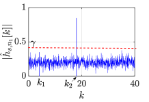
(a)

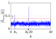
(b)

Figure 3: Extraction of ToA from digital impulse response measured at two points that are spatially close. In (a), the ToA estimate is proportional to $k_{2}$; whereas in (b), the ToA estimate is proportional to $k_{1}$.

It will be argued next that such a ToA feature does not evolve smoothly over space in presence of multipath, and therefore, this may negatively impact estimation performance, as occurs with LocB cartography; see discussion about Fig. 1 in Sec. I. For simplicity, assume that ${{\color[rgb]{0,0,0}a}}_{{\color[rgb]{0,0,0}l}}[k]=\delta[k]$, where $\delta[k]$ is the Kronecker delta. In this case, one can directly estimate $h_{{{\color[rgb]{0,0,0}l}},n}[k]$ as $\hat{h}_{{{\color[rgb]{0,0,0}l}},n}[k]=y_{{{\color[rgb]{0,0,0}l}},n}[k]=h_{{{\color[rgb]{0,0,0}l}},n}[k]+{{\color[rgb]{0,0,0}w}}_{{{\color[rgb]{0,0,0}l}},n}[k]$, which is a noisy version of $h_{{{\color[rgb]{0,0,0}l}},n}[k]$. To see the impact of multipath, consider a simple example where the measurement points $\bm{x}_{n_{1}}$ and $\bm{x}_{n_{2}}$ lie close to each other and the channel impulse responses are given by $\hat{h}_{{{\color[rgb]{0,0,0}l}},n_{1}}[k]={\alpha}_{{{\color[rgb]{0,0,0}l}},n_{1}}^{(1)}\delta[k-k_{{{\color[rgb]{0,0,0}l}},n_{1}}^{(1)}]+{\alpha}_{{{\color[rgb]{0,0,0}l}},n_{1}}^{(2)}\delta[k-k_{{{\color[rgb]{0,0,0}l}},n_{1}}^{(2)}]+{{\color[rgb]{0,0,0}w}}_{{{\color[rgb]{0,0,0}l}},n_{1}}[k]$ and $\hat{h}_{{{\color[rgb]{0,0,0}l}},n_{2}}[k]={\alpha}_{{{\color[rgb]{0,0,0}l}},n_{2}}^{(1)}\delta[k-k_{{{\color[rgb]{0,0,0}l}},n_{2}}^{(1)}]+{\alpha}_{{{\color[rgb]{0,0,0}l}},n_{2}}^{(2)}\delta[k-k_{{{\color[rgb]{0,0,0}l}},n_{2}}^{(2)}]+{{\color[rgb]{0,0,0}w}}_{{{\color[rgb]{0,0,0}l}},n_{2}}[k]$. Due to their spatial proximity, it follows that:

$${\alpha}_{{{\color[rgb]{0,0,0}l}},n_{1}}^{(1)}\approx{\alpha}_{{{\color[rgb]{0,0,0}l}},n_{2}}^{(1)},\quad {\alpha}_{{{\color[rgb]{0,0,0}l}},n_{1}}^{(2)}\approx{\alpha}_{{{\color[rgb]{0,0,0}l}},n_{2}}^{(2)},$$ (14a)

$$k_{{{\color[rgb]{0,0,0}l}},n_{1}}^{(1)}\approx k_{{{\color[rgb]{0,0,0}l}},n_{2}}^{(1)}\approx k_{1},\quad k_{{{\color[rgb]{0,0,0}l}},n_{1}}^{(2)}\approx k_{{{\color[rgb]{0,0,0}l}},n_{2}}^{(2)}\approx k_{2},$$ (14b)

for some $k_{1}$ and $k_{2}$. Assuming for simplicity that the effects of noise are negligible, if $|{\alpha}_{{{\color[rgb]{0,0,0}l}},n_{1}}^{(1)}|<{{\color[rgb]{0,0,0}\gamma}}<|{\alpha}_{{{\color[rgb]{0,0,0}l}},n_{1}}^{(2)}|$ and ${{\color[rgb]{0,0,0}\gamma}}<|{\alpha}_{{{\color[rgb]{0,0,0}l}},n_{2}}^{(1)}|$, then the ToA estimates are:

$$\hat{{\color[rgb]{0,0,0}\tau}}_{n_{1}} :=T\cdot\min\{k:|\hat{h}_{{{\color[rgb]{0,0,0}l}},n_{1}}[k]|\geq{{\color[rgb]{0,0,0}\gamma}}\}=Tk_{{{\color[rgb]{0,0,0}l}},n_{1}}^{(2)}\approx Tk_{2},$$

$$\hat{{\color[rgb]{0,0,0}\tau}}_{n_{2}} :=T\cdot\min\{k:|\hat{h}_{{{\color[rgb]{0,0,0}l}},n_{2}}[k]|\geq{{\color[rgb]{0,0,0}\gamma}}\}=Tk_{{{\color[rgb]{0,0,0}l}},n_{2}}^{(1)}\approx Tk_{1}.$$

This scenario is illustrated in Fig. 3. Despite how close their locations and observed impulse responses are, the ToA estimates at locations $\bm{x}_{n_{1}}$ and $\bm{x}_{n_{2}}$ can be quite different, which establishes that the ToA estimate in (13) is not a smooth function of the spatial location.

Since this non-smoothness negatively affects the performance of the proposed LocF cartography estimator (and since the latter does not need ToA estimates that are proportional to the distance, as occurs in LocB cartography), a promising candidate for feature would be the center of mass (CoM) of the estimated impulse response:

$${\color[rgb]{0,0,0}\text{CoM}}_{{{\color[rgb]{0,0,0}l}},n}:=\frac{\sum_{k=0}^{K-1}|\hat{h}_{{{\color[rgb]{0,0,0}l}},n}[k]|^{2}k}{\sum_{k=0}^{K-1}|\hat{h}_{{{\color[rgb]{0,0,0}l}},n}[k]|^{2}},$$

where $K$ is the number of samples. To see why such a feature evolves smoothly over space, suppose that the effects of noise are negligible and note that this CoM feature applied to the channel impulse responses in the previous example yields:

$${\color[rgb]{0,0,0}\text{CoM}}_{{{\color[rgb]{0,0,0}l}},n_{1}} =\frac{k_{{{\color[rgb]{0,0,0}l}},n_{1}}^{(1)}|\alpha_{{{\color[rgb]{0,0,0}l}},n_{1}}^{(1)}|^{2}+k_{{{\color[rgb]{0,0,0}l}},n_{1}}^{(2)}|\alpha_{{{\color[rgb]{0,0,0}l}},n_{1}}^{(2)}|^{2}}{|\alpha_{{{\color[rgb]{0,0,0}l}},n_{1}}^{(1)}|^{2}+|\alpha_{{{\color[rgb]{0,0,0}l}},n_{1}}^{(2)}|^{2}},$$

$${\color[rgb]{0,0,0}\text{CoM}}_{{{\color[rgb]{0,0,0}l}},n_{2}} =\frac{k_{{{\color[rgb]{0,0,0}l}},n_{2}}^{(1)}|\alpha_{{{\color[rgb]{0,0,0}l}},n_{2}}^{(1)}|^{2}+k_{{{\color[rgb]{0,0,0}l}},n_{2}}^{(2)}|\alpha_{{{\color[rgb]{0,0,0}l}},n_{2}}^{(2)}|^{2}}{|\alpha_{{{\color[rgb]{0,0,0}l}},n_{2}}^{(1)}|^{2}+|\alpha_{{{\color[rgb]{0,0,0}l}},n_{2}}^{(2)}|^{2}}.$$

From (14), it follows that ${\color[rgb]{0,0,0}\text{CoM}}_{{{\color[rgb]{0,0,0}l}},n_{1}}\approx{\color[rgb]{0,0,0}\text{CoM}}_{{{\color[rgb]{0,0,0}l}},n_{2}}$, which indicates that the CoM is indeed a feature that evolves smoothly over space, and therefore preferable for LocF cartography. In this case, the feature vector at the $n$-th sensor location becomes ${\color[rgb]{0,0,0}\bm{\phi}}_{n}=[{\color[rgb]{0,0,0}\text{CoM}}_{1,n},\ldots,{\color[rgb]{0,0,0}\text{CoM}}_{{{\color[rgb]{0,0,0}L}},n}]^{\top}$.

IV-A2 Sensors are not Synchronized with Base Stations

Since synchronization requires more expensive equipment and becomes challenging in multipath scenarios, TDoA estimates are generally preferred for localization. TDoA estimates are typically obtained by extracting the lag corresponding to the maximum cross-correlation of a pair of received pilot signals [38]. Assuming zero-mean, the cross-correlation between two pilot signals received by the sensor at the $n$-th location is defined as:

$$c_{{{\color[rgb]{0,0,0}l}},{{\color[rgb]{0,0,0}l}}^{\prime},n}[{{\color[rgb]{0,0,0}i}}]:=\mathbb{E}\{y_{{{\color[rgb]{0,0,0}l}},n}[k]y_{{{\color[rgb]{0,0,0}l}}^{\prime},n}^{*}[k-{{\color[rgb]{0,0,0}i}}]\}\quad\text{with}\quad{{\color[rgb]{0,0,0}l}}\neq{{\color[rgb]{0,0,0}l}}^{\prime}.$$ (15)

With ${{\color[rgb]{0,0,0}a}}_{{\color[rgb]{0,0,0}l}}[k]={{\color[rgb]{0,0,0}a}}_{{{\color[rgb]{0,0,0}l}}^{\prime}}[k]$ a white process with power $\sigma_{{\color[rgb]{0,0,0}a}}^{2}$ and uncorrelated with ${{\color[rgb]{0,0,0}w}}_{{{\color[rgb]{0,0,0}l}},n}[k]$ and ${{\color[rgb]{0,0,0}w}}_{{{\color[rgb]{0,0,0}l}}^{\prime},n}[k]$, also uncorrelated with each other, it can be easily seen that:

$$c_{{{\color[rgb]{0,0,0}l}},{{\color[rgb]{0,0,0}l}}^{\prime},n}[{{\color[rgb]{0,0,0}i}}]=\sigma_{{{\color[rgb]{0,0,0}a}}}^{2}\left(h_{{{\color[rgb]{0,0,0}l}},n}[{{\color[rgb]{0,0,0}i}}]\ast h_{{{\color[rgb]{0,0,0}l}}^{\prime},n}^{*}[-{{\color[rgb]{0,0,0}i}}]\right).$$

A common estimate of the TDoA ${{{\color[rgb]{0,0,0}\Delta}}}_{{{\color[rgb]{0,0,0}l}},{{\color[rgb]{0,0,0}l}}^{\prime},n}$ is (see e.g. [38]):

$$\hat{{{\color[rgb]{0,0,0}\Delta}}}_{{{\color[rgb]{0,0,0}l}},{{\color[rgb]{0,0,0}l}}^{\prime},n}=T\cdot\arg\max_{{{\color[rgb]{0,0,0}i}}}\{\left|\hat{c}_{{{\color[rgb]{0,0,0}l}},{{\color[rgb]{0,0,0}l}}^{\prime},n}[{{\color[rgb]{0,0,0}i}}]\right|\},$$ (16)

where $\hat{c}_{{{\color[rgb]{0,0,0}l}},{{\color[rgb]{0,0,0}l}}^{\prime},n}[{{\color[rgb]{0,0,0}i}}]$ is an estimate of $c_{{{\color[rgb]{0,0,0}l}},{{\color[rgb]{0,0,0}l}}^{\prime},n}[{{\color[rgb]{0,0,0}i}}]$. To see the intuition behind this estimator, note that $\hat{h}_{{{\color[rgb]{0,0,0}l}},n}[k]={\alpha}_{{{\color[rgb]{0,0,0}l}},n}^{(1)}\delta[k-k_{{{\color[rgb]{0,0,0}l}},n}^{(1)}]$ and $\hat{h}_{{{\color[rgb]{0,0,0}l}}^{\prime},n}[k]={\alpha}_{{{\color[rgb]{0,0,0}l}}^{\prime},n}^{(1)}\delta[k-k_{{{\color[rgb]{0,0,0}l}}^{\prime},n}^{(1)}]$ in a free-space channel with large bandwidth $B$. This implies that:

$$c_{{{\color[rgb]{0,0,0}l}},{{\color[rgb]{0,0,0}l}}^{\prime},n}[{{\color[rgb]{0,0,0}i}}] =\sigma_{{{\color[rgb]{0,0,0}a}}}^{2}{\alpha}_{{{\color[rgb]{0,0,0}l}},n}^{(1)}\left({\alpha}_{{{\color[rgb]{0,0,0}l}}^{\prime},n}^{(1)}\right)^{*}\delta\left[{{\color[rgb]{0,0,0}i}}-\left(k_{{{\color[rgb]{0,0,0}l}},n}^{(1)}-k_{{{\color[rgb]{0,0,0}l}}^{\prime},n}^{(1)}\right)\right]$$

$$=\sigma_{{{\color[rgb]{0,0,0}a}}}^{2}{\alpha}_{{{\color[rgb]{0,0,0}l}},n}^{(1)}\left({\alpha}_{{{\color[rgb]{0,0,0}l}}^{\prime},n}^{(1)}\right)^{*}\delta\left[{{\color[rgb]{0,0,0}i}}-{{\color[rgb]{0,0,0}\Delta}}_{{{\color[rgb]{0,0,0}l}},{{\color[rgb]{0,0,0}l}}^{\prime},n}/T\right],$$

and therefore the lag of the maximum magnitude of $c_{{{\color[rgb]{0,0,0}l}},{{\color[rgb]{0,0,0}l}}^{\prime},n}[{{\color[rgb]{0,0,0}i}}]$ provides the TDoA in this simple scenario.

Similar arguments to those used in Sec. IV-A1 to conclude that the ToA estimates are not spatially smooth can also be invoked to reach the same conclusion for TDoA. Likewise, following the same rationale as in Sec. IV-A1, this section proposes alleviating the aforementioned issue by adopting features of the form:

$${\color[rgb]{0,0,0}\text{CoM}}_{{{\color[rgb]{0,0,0}l}},{{\color[rgb]{0,0,0}l}}^{\prime},n}:=\frac{\sum_{{{\color[rgb]{0,0,0}i}}=-K+1}^{K-1}|c_{{{\color[rgb]{0,0,0}l}},{{\color[rgb]{0,0,0}l}}^{\prime},n}[{{\color[rgb]{0,0,0}i}}]|^{2}~{}{{{\color[rgb]{0,0,0}i}}}}{\sum_{{{\color[rgb]{0,0,0}i}}=-K+1}^{K-1}|c_{{{\color[rgb]{0,0,0}l}},{{\color[rgb]{0,0,0}l}}^{\prime},n}[{{\color[rgb]{0,0,0}i}}]|^{2}},$$ (17)

where ${\color[rgb]{0,0,0}\text{CoM}}_{{{\color[rgb]{0,0,0}l}},{{\color[rgb]{0,0,0}l}}^{\prime},n}$ is the CoM of the cross-correlation between the ${{{\color[rgb]{0,0,0}l}}}$-th and ${{{\color[rgb]{0,0,0}l}}^{\prime}}$-th pilot signals. The proposed feature has three advantages: i) it is smooth, as portrayed later in Sec. V-A, ii) it does not require synchronization between the localization base stations and the sensors, and iii) it does not require the knowledge of the impulse responses. With this choice, the feature vector at the $n$-th measurement location becomes:

$$\begin{split}{\color[rgb]{0,0,0}\bm{\phi}}_{n}=&[{\color[rgb]{0,0,0}\text{CoM}}_{1,2,n},{\color[rgb]{0,0,0}\text{CoM}}_{1,3,n},\ldots,{\color[rgb]{0,0,0}\text{CoM}}_{1,{{\color[rgb]{0,0,0}L}},n},\\ &{\color[rgb]{0,0,0}\text{CoM}}_{2,3,n},\ldots,{\color[rgb]{0,0,0}\text{CoM}}_{{{\color[rgb]{0,0,0}L}}-1,{{\color[rgb]{0,0,0}L}},n}]^{\top}.\end{split}$$ (18)

IV-B Cartography from a Reduced Set of Features

As argued earlier in Sec. III-A, learning becomes difficult when the number of input features ${{\color[rgb]{0,0,0}M}}$ is high. This section develops a scheme to reduce this number of features to improve estimation performance in LocF cartography.

As stated in the previous section, in LocB cartography, the feature vectors correspond to the coordinates of the estimated location. Application of the localization algorithm represented by the function ${\hat{\bm{l}}}$ in (LABEL:eq:locasedFeat) naturally reduces dimensionality from the original ${{\color[rgb]{0,0,0}M}}$ features to just 2 or 3. On the other hand, in the case of LocF cartography, a larger number $N$ of measurements to learn ${{\color[rgb]{0,0,0}\hat{d}}}$ in (LABEL:eq:locFree) may be necessary to attain a target accuracy if ${{\color[rgb]{0,0,0}M}}$ is large. This observation calls for a dimensionality reduction step that condenses the information of the feature vectors $\{{\color[rgb]{0,0,0}\bm{\phi}}_{n}\}_{n=1}^{N}\subset\mathbb{R}^{{\color[rgb]{0,0,0}M}}$ into vectors $\{{{\color[rgb]{0,0,0}{\bar{\bm{\phi}}}}}_{n}\}_{n=1}^{N}\subset\mathbb{R}^{{{{\color[rgb]{0,0,0}r}}}}$ of a reduced size ${{{\color[rgb]{0,0,0}r}}}$.

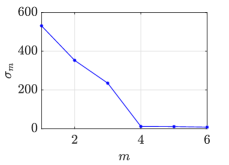
Figure 4: Singular values $\sigma_{1}\geq\sigma_{2}\geq\ldots\geq\sigma_{{{\color[rgb]{0,0,0}M}}}\geq 0$ of ${\color[rgb]{0,0,0}\bm{\Phi}}$ in non-increasing order for a multipath environment with ${{\color[rgb]{0,0,0}L}}=4$ transmitters.

Intuitively, ${{{\color[rgb]{0,0,0}r}}}$ should be the minimum number that preserves most information while eliminating most of the noise in $\{{\color[rgb]{0,0,0}\bm{\phi}}_{n}\}_{n=1}^{N}$. Even if some information is lost, the reduction in the error entailed by the fact that the function to be estimated has fewer input arguments may pay off in practice.

In the cases where the feature vectors $\{{\color[rgb]{0,0,0}\bm{\phi}}_{n}\}_{n=1}^{N}$ lie close to a low-dimensional subspace, the coordinates of these vectors with respect to a basis for such a subspace may constitute a suitable reduced set of features. To see this, it is instructive to start by considering the scenario of TDoA features. Suppose, for simplicity, that the effects of noise are negligible, so that the TDoA estimates $\hat{{{\color[rgb]{0,0,0}\Delta}}}_{{{\color[rgb]{0,0,0}l}},{{\color[rgb]{0,0,0}l}}^{\prime},n}$ approximately equal the true TDoAs ${{{\color[rgb]{0,0,0}\Delta}}}_{{{\color[rgb]{0,0,0}l}},{{\color[rgb]{0,0,0}l}}^{\prime},n}$. Then, the rows of ${\color[rgb]{0,0,0}\bm{\Phi}}:=[{\color[rgb]{0,0,0}\bm{\phi}}_{1},\ldots,{\color[rgb]{0,0,0}\bm{\phi}}_{N}]$ are of the form $\bm{{{\color[rgb]{0,0,0}\Delta}}}_{{{{\color[rgb]{0,0,0}l}}},{{{\color[rgb]{0,0,0}l}}^{\prime}}}:=[{{\color[rgb]{0,0,0}\Delta}}_{{{\color[rgb]{0,0,0}l}},{{\color[rgb]{0,0,0}l}}^{\prime},1},{{\color[rgb]{0,0,0}\Delta}}_{{{\color[rgb]{0,0,0}l}},{{\color[rgb]{0,0,0}l}}^{\prime},2},\ldots,{{\color[rgb]{0,0,0}\Delta}}_{{{\color[rgb]{0,0,0}l}},{{\color[rgb]{0,0,0}l}}^{\prime},N}]^{\top}$. If $\bm{{{\color[rgb]{0,0,0}\tau}}}_{{{\color[rgb]{0,0,0}l}}}:=[{{\color[rgb]{0,0,0}\tau}}_{{{\color[rgb]{0,0,0}l}},1},\ldots,{{\color[rgb]{0,0,0}\tau}}_{{{\color[rgb]{0,0,0}l}},N}]^{\top}$ collects the ToA from the ${{\color[rgb]{0,0,0}l}}$-th base station to all sensor locations, then it clearly holds that $\bm{{{\color[rgb]{0,0,0}\Delta}}}_{{{\color[rgb]{0,0,0}l}},{{\color[rgb]{0,0,0}l}}^{\prime}}={{\color[rgb]{0,0,0}\bm{\tau}}}_{{{\color[rgb]{0,0,0}l}}}-{{\color[rgb]{0,0,0}\bm{\tau}}}_{{{\color[rgb]{0,0,0}l}}^{\prime}}$. Consequently, $\bm{{{\color[rgb]{0,0,0}\Delta}}}_{1,{{\color[rgb]{0,0,0}l}}}-\bm{{{\color[rgb]{0,0,0}\Delta}}}_{1,{{\color[rgb]{0,0,0}l}}^{\prime}}={{\color[rgb]{0,0,0}\bm{\tau}}}_{1}-{{\color[rgb]{0,0,0}\bm{\tau}}}_{{{\color[rgb]{0,0,0}l}}}-({{\color[rgb]{0,0,0}\bm{\tau}}}_{1}-{{\color[rgb]{0,0,0}\bm{\tau}}}_{{{\color[rgb]{0,0,0}l}}^{\prime}})={{\color[rgb]{0,0,0}\bm{\tau}}}_{{{\color[rgb]{0,0,0}l}}^{\prime}}-{{\color[rgb]{0,0,0}\bm{\tau}}}_{{{\color[rgb]{0,0,0}l}}}=\bm{{{\color[rgb]{0,0,0}\Delta}}}_{{{\color[rgb]{0,0,0}l}}^{\prime},{{\color[rgb]{0,0,0}l}}}$, which implies that all rows of ${\color[rgb]{0,0,0}\bm{\Phi}}$ are linear combinations of the ${{\color[rgb]{0,0,0}L}}-1$ rows $\{\bm{{{\color[rgb]{0,0,0}\Delta}}}_{1,{{\color[rgb]{0,0,0}l}}}\}_{{{\color[rgb]{0,0,0}l}}=2}^{{\color[rgb]{0,0,0}L}}$. Thus, the rank of ${\color[rgb]{0,0,0}\bm{\Phi}}$ is at most ${{\color[rgb]{0,0,0}L}}-1$ or, equivalently, the vectors $\{{\color[rgb]{0,0,0}\bm{\phi}}_{n}\}_{n=1}^{N}$ lie in a subspace of dimension ${{\color[rgb]{0,0,0}L}}-1$. When effects of noise are noticeable, one would expect that the vectors $\{{\color[rgb]{0,0,0}\bm{\phi}}_{n}\}_{n=1}^{N}$ lie close to a subspace of dimension ${{\color[rgb]{0,0,0}L}}-1$.

Similarly, one can expect that when the entries of the vectors $\{{\color[rgb]{0,0,0}\bm{\phi}}_{n}\}_{n=1}^{N}$ are given by (17), these vectors also lie close to a low-dimensional subspace since CoM features are proportional to the TDoAs in absence of multipath; see Sec. IV-A. This phenomenon can be illustrated through simulation (see Sec. V for more details). Fig. 4 depicts the singular values $\sigma_{1}\geq\sigma_{2}\geq\ldots\geq\sigma_{{{\color[rgb]{0,0,0}M}}}\geq 0$ of ${\color[rgb]{0,0,0}\bm{\Phi}}$ in non-increasing order for a multipath environment described in Sec. V with ${{\color[rgb]{0,0,0}L}}=4$. As expected, roughly ${{{\color[rgb]{0,0,0}r}}}={{\color[rgb]{0,0,0}L}}-1=3$ directions capture almost all the energy of the rows of ${\color[rgb]{0,0,0}\bm{\Phi}}$.

When a set of random vectors lie close to a subspace, an appealing approach for dimensionality reduction is principal component analysis (PCA) [32, Ch. 12], which obtains the reduced feature vectors by projecting the input data vectors onto the subspace that preserves most of the energy. Since in this paper no probabilistic assumptions have been introduced on $\{{\color[rgb]{0,0,0}\bm{\phi}}_{n}\}_{n=1}^{N}$, the typical formulation of PCA is not directly applicable. However, as detailed next, it is not difficult to extend this idea to the fully deterministic scenario, which furthermore provides intuition.

Assume w.l.o.g. a centered set of feature vectors, i.e., $({1/N})\sum_{n=1}^{N}{\color[rgb]{0,0,0}\bm{\phi}}_{n}=\bm{0}$. If not centered, just subtract the mean by replacing ${\color[rgb]{0,0,0}\bm{\Phi}}$ with ${\color[rgb]{0,0,0}\bm{\Phi}}-(1/N){\color[rgb]{0,0,0}\bm{\Phi}}\bm{1}\bm{1}^{\top}$. The subspace that captures most of the energy of the observations can be determined using the singular value decomposition (SVD) of ${\color[rgb]{0,0,0}\bm{\Phi}}$, which for ${{\color[rgb]{0,0,0}M}}<N$ is given by:

$${\color[rgb]{0,0,0}\bm{\Phi}}=\begin{bmatrix}\bm{U}_{1}&\bm{U}_{2}\end{bmatrix}\left[\begin{array}[]{@{}c|c@{}}\begin{matrix}\bm{\Sigma}_{1}&\bm{0}\\ \ \bm{0}&\bm{\Sigma}_{2}\end{matrix}\end{array}\begin{matrix}\ \bm{0}\\ \ \bm{0}\end{matrix}\right]\begin{bmatrix}\bm{V}_{1}^{\top}\\ \ \bm{V}_{2}^{\top}\end{bmatrix},$$ (20)

where $\bm{\Sigma}_{1}:=\mathop{\rm diag}\left\{\sigma_{1},\ldots,\sigma_{{{{\color[rgb]{0,0,0}r}}}}\right\}$ contains the ${{{\color[rgb]{0,0,0}r}}}$ largest singular values of ${\color[rgb]{0,0,0}\bm{\Phi}}$, $\bm{\Sigma}_{2}:=\mathop{\rm diag}\left\{\sigma_{{{{\color[rgb]{0,0,0}r}}}+1},\ldots,\sigma_{{{\color[rgb]{0,0,0}M}}}\right\}$ contains the ${{\color[rgb]{0,0,0}M}}-{{{\color[rgb]{0,0,0}r}}}$ smallest, and the columns of $\bm{U}:=\begin{bmatrix}\bm{U}_{1}&\bm{U}_{2}\end{bmatrix}$ (respectively $\bm{V}:=[\bm{V}_{1},\bm{V}_{2}]$) are the left (right) singular vectors of ${\color[rgb]{0,0,0}\bm{\Phi}}$. Clearly, if the data vectors $\{{\color[rgb]{0,0,0}\bm{\phi}}_{n}\}_{n=1}^{N}$ are multiplied by the orthogonal matrix $\bm{U}^{\top}$, the resulting vectors $\{{{\color[rgb]{0,0,0}\bm{\phi}^{\prime}}}_{n}\}_{n=1}^{N}$, with ${{\color[rgb]{0,0,0}\bm{\phi}^{\prime}}}_{n}:=\bm{U}^{\top}{\color[rgb]{0,0,0}\bm{\phi}}_{n}$, contain the same information. Thus, one can replace ${\color[rgb]{0,0,0}\bm{\Phi}}$ with ${{\color[rgb]{0,0,0}\bm{\Phi}^{\prime}}}:=\bm{U}^{\top}{\color[rgb]{0,0,0}\bm{\Phi}}$.

By applying this transformation, which can be thought of as a generalized rotation, most of the energy of ${{\color[rgb]{0,0,0}\bm{\Phi}^{\prime}}}$ is concentrated in its first ${{{\color[rgb]{0,0,0}r}}}$ rows. To see this, note that the energy of the first ${{{\color[rgb]{0,0,0}r}}}$ rows of ${{\color[rgb]{0,0,0}\bm{\Phi}^{\prime}}}$ is given by:

$$||\bm{U}_{1}^{\top}{\color[rgb]{0,0,0}\bm{\Phi}}||_{F}^{2} =||\bm{\Sigma}_{1}\bm{V}_{1}^{\top}||_{F}^{2}=\mathrm{Tr}\left(\bm{\Sigma}_{1}\bm{V}_{1}^{\top}\bm{V}_{1}\bm{\Sigma}_{1}^{\top}\right)$$

$$=\mathrm{Tr}\left(\bm{\Sigma}_{1}\bm{\Sigma}_{1}^{\top}\right)=||\bm{\Sigma}_{1}||_{F}^{2}=\sum_{{{\color[rgb]{0,0,0}m}}=1}^{{{\color[rgb]{0,0,0}r}}}\sigma_{{\color[rgb]{0,0,0}m}}^{2},$$

whereas the energy of the last ${{\color[rgb]{0,0,0}M}}-{{{\color[rgb]{0,0,0}r}}}$ rows of ${{\color[rgb]{0,0,0}\bm{\Phi}^{\prime}}}$ is given by:

$$||\bm{U}_{2}^{\top}{\color[rgb]{0,0,0}\bm{\Phi}}||_{F}^{2}=||\bm{\Sigma}_{2}||_{F}^{2}=\sum_{{{\color[rgb]{0,0,0}m}}={{{\color[rgb]{0,0,0}r}}}+1}^{{\color[rgb]{0,0,0}M}}\sigma_{{\color[rgb]{0,0,0}m}}^{2}.$$

When ${{{\color[rgb]{0,0,0}r}}}={{\color[rgb]{0,0,0}L}}-1$, since the rows of ${\color[rgb]{0,0,0}\bm{\Phi}}$ lie approximately in a subspace of dimension ${{{\color[rgb]{0,0,0}r}}}$, it follows that $\sigma_{{\color[rgb]{0,0,0}m}}\approx 0$ for ${{\color[rgb]{0,0,0}m}}>{{{\color[rgb]{0,0,0}r}}}$. Therefore $\sum_{{{\color[rgb]{0,0,0}m}}=1}^{{{\color[rgb]{0,0,0}r}}}\sigma_{{\color[rgb]{0,0,0}m}}^{2}\gg\sum_{{{\color[rgb]{0,0,0}m}}={{{\color[rgb]{0,0,0}r}}}+1}^{{\color[rgb]{0,0,0}M}}\sigma_{{\color[rgb]{0,0,0}m}}^{2}$ and, hence, $||\bm{U}_{1}^{\top}{\color[rgb]{0,0,0}\bm{\Phi}}||_{F}^{2}\gg||\bm{U}_{2}^{\top}{\color[rgb]{0,0,0}\bm{\Phi}}||_{F}^{2}$. Equivalently, most of the energy of the vectors $\{{{\color[rgb]{0,0,0}\bm{\phi}^{\prime}}}_{n}\}_{n=1}^{N}$ is concentrated in their first ${{{\color[rgb]{0,0,0}r}}}$ entries. This observation suggests using the first ${{{\color[rgb]{0,0,0}r}}}$ entries of the vectors $\{{{\color[rgb]{0,0,0}\bm{\phi}^{\prime}}}_{n}\}_{n=1}^{N}$ as features, while discarding the rest. That is, the reduced dimensionality feature vectors will be given by $\{{{\color[rgb]{0,0,0}{\bar{\bm{\phi}}}}}_{n}\}_{n=1}^{N}$, where ${{\color[rgb]{0,0,0}{\bar{\bm{\phi}}}}}_{n}:=\bm{U}_{1}^{\top}{\color[rgb]{0,0,0}\bm{\phi}}_{n}$. Note that ${{\color[rgb]{0,0,0}{\bar{\bm{\phi}}}}}_{n}$ is just the vector of coordinates of ${\color[rgb]{0,0,0}\bm{\phi}}_{n}$ with respect to the basis composed of the columns of $\bm{U}_{1}$.

The number ${{{\color[rgb]{0,0,0}r}}}$ of entries of the new feature vectors $\{{{\color[rgb]{0,0,0}{\bar{\bm{\phi}}}}}_{n}\}_{n=1}^{N}$ may be potentially much smaller than ${{\color[rgb]{0,0,0}M}}$ and can therefore boost estimation performance meaningfully. For instance, when $\{{\color[rgb]{0,0,0}\bm{\phi}}_{n}\}_{n=1}^{N}$ are given by (18), this reduction is from ${{\color[rgb]{0,0,0}M}}={{\color[rgb]{0,0,0}L}}({{\color[rgb]{0,0,0}L}}-1)/2$ features to ${{{\color[rgb]{0,0,0}r}}}={{\color[rgb]{0,0,0}L}}-1$ features.

In scenarios of very strong multipath, the rows of ${\color[rgb]{0,0,0}\bm{\Phi}}$ may not lie close to any subspace of dimension ${{\color[rgb]{0,0,0}L}}-1$. In those cases, it may be worth choosing a value of ${{{\color[rgb]{0,0,0}r}}}$ greater than ${{\color[rgb]{0,0,0}L}}-1$. A possibility is to specify a fraction ${{\color[rgb]{0,0,0}\eta}}\in[0,1]$ of the energy of ${\color[rgb]{0,0,0}\bm{\Phi}}$ that must be kept in ${{\color[rgb]{0,0,0}{\bar{\bm{\Phi}}}}}:=\bm{U}_{1}^{\top}{\color[rgb]{0,0,0}\bm{\Phi}}$, and choose ${{{\color[rgb]{0,0,0}r}}}$ to be the smallest integer that guarantees this condition, that is:

$${{{\color[rgb]{0,0,0}r}}}=\min\left\{{{{\color[rgb]{0,0,0}r}}}^{\prime}:\frac{\sum_{{{\color[rgb]{0,0,0}\bar{m}}}=1}^{{{{\color[rgb]{0,0,0}r}}}^{\prime}}\sigma_{{{\color[rgb]{0,0,0}\bar{m}}}}^{2}}{\sum_{{{\color[rgb]{0,0,0}m}}=1}^{{\color[rgb]{0,0,0}M}}\sigma_{{{\color[rgb]{0,0,0}m}}}^{2}}\geq{{\color[rgb]{0,0,0}\eta}}\right\}.$$ (21)

To summarize, the problem of LocF cartography with the technique for reducing the set of features introduced in this section is as follows. Given the original set of measurements $\{{\color[rgb]{0,0,0}\bm{\phi}}_{n}\}_{n=1}^{N}\subset\mathbb{R}^{{\color[rgb]{0,0,0}M}}$, one must form the matrix ${\color[rgb]{0,0,0}\bm{\Phi}}$, compute $\bm{U}_{1}$ from the SVD in (20), and obtain the reduced features $\{{{\color[rgb]{0,0,0}{\bar{\bm{\phi}}}}}_{n}\}_{n=1}^{N}\subset\mathbb{R}^{{{{\color[rgb]{0,0,0}r}}}}$ where ${{\color[rgb]{0,0,0}{\bar{\bm{\phi}}}}}_{n}=\bm{U}_{1}^{\top}{\color[rgb]{0,0,0}\bm{\phi}}_{n}$. Then, the function ${{\color[rgb]{0,0,0}\hat{d}}}$ is obtained form the pairs $\{({{\color[rgb]{0,0,0}{\bar{\bm{\phi}}}}}_{n},\tilde{p}_{n})\}_{n=1}^{N}$ using the approach in Sec. III-B. To evaluate the resulting map at a query location where the received pilot signals are given by ${\color[rgb]{0,0,0}\bm{Y}}$, one must simply obtain ${{\color[rgb]{0,0,0}\hat{d}}}(\bm{U}_{1}^{\top}{\color[rgb]{0,0,0}\bm{\phi}}(\bm{Y}))$.

IV-C Dealing with Missing Features

Due to propagation effects, the signal-to-noise ratio of some of the received pilot signals may be too low for feature extraction. In this case, the features associated with those pilot signals may be unreliable or simply unavailable. This section develops techniques to cope with such missing features.

Let $\Omega\subset\{1,\ldots,{{\color[rgb]{0,0,0}M}}\}\times\{1,\ldots,N\}$ be such that $({{\color[rgb]{0,0,0}m}},n)\in\Omega$ iff the ${{\color[rgb]{0,0,0}m}}$-th feature is available at the $n$-th measurement location and define the “incomplete” feature matrix ${{\color[rgb]{0,0,0}\breve{\bm{\Phi}}}}~{}\in\left(\mathbb{R}\cup\{{\color[rgb]{0,0,0}\text{FiM}}\}\right)^{{{\color[rgb]{0,0,0}M}}\times N}$ as:

$$({{\color[rgb]{0,0,0}\breve{\bm{\Phi}}}})_{{{\color[rgb]{0,0,0}m}},n}=\begin{cases}({\color[rgb]{0,0,0}\bm{\phi}}_{n})_{{{\color[rgb]{0,0,0}m}}}+\varsigma_{{{\color[rgb]{0,0,0}m}},n}&\text{if}~{}({{\color[rgb]{0,0,0}m}},n)\in\Omega\\ {\color[rgb]{0,0,0}\text{FiM}}&\text{otherwise},\end{cases}$$ (22)

where $\varsigma_{{{\color[rgb]{0,0,0}m}},n}$ explicitly models error in the feature extraction and the symbol FiM represents that the corresponding feature is missing. Since the matrix ${{\color[rgb]{0,0,0}\breve{\bm{\Phi}}}}$ contains missing features, the LocF cartography scheme presented so far is not directly applicable. The missing features must be filled first. Hence, the goal is, given ${{\color[rgb]{0,0,0}\breve{\bm{\Phi}}}}$, find ${\color[rgb]{0,0,0}\bm{\Phi}}\in\mathbb{R}^{{{\color[rgb]{0,0,0}M}}\times N}$ that agrees with ${{\color[rgb]{0,0,0}\breve{\bm{\Phi}}}}$ on $\Omega$. A popular approach to address such a matrix completion task is via rank minimization [39]:

$$\begin{split}&\underset{{\color[rgb]{0,0,0}\bm{\Phi}}}{\text{minimize}}\quad\text{rank}\left({\color[rgb]{0,0,0}\bm{\Phi}}\right)\\ &\text{subject to}\quad\mathcal{P}_{\Omega}({\color[rgb]{0,0,0}\bm{\Phi}})=\mathcal{P}_{\Omega}({{\color[rgb]{0,0,0}\breve{\bm{\Phi}}}}),\end{split}$$ (23)

where

$$\begin{aligned} &\mathcal{P}_{\Omega}:&\left(\mathbb{R}\cup\{{\color[rgb]{0,0,0}\text{FiM}}\}\right)^{{{\color[rgb]{0,0,0}M}}\times N}&\longrightarrow\mathbb{R}^{{{\color[rgb]{0,0,0}M}}\times N}\\ &&{{\color[rgb]{0,0,0}\breve{\bm{\Phi}}}}&\longmapsto\mathcal{P}_{\Omega}({{\color[rgb]{0,0,0}\breve{\bm{\Phi}}}}),\end{aligned}$$

with

$$\left(\mathcal{P}_{\Omega}({{\color[rgb]{0,0,0}\breve{\bm{\Phi}}}})\right)_{{{\color[rgb]{0,0,0}m}},n}=\begin{cases}({{\color[rgb]{0,0,0}\breve{\bm{\Phi}}}})_{{{\color[rgb]{0,0,0}m}},n}&\text{if}~{}({{\color[rgb]{0,0,0}m}},n)\in\Omega\\ 0&\text{if}~{}({{\color[rgb]{0,0,0}m}},n)\notin\Omega.\end{cases}$$

Although this problem is non-convex, efficient solvers exist based on convex relaxation [40, 41]. A legitimate question would be what is the minimum number of available features required to recover a reasonable reconstruction of ${\color[rgb]{0,0,0}\bm{\Phi}}$. As a guideline, a result in [42] establishes that, under certain conditions, the minimum number of available features to recover ${\color[rgb]{0,0,0}\bm{\Phi}}\in\mathbb{R}^{{{\color[rgb]{0,0,0}M}}\times N}$ is $\mathcal{O}\left(\tilde{N}\mathop{\rm rank}({\color[rgb]{0,0,0}\bm{\Phi}})\log(\tilde{N})\right)$ where $\tilde{N}=\max({{\color[rgb]{0,0,0}M}},N)$.

Although the aforementioned rank minimization approach could, in principle, be used, it suffers from two limitations. First, it does not exploit the prior information that ${\color[rgb]{0,0,0}\bm{\Phi}}$ can be well approximated by a matrix of rank ${{\color[rgb]{0,0,0}r}}$, where ${{\color[rgb]{0,0,0}r}}$ is typically ${{\color[rgb]{0,0,0}L}}-1$; see Fig. 4. Second, the constraint in (23) would render the reconstructed matrix sensitive to the noise $\{\varsigma_{{{\color[rgb]{0,0,0}m}},n}\}_{{{\color[rgb]{0,0,0}m}},n}$ present in ${{\color[rgb]{0,0,0}\breve{\bm{\Phi}}}}$. Thus, an appealing alternative to (23) would be:

$$\begin{split}{\color[rgb]{0,0,0}\mathring{\bm{\Phi}}}:=&\underset{{\color[rgb]{0,0,0}\bm{\Phi}}}{\text{argmin}}\quad\frac{1}{2}||\mathcal{P}_{\Omega}({\color[rgb]{0,0,0}\bm{\Phi}})-\mathcal{P}_{\Omega}({{\color[rgb]{0,0,0}\breve{\bm{\Phi}}}})||_{F}^{2}\\ &\text{subject to}\quad{\color[rgb]{0,0,0}\bm{\Phi}}\in\mathcal{M}_{{\color[rgb]{0,0,0}r}},\end{split}$$ (24)

where $\mathcal{M}_{{\color[rgb]{0,0,0}r}}:=\{{\color[rgb]{0,0,0}\bm{\Phi}}\in\mathbb{R}^{{{\color[rgb]{0,0,0}M}}\times N}:\text{rank}({\color[rgb]{0,0,0}\bm{\Phi}})={{\color[rgb]{0,0,0}r}}\}$ is the smooth manifold of ${{\color[rgb]{0,0,0}r}}$-rank ${{\color[rgb]{0,0,0}M}}\times N$ matrices.

There exist algorithms to find local minima of the non-convex problem (24). One example based on manifold optimization [43] is the linear retraction-based geometric conjugate gradient (LRGeomCG) method from [44]. A less computationally expensive alternative is the singular value projection (SVP) method in [45], which is based on the traditional projected subgradient descent method.

After solving (24), all the columns of ${\color[rgb]{0,0,0}\mathring{\bm{\Phi}}}:=[{\color[rgb]{0,0,0}\mathring{\bm{\phi}}}_{1},\ldots,{\color[rgb]{0,0,0}\mathring{\bm{\phi}}}_{N}]$ clearly lie in a subspace of dimension ${{\color[rgb]{0,0,0}r}}$. From the arguments in Sec. IV-B, learning the map can be improved by suppressing this redundancy. To this end, one could use the technique in Sec. IV-B, which would obtain the reduced-dimensionality feature vectors as follows:

$${\color[rgb]{0,0,0}{\bar{\bm{\Phi}}}}:=[{{\color[rgb]{0,0,0}{\bar{\bm{\phi}}}}}_{1},\ldots,{{\color[rgb]{0,0,0}{\bar{\bm{\phi}}}}}_{N}]=\mathring{\bm{U}}_{1}^{\top}{\color[rgb]{0,0,0}\mathring{\bm{\Phi}}}.$$ (25)

Here, the columns of $\mathring{\bm{U}}_{1}$ are the left singular vectors corresponding to the ${{\color[rgb]{0,0,0}r}}$ largest singular values of ${\color[rgb]{0,0,0}\mathring{\bm{\Phi}}}$. Nevertheless, since ${\color[rgb]{0,0,0}\mathring{\bm{\Phi}}}$ has rank ${{\color[rgb]{0,0,0}r}}$, it is not necessary to obtain $\mathring{\bm{U}}_{1}$ by means of an SVD. Namely, the columns of $\mathring{\bm{U}}_{1}$ can be directly obtained by orthonormalizing the first ${{\color[rgb]{0,0,0}r}}$ linearly independent columns of ${\color[rgb]{0,0,0}\mathring{\bm{\Phi}}}$, e.g. through Gram-Schmidt.

To sum up, to estimate a map using the proposed LocF cartography in presence of missing features is as follows. First, matrix ${{\color[rgb]{0,0,0}\breve{\bm{\Phi}}}}$ is formed with the available features. Then, the completed matrix ${\color[rgb]{0,0,0}\mathring{\bm{\Phi}}}$ is obtained using LRGeomCG or SVP. Next, $\mathring{\bm{U}}_{1}$ is obtained through Gram-Schmidt over this completed matrix. Finally, one learns ${{\color[rgb]{0,0,0}\hat{d}}}$ from $\{({{\color[rgb]{0,0,0}{\bar{\bm{\phi}}}}}_{n},\tilde{p}_{n})\}_{n=1}^{N}$, where ${{\color[rgb]{0,0,0}{\bar{\bm{\phi}}}}}_{n}$ is the $n$-th column of ${\color[rgb]{0,0,0}{\bar{\bm{\Phi}}}}$ in (25), using the approach in Sec. III-B.

To evaluate the estimated map at a test location, one would require in principle the feature vector ${\color[rgb]{0,0,0}\bm{\phi}}\in\mathbb{R}^{{\color[rgb]{0,0,0}M}}$ at that location or, alternatively, its reduced-dimensionality version ${{\color[rgb]{0,0,0}{\bar{\bm{\phi}}}}}\in\mathbb{R}^{{\color[rgb]{0,0,0}r}}$. However, due to the phenomena described earlier, only some of the features of ${\color[rgb]{0,0,0}\bm{\phi}}$ may be available, which can be collected in the vector ${{\color[rgb]{0,0,0}\breve{\bm{\phi}}}}\in\left(\mathbb{R}\cup\{{\color[rgb]{0,0,0}\text{FiM}}\}\right)^{{\color[rgb]{0,0,0}M}}$. The problem now is to find the reduced-dimensionality feature vector ${{\color[rgb]{0,0,0}{\bar{\bm{\phi}}}}}$ given ${{\color[rgb]{0,0,0}\breve{\bm{\phi}}}}$.

Since the columns of ${\color[rgb]{0,0,0}\mathring{\bm{\Phi}}}$ lie in an ${{{\color[rgb]{0,0,0}r}}}$-dimensional subspace for which the columns of $\mathring{\bm{U}}_{1}$ form an orthonormal basis, it is reasonable to say that the feature vector at the testing point ${\color[rgb]{0,0,0}\bm{\phi}}\in\mathbb{R}^{{{\color[rgb]{0,0,0}M}}}$ also lies in that subspace, meaning that this vector can be written as ${\color[rgb]{0,0,0}\bm{\phi}}=\mathring{\bm{U}}_{1}{{\color[rgb]{0,0,0}{\bar{\bm{\phi}}}}}$ for some ${{\color[rgb]{0,0,0}{\bar{\bm{\phi}}}}}$. The procedure to recover ${{\color[rgb]{0,0,0}{\bar{\bm{\phi}}}}}$ depends on whether ${{\color[rgb]{0,0,0}\breve{\bm{\phi}}}}$ contains enough observed features. Let $\Omega^{\prime}\subset\{1,\ldots,{{\color[rgb]{0,0,0}M}}\}$ be such that the ${{\color[rgb]{0,0,0}m}}\in\Omega^{\prime}$ iff the ${{\color[rgb]{0,0,0}m}}$-th feature is available in ${{\color[rgb]{0,0,0}\breve{\bm{\phi}}}}$. If ${{\color[rgb]{0,0,0}\breve{M}}}:=|\Omega^{\prime}|\geq{{\color[rgb]{0,0,0}r}}$, one can think of finding ${{\color[rgb]{0,0,0}{\bar{\bm{\phi}}}}}$ using the well-known regularized least squares (RLS) method as:

$$\begin{split}\hat{{\color[rgb]{0,0,0}{\bar{\bm{\phi}}}}}=\arg\min_{{{\color[rgb]{0,0,0}{\bar{\bm{\phi}}}}}}&\left\|\mathcal{P}_{\Omega^{\prime}}({{\color[rgb]{0,0,0}\breve{\bm{\phi}}}})-\mathcal{P}_{\Omega^{\prime}}(\mathring{\bm{U}}_{1}{{\color[rgb]{0,0,0}{\bar{\bm{\phi}}}}})\right\|^{2}\\ &+{{\color[rgb]{0,0,0}\mu}}({{\color[rgb]{0,0,0}{\bar{\bm{\phi}}}}}-{{\color[rgb]{0,0,0}{\bar{\bm{\phi}}}}}_{\text{avg}})^{\top}\bm{C}^{-1}({{\color[rgb]{0,0,0}{\bar{\bm{\phi}}}}}-{{\color[rgb]{0,0,0}{\bar{\bm{\phi}}}}}_{\text{avg}}),\end{split}$$ (26)

where

$$\begin{aligned} &\mathcal{P}_{\Omega^{\prime}}:&\left(\mathbb{R}\cup\{{\color[rgb]{0,0,0}\text{FiM}}\}\right)^{{{\color[rgb]{0,0,0}M}}}&\longrightarrow\mathbb{R}^{{{\color[rgb]{0,0,0}M}}}\\ &&{{\color[rgb]{0,0,0}\breve{\bm{\phi}}}}&\longmapsto{\color[rgb]{0,0,0}\bm{\phi}},~{}({\color[rgb]{0,0,0}\bm{\phi}})_{{{\color[rgb]{0,0,0}m}}}=\begin{cases}({{\color[rgb]{0,0,0}\breve{\bm{\phi}}}})_{{{\color[rgb]{0,0,0}m}}}&\text{if}~{}{{\color[rgb]{0,0,0}m}}\in\Omega^{\prime}\\ ~{}0&\text{if}~{}{{\color[rgb]{0,0,0}m}}\notin\Omega^{\prime},\end{cases}\end{aligned}$$

${{\color[rgb]{0,0,0}\mu}}>0$ is a regularization parameter, ${{\color[rgb]{0,0,0}{\bar{\bm{\phi}}}}}_{\text{avg}}$ and $\bm{C}\in\mathbb{R}^{{{{\color[rgb]{0,0,0}r}}}\times{{{\color[rgb]{0,0,0}r}}}}$ are respectively the sample mean vector and covariance matrix of the coordinates of the completed features in the traning phase, that is, ${{\color[rgb]{0,0,0}{\bar{\bm{\phi}}}}}_{\text{avg}}=(1/N){{\color[rgb]{0,0,0}{\bar{\bm{\Phi}}}}}\bm{1}$ and $\bm{C}=(1/N)({{\color[rgb]{0,0,0}{\bar{\bm{\Phi}}}}}-{{\color[rgb]{0,0,0}{\bar{\bm{\phi}}}}}_{\text{avg}}\bm{1}^{\top})({{\color[rgb]{0,0,0}{\bar{\bm{\Phi}}}}}-{{\color[rgb]{0,0,0}{\bar{\bm{\phi}}}}}_{\text{avg}}\bm{1}^{\top})^{\top}$. To solve Problem (26), let the elements of $\Omega^{\prime}$ be denoted as $\Omega^{\prime}:=\{{{\color[rgb]{0,0,0}m}}_{1},\ldots,{{\color[rgb]{0,0,0}m}}_{{{\color[rgb]{0,0,0}\breve{M}}}}\}$. Then:

$$\begin{split}\hat{{{\color[rgb]{0,0,0}{\bar{\bm{\phi}}}}}}=&\left(\mathring{\bm{U}}_{1}^{\top}\bm{S}^{\top}\bm{S}\mathring{\bm{U}}_{1}+{{\color[rgb]{0,0,0}\mu}}\bm{C}^{-1}\right)^{-1}\\ &\left(\mathring{\bm{U}}_{1}^{\top}\bm{S}^{\top}\bm{S}\mathcal{P}_{\Omega^{\prime}}({{\color[rgb]{0,0,0}\breve{\bm{\phi}}}})+{{\color[rgb]{0,0,0}\mu}}\bm{C}^{-1}{{\color[rgb]{0,0,0}{\bar{\bm{\phi}}}}}_{\text{avg}}\right),\end{split}$$ (27)

where $\bm{S}\in\{0,1\}^{{{\color[rgb]{0,0,0}\breve{M}}}\times{{\color[rgb]{0,0,0}M}}}$ is a row selection matrix with all entries equal to zero except for the entries $(1,{{\color[rgb]{0,0,0}m}}_{1}),\ldots,({{\color[rgb]{0,0,0}\breve{M}}},{{\color[rgb]{0,0,0}m}}_{{\color[rgb]{0,0,0}\breve{M}}})$, which equal to 1. Thus, $\bm{S}\mathcal{P}_{\Omega^{\prime}}(\mathring{\bm{U}}_{1}{{\color[rgb]{0,0,0}{\bar{\bm{\phi}}}}})=\bm{S}\mathring{\bm{U}}_{1}{{\color[rgb]{0,0,0}{\bar{\bm{\phi}}}}}$. On the other hand, if ${{\color[rgb]{0,0,0}\breve{M}}}:=|\Omega^{\prime}|<{{\color[rgb]{0,0,0}r}}$, it is not possible to identify ${{\color[rgb]{0,0,0}{\bar{\bm{\phi}}}}}$ from ${{\color[rgb]{0,0,0}\breve{\bm{\phi}}}}$. The extreme case would be when ${{\color[rgb]{0,0,0}\breve{M}}}=0$. A natural estimate at such point can be the spatial average of the signal power $(1/N)\sum_{n}\tilde{p}_{n}$.

V Numerical tests

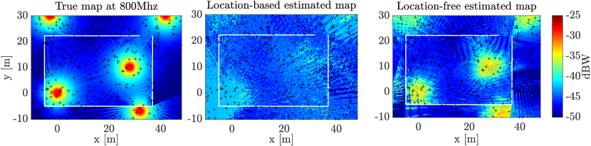
Figure 5: (left) True map, (middle) LocB (${{\color[rgb]{0,0,0}\lambda}}^{\prime}=3.3\times 10^{-3}$, $\sigma^{\prime}=0.5$ m), and (right) LocF (${{\color[rgb]{0,0,0}\lambda}}=1.9\times 10^{-4}$, $\sigma=37$ m) estimated maps; $N=300$, ${{\color[rgb]{0,0,0}L}}=5$, $B=20$ MHz, and $K=10$. The black crosses indicate the sensor locations and the solid white lines represent the walls of the building.

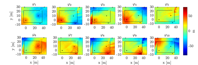
Figure 6: Maps of the ${{\color[rgb]{0,0,0}M}}=10$ LocF features with ${{\color[rgb]{0,0,0}L}}=5$, $B=20$ MHz, and $K=10$. The solid black lines represent the walls of the building and the black stars represent the transmitter locations.

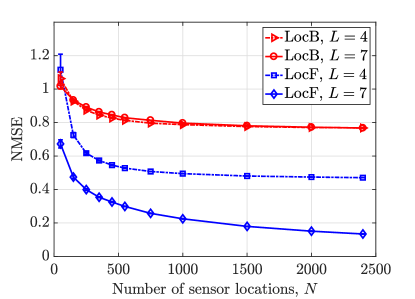
Figure 7: Performance comparison between the LocF cartography (${{\color[rgb]{0,0,0}\lambda}}=1.9\times 10^{-4}$, $\sigma=37$ m) and the LocB cartography (${{\color[rgb]{0,0,0}\lambda}}^{\prime}=3.3\times 10^{-3}$, $\sigma^{\prime}=0.5$ m) with $B=20$ MHz and $K=10$.

This section evaluates the performance of LocF cartography in presence of multipath, where localization algorithms cannot achieve accurate location estimates. To this end, the simulations are carried out in a 42 $\times$ 27 m structure comprising several parallel vertical planes modeling the external and internal walls of a building, the latter is located in a 60 $\times$ 40 m rectangular area $\mathcal{X}$. This area contains ${{\color[rgb]{0,0,0}L}}$ active transmitters. Some of these are positioned inside the building, others outside. Matrix ${\color[rgb]{0,0,0}\bm{Y}}_{n}\in\mathbb{C}^{{{\color[rgb]{0,0,0}L}}\times K}$ containing the noisy received pilot signals is generated according to (10), where $K$ is adjusted depending on $B$ to capture all the multipath components. For simplicity, the pilot signals are given by ${{\color[rgb]{0,0,0}a}}_{{\color[rgb]{0,0,0}l}}[k]=\delta[k]$ which implies that the rows of ${\color[rgb]{0,0,0}\bm{Y}}_{n}\in\mathbb{C}^{{{\color[rgb]{0,0,0}L}}\times K}$ contain the impulse responses of the bandlimited channels between the ${{\color[rgb]{0,0,0}L}}$ transmitters and the $n$-th measurement location. The channel $h_{{{\color[rgb]{0,0,0}l}},n}[k]$ is generated following (12) with a carrier frequency of 800 MHz and pilot channel bandwidth $B=1/T$. The noise samples ${{\color[rgb]{0,0,0}w}}_{{{\color[rgb]{0,0,0}l}},n}[k]$ are independent normal random variables with zero-mean and variance -70 dBm.

TABLE I: Parameters used for the experiment in Fig. 8.

	$B$ (MHz)	$50$	$100$	$200$	$700$
	$K$	$25$	$50$	$100$	$350$
LocB	$\sigma^{\prime}$ (m)	$10.1$	$8.9$	$9$	$7$
	${{\color[rgb]{0,0,0}\lambda}}^{\prime}$	$1.8\times 10^{-3}$	$9.1\times 10^{-4}$	$7.1\times 10^{-4}$	$2.1\times 10^{-4}$
LocF	$\sigma$ (m)	$27$	$41$	$53$	$28$
	${{\color[rgb]{0,0,0}\lambda}}$	$3.81\times 10^{-4}$	$6.1\times 10^{-5}$	$1.1\times 10^{-5}$	$5\times 10^{-4}$

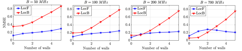
Figure 8: LocF and LocB map NMSE as a function of the number of walls for different values of the bandwidth, ${{\color[rgb]{0,0,0}L}}=5$, $N=300$.

Propagation adheres to the Motley-Keenan multi-wall radio propagation model [46], which accounts for the direct path, up to 5 first-order wall reflections, and up to 5 wall-to-wall second-order reflections. Remarkably, the model captures the impact of the angle of incidence on the power of the reflected ray. For simplicity, the C2M is chosen to be the channel where localization pilot signals are transmitted. In practice, this is the case in the downlink of a cellular communication system such as LTE where the base stations transmit both communication signals and localization pilots.

To ensure that the measurements are obtained in the far-field propagation region, sensor locations are spread uniformly at random over $\bar{\mathcal{X}}$, which comprises those points in $\mathcal{X}$ lying at least 3 wavelengths away from all transmitters. Note that, although the number of sensor locations is sometimes in the order of hundreds, this does not mean that a large number of sensing devices must be used since each device may gather measurements at tens or hundreds of spatial locations. The power measurement ${p}_{n}$ (measured in dBW) of the C2M at position $\bm{x}_{n}$ is corrupted by additive noise $\epsilon_{n}$ to yield $\tilde{p}_{n}=p_{n}+\epsilon_{n}$, where $\{\epsilon_{n}\}_{n=1}^{N}$ are independent normal random variables with zero-mean and variance $\sigma_{\epsilon}^{2}$. This variance is such that the signal-to-noise ratio defined as $10\log_{10}(\bar{p}^{2}/\sigma_{\epsilon}^{2})\approx 40$ dB, where $\bar{p}:=\int_{\bar{\mathcal{X}}}p(\bm{x})d\bm{x}/\int_{\bar{\mathcal{X}}}d\bm{x}$ is the spatial average of $p(\bm{x})$. This SNR is considered practical since the measurement noise power $\sigma_{\epsilon}^{2}$ can be driven arbitrarily close to zero in practice by averaging over a sufficiently long time window.

Quantitative evaluation will compare the normalized mean square error (NMSE) defined as:

$$\text{NMSE}=\frac{\mathbb{E}\{|p(\bm{x})-\hat{p}_{{\color[rgb]{0,0,0}\bm{Y}}}(\bm{Y}(\bm{x}),\mathcal{T})|^{2}\}}{\mathbb{E}\{|p(\bm{x})-\bar{p}|^{2}\}},$$ (28)

where $\hat{p}_{{\color[rgb]{0,0,0}\bm{Y}}}(\bm{Y}(\bm{x}),\mathcal{T})$ (measured in dBW) denotes the result of evaluating the map constructed from the training set $\mathcal{T}:=\{(\bm{Y}_{n},\tilde{p}_{n})\}_{n=1}^{N}$ at the location $\bm{x}$, where ${\color[rgb]{0,0,0}\bm{Y}}(\bm{x})$ comprises the received pilot signals at $\bm{x}$. The denominator in (28) normalizes the square error of the considered algorithm by the error incurred by the best data-agnostic estimator, which estimates the spatial average $\bar{p}$ at all points. Thus, the adopted performance metric is higher than traditional NMSE, meaning that it is more challenging to obtain lower values. Furthermore $\mathbb{E}\{\cdot\}$ denotes the expectation over the sensor locations and noise.

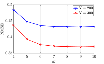
Figure 9: LocF estimated map NMSE for different values of number of features ${{\color[rgb]{0,0,0}M}}$ and sensor locations $N$, with ${{\color[rgb]{0,0,0}L}}=5$, $B=20$ MHz, $K=10$, ${{\color[rgb]{0,0,0}\lambda}}=1.9\times 10^{-4}$, and $\sigma=37$ m.

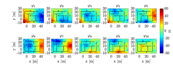
(a)

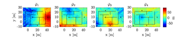
(b)

Figure 10: Maps of: (a) all the ${{\color[rgb]{0,0,0}M}}=10$ features and (b) ${{{\color[rgb]{0,0,0}r}}}=4$ reduced features with ${{\color[rgb]{0,0,0}L}}=5$, $B=20$ MHz, and $K=10$. The solid black lines represent the walls of the building and the black stars represent the transmitter locations. The maps are obtained by representing the value of the feature at every location in $\mathcal{X}$.

V-A LocF vs. LocB

To avoid the need for synchronization between transmitters and sensors, the LocF algorithm utilizes the features in (17), which additionally provide robustness to multipath and evolve smoothly over space; see Sec. IV-A. Since this center of mass can be thought of as a lag, it is scaled by the sampling period $T$ and speed of light $c$ to obtain the corresponding range difference, i.e.:

$$\begin{split}{\color[rgb]{0,0,0}\bm{\phi}}_{n}:=Tc~{}&[{\color[rgb]{0,0,0}\text{CoM}}_{1,2,n},{\color[rgb]{0,0,0}\text{CoM}}_{1,3,n},\ldots,{\color[rgb]{0,0,0}\text{CoM}}_{1,{{\color[rgb]{0,0,0}L}},n},\\ &{\color[rgb]{0,0,0}\text{CoM}}_{2,3,n},\ldots,{\color[rgb]{0,0,0}\text{CoM}}_{{{\color[rgb]{0,0,0}L}}-1,{{\color[rgb]{0,0,0}L}},n}]^{\top}.\end{split}$$ (29)

Using these features, the LocF algorithm uses the kernel ridge regression technique in Sec. III-B with Gaussian radial basis functions with parameter $\sigma$. The reason is that this universal kernel is capable of approximating arbitrary continuous functions that vanish at infinity [47]. On the other hand, for LocB cartography, the feature vector ${\color[rgb]{0,0,0}\bm{\phi}}_{n}={\hat{\bm{x}}}_{n}\in\mathbb{R}^{2}$ comprises estimates of the spatial coordinates of the $n$-th sensor location obtained by the iterative re-weighting squared range difference-least squares (IRWSRD-LS) algorithm [48], which features state-of-the-art localization performance. This algorithm is applied over TDoA features extracted from $\{{{\color[rgb]{0,0,0}\bm{Y}}}_{n}\}_{n=1}^{N}$ through (16). At the $n$-th sensor location, these features $\{\hat{{{\color[rgb]{0,0,0}\Delta}}}_{1,{{\color[rgb]{0,0,0}l}}^{\prime},n}\}_{{{\color[rgb]{0,0,0}l}}^{\prime}=2}^{{{\color[rgb]{0,0,0}L}}}$ comprise the TDoA between a reference base station and the remaining ${{\color[rgb]{0,0,0}L}}-1$ base stations. Enlarging this set by including TDoA measurements $\hat{{{\color[rgb]{0,0,0}\Delta}}}_{{{\color[rgb]{0,0,0}l}},{{\color[rgb]{0,0,0}l}}^{\prime},n}$ with ${{\color[rgb]{0,0,0}l}}\neq 1$ would not be beneficial for the estimation performance as discussed in [49]. The reason is the redundancy inherent to TDoA features described in Sec. IV-B. To ensure a fair comparison, LocB utilizes the same function learning algorithm as LocF; see Sec. III-B. Specifically, given $\left\{({\hat{\bm{x}}}_{n},\tilde{p}_{n})\right\}_{n=1}^{N}$, the map is estimated as $\hat{p}({\hat{\bm{x}}})=\bm{\kappa}^{\prime\top}({\hat{\bm{x}}}){\hat{\bm{\beta}}}$ where  $\bm{\kappa}^{\prime}({\hat{\bm{x}}}):=\left[\kappa^{\prime}({\hat{\bm{x}}},{\hat{\bm{x}}}_{1}),\ldots,\kappa^{\prime}({\hat{\bm{x}}},{\hat{\bm{x}}}_{N})\right]^{\top}$,  ${\hat{\bm{\beta}}}:=(\bm{K}^{\prime}+{{\color[rgb]{0,0,0}\lambda}}^{\prime}N\textbf{I}_{N})^{-1}\tilde{\bm{p}}$,  and $\bm{K}^{\prime}$ is an $N\times N$ matrix with $(n,n^{\prime})$-th entry $\kappa^{\prime}({\hat{\bm{x}}}_{n},{\hat{\bm{x}}}_{n^{\prime}})$ and $\kappa^{\prime}$ is a Gaussian radial basis function with parameter $\sigma^{\prime}$. In this way, this benchmark LocB algorithm coincides with those in [5, 14] when a power map must be estimated on a single frequency and with a single kernel. In all experiments, the values of ${{\color[rgb]{0,0,0}\lambda}}$, ${{\color[rgb]{0,0,0}\lambda}}^{\prime}$, $\sigma$, and $\sigma^{\prime}$ used by the LocF and LocB schemes were tuned to approximately yield the lowest NMSE.

Fig. 5 (left) depicts the true map generated through the multi-wall model, where the black crosses indicate the sensor locations and the solid white lines represent the walls of the building. The middle and right panels respectively show the LocB and LocF map estimates, obtained by placing a query sensor at every location. It is observed that the quality of the LocF estimate is considerably higher than that of the LocB estimate. The cause for the poor perfomance of the LocB algorithm is that the location estimates evolve in a non-smooth fashion across space, and attempting to learn the C2M from such non-smooth features is more challenging; see Figs. 1c and 1d and the discussion in Sec. I. To illustrate how the LocF approach alleviates this issue, Fig. 6 depicts the features used by the LocF estimator across $\mathcal{X}$. Specifically, if ${\color[rgb]{0,0,0}\bm{\phi}}(\bm{x})$ denotes the feature vector, obtained as in (29) for location $\bm{x}$, then the ${{\color[rgb]{0,0,0}m}}$-th panel titled $\varphi_{{\color[rgb]{0,0,0}m}}$ in Fig. 6 corresponds to the ${{\color[rgb]{0,0,0}m}}$-th entry of ${\color[rgb]{0,0,0}\bm{\phi}}(\bm{x})$ for each $\bm{x}\in\mathcal{X}$. It is observed that the evolution of these proposed features across space is significantly smoother than the one in Figs. 1c and 1d. A quantitative comparison is provided in Fig. 7, which shows the NMSE as a function of the number of sensor locations $N$ for ${{\color[rgb]{0,0,0}L}}=4$ and $7$ transmitters. The error bars delimit intervals of 6 standard deviations of the NMSE across the 200 independent Monte Carlo runs. It is observed that, with high significance, the proposed LocF cartography scheme outperforms its LocB counterpart for both values of ${{\color[rgb]{0,0,0}L}}$ provided that the number of measurement locations is roughly larger than 150.

The rest of the section studies the impact of multipath on the LocF and LocB cartography approaches by varying the number of walls. Fig. 8 shows the NMSE as a function of the number of walls for different values of $B$. The parameters used for both LocF and LocB schemes are listed in Table I. The NMSE is obtained by also averaging over wall locations, which are confined to be in the positions of the walls in Fig. 6 plus an additional wall that divides the room in two.

As expected, for all the simulated values of $B$, the performance of both LocF and LocB schemes is degraded (yet more severely in LocB) as the number of walls increases. Moreover, the performance of the LocB improves significantly with the bandwidth, since a higher bandwidth allows a more accurate estimation of the TDoA. This is because multipath components arriving within a time interval of length $T=1/B$ cannot be resolved; see Sec. IV-A and references therein. As intuition predicts, when multipath is sufficiently low and the bandwidth is sufficiently high, LocB cartography outperforms LocF. It is remarkable that LocF cartography exhibits robustness to multipath since the NMSE remains approximately constant even for a significant increase of multipath.

V-B Feature Design

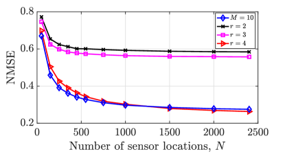
Figure 11: Estimated map NMSE with reduced features for different ${{{\color[rgb]{0,0,0}r}}}$ and without reduced features; ${{\color[rgb]{0,0,0}L}}=5$, $B=20$ MHz, $K=10$, ${{\color[rgb]{0,0,0}\lambda}}=1.6\times 10^{-3}$, and $\sigma=25$ m.

This section provides empirical support for the findings in Sec. IV-B. From now on, all experiments will involve only the LocF estimator. The first experiment investigates the impact of the number of features, which in all previous simulations was equal to ${{\color[rgb]{0,0,0}M}}={{\color[rgb]{0,0,0}L}}({{\color[rgb]{0,0,0}L}}-1)/2$. To this end, Fig. 9 shows the NMSE as a function of the number ${{\color[rgb]{0,0,0}M}}$ of features for two different numbers $N$ of sensor locations. The expectation operators in (28) also average with respect to all choices of ${{\color[rgb]{0,0,0}M}}$ features out of the ${{{\color[rgb]{0,0,0}L}}({{\color[rgb]{0,0,0}L}}-1)/2}$. As observed, the NMSE improves from ${{\color[rgb]{0,0,0}M}}=4$ to roughly ${{\color[rgb]{0,0,0}M}}=7$ features, and remains approximately the same for ${{\color[rgb]{0,0,0}M}}\geq 7$. Although this effect may look counter-intuitive at first glance, this is a common phenomenon in machine learning related to the bias-variance trade-off [33] and the curse of dimensionality [32, 33]; see Sec. III-A. Clearly, this effect motivates the feature dimensionality reduction techniques proposed in Sec. IV-B. The rest of this section corroborates the merits of such techniques. A more challenging scenario with more walls will be considered. The first step is to determine the number of reduced features to be used. It can be seen that ${{{\color[rgb]{0,0,0}r}}}=4$ in (21) retains at least ${{\color[rgb]{0,0,0}\eta}}=99\%$ of the variance of the features in all tested scenarios. Thus, in principle, a map can be learned using the reduced features ${{\color[rgb]{0,0,0}{\bar{\bm{\phi}}}}}_{n}:=\bm{U}_{1}^{\top}{\color[rgb]{0,0,0}\bm{\phi}}_{n}\in\mathbb{R}^{4}$ without meaningfully sacrificing estimation performance. Before corroborating that this is actually the case, it is instructive to visualize the aforementioned reduced features across space. Fig. 10a portrays the maps of the ${{\color[rgb]{0,0,0}M}}=10$ original features, which correspond to the entries of ${\color[rgb]{0,0,0}\bm{\phi}}(\bm{x})$; see Sec. V-A. On the other hand, the panels of Fig. 10b depict the reduced features over space, i.e., the 4 entries of the vector ${{\color[rgb]{0,0,0}{\bar{\bm{\phi}}}}}(\bm{x}):=\bm{U}_{1}^{\top}{\color[rgb]{0,0,0}\bm{\phi}}(\bm{x})$ for each $\bm{x}\in\mathcal{X}$. These figures reveal that the reduced features inherit the spatial smoothness of the original features.

To quantify the impact of reducing the dimensionality of the feature vectors, Fig. 11 compares the NMSE of the LocF map estimate that relies on the original features (${{\color[rgb]{0,0,0}M}}=10$) with the one that relies on the reduced features (${{\color[rgb]{0,0,0}r}}=2,3,4$). As observed, using just the 4 reduced features attains a similar performance to the estimator built on the 10 original features. This is expected given the bias-variance trade-off mentioned earlier. At this point, it might seem that the effects observed in Fig. 9 contradict those of Fig. 11 since in the former the NMSE is lower when 10 features are used relative to the case where only 4 are used. However, that should not be concluded since the features in Fig. 9 correspond to the entries of ${\color[rgb]{0,0,0}\bm{\phi}}_{n}$ (see (29)) whereas the features in Fig. 11 correspond to the entries of ${{\color[rgb]{0,0,0}{\bar{\bm{\phi}}}}}_{n}:=\bm{U}_{1}^{\top}{\color[rgb]{0,0,0}\bm{\phi}}_{n}$.

V-C LocF cartography with Missing Features

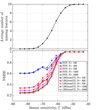
Figure 12: (top) Average number of missing features and (bottom) estimated map NMSE, both as a function of ${{\color[rgb]{0,0,0}\Gamma}}$ with ${{\color[rgb]{0,0,0}L}}=5$, $B=20$ MHz, $K=10$, ${{\color[rgb]{0,0,0}\lambda}}=1.9\times 10^{-4}$, ${{\color[rgb]{0,0,0}\mu}}=5.42$, and $\sigma=37$ m.

This section assesses the performance of the techniques developed in Sec. IV-C to cope with missing features.

A feature will be deemed missing at a given sensor location if the received power of at least one of the two associated pilot signals is below a sensitivity threshold ${{\color[rgb]{0,0,0}\Gamma}}$. The top panel of Fig. 12 depicts the average number of missing features as a function of ${{\color[rgb]{0,0,0}\Gamma}}$. The average is taken with respect to the sensor locations and noise. The bottom panel of Fig. 12 shows the LocF map NMSE also as a function of ${{\color[rgb]{0,0,0}\Gamma}}$. The matrix completion problem in (24) is solved with both SVP and LRGeomCG; the implementation for the latter is the one provided in the ManOpt toolbox [50]. For higher values of $N$, the performance of both algorithms is clearly strongly determined by the average number of missing features. SVP seems to outperform LRGeomCG in terms of NMSE. Besides, the computation time of SVP is roughly half the one of LRGeomCG.

VI Conclusions

Location-free (LocF) cartography has been proposed as an alternative to classical location-based (LocB) schemes, which suffer a strong performance degradation when multipath impairs the propagation of localization pilot signals. The central idea is to learn a map as a function of certain features of the localization pilot signals. Building upon this approach, kernel-ridge regression was applied to estimate power maps from these features. Practical issues addressed in the paper include feature design, dimensionality reduction, and dealing with missing features. Simulations corroborate the merits of LocF cartography relative to LocB alternatives. Future research will include mapping other channel metrics such as power spectral density (PSD) and channel gain, as well as developing distributed and online extensions.

References

- [1] Y. Teganya, L. M. Lopez-Ramos, D. Romero, and B. Beferull-Lozano, “Localization-free power cartography,” in Proc. IEEE Int. Conf. Acoust., Speech, Sig. Process., Calgary, Canada, Apr. 2018, pp. 3549–3553.
- [2] A. Alaya-Feki, S. B. Jemaa, B. Sayrac, P. Houze, and E. Moulines, “Informed spectrum usage in cognitive radio networks: Interference cartography,” in Proc. IEEE Int. Symp. Personal, Indoor Mobile Radio Commun., Cannes, France, Sep. 2008, pp. 1–5.
- [3] J.-A. Bazerque and G. B. Giannakis, “Distributed spectrum sensing for cognitive radio networks by exploiting sparsity,” IEEE Trans. Sig. Process., vol. 58, no. 3, pp. 1847–1862, Mar. 2010.
- [4] B. A. Jayawickrama, E. Dutkiewicz, I. Oppermann, G. Fang, and J. Ding, “Improved performance of spectrum cartography based on compressive sensing in cognitive radio networks,” in Proc. IEEE Int. Commun. Conf., Budapest, Hungary, Jun. 2013, pp. 5657–5661.
- [5] D. Romero, S-J. Kim, G. B. Giannakis, and R. López-Valcarce, “Learning power spectrum maps from quantized power measurements,” IEEE Trans. Sig. Process., vol. 65, no. 10, pp. 2547–2560, May 2017.
- [6] S. Grimoud, S. B. Jemaa, B. Sayrac, and E. Moulines, “A REM enabled soft frequency reuse scheme,” in Proc. IEEE Global Commun. Conf., Miami, FL, Dec. 2010, pp. 819–823.
- [7] E. Dall’Anese, S.-J. Kim, G. B. Giannakis, and S. Pupolin, “Power control for cognitive radio networks under channel uncertainty,” IEEE Trans. Wireless Commun., vol. 10, no. 10, pp. 3541–3551, Aug. 2011.
- [8] W.C.M.V. Beers and J.P.C. Kleijnen, “Kriging interpolation in simulation: A survey,” in Proc. IEEE Winter Simulation Conf., Washington, D. C., Dec. 2004, vol. 1, pp. 113–121.
- [9] G. Boccolini, G. Hernandez-Penaloza, and B. Beferull-Lozano, “Wireless sensor network for spectrum cartography based on kriging interpolation,” in Proc. IEEE Int. Symp. Personal, Indoor Mobile Radio Commun., Sydney, NSW, Nov. 2012, pp. 1565–1570.
- [10] G. Ding, J. Wang, Q. Wu, Y.-D. Yao, F. Song, and T. A Tsiftsis, “Cellular-base-station-assisted device-to-device communications in TV white space,” IEEE J. Sel. Areas Commun., vol. 34, no. 1, pp. 107–121, Jul. 2016.
- [11] S.-J. Kim, N. Jain, G. B. Giannakis, and P. Forero, “Joint link learning and cognitive radio sensing,” in Proc. Asilomar Conf. Sig., Syst., Comput., Pacific Grove, CA, Nov. 2011, pp. 1415 –1419.
- [12] S.-J. Kim and G. B. Giannakis, “Cognitive radio spectrum prediction using dictionary learning,” in Proc. IEEE Global Commun. Conf., Atlanta, GA, Dec. 2013, pp. 3206 – 3211.
- [13] D.-H. Huang, S.-H. Wu, W.-R. Wu, and P.-H. Wang, “Cooperative radio source positioning and power map reconstruction: A sparse Bayesian learning approach,” IEEE Trans. Veh. Technol., vol. 64, no. 6, pp. 2318–2332, Aug. 2014.
- [14] J.-A. Bazerque and G. B. Giannakis, “Nonparametric basis pursuit via kernel-based learning,” IEEE Sig. Process. Mag., vol. 28, no. 30, pp. 112–125, Jul. 2013.
- [15] M. Hamid and B. Beferull-Lozano, “Non-parametric spectrum cartography using adaptive radial basis functions,” in Proc. IEEE Int. Conf. Acoust., Speech, Sig. Process., New Orleans, LA, Mar. 2017, pp. 3599–3603.
- [16] J.-A. Bazerque, G. Mateos, and G. B. Giannakis, “Group-lasso on splines for spectrum cartography,” IEEE Trans. Sig. Process., vol. 59, no. 10, pp. 4648–4663, Oct. 2011.
- [17] S.-J. Kim, E. Dall’Anese, and G. B. Giannakis, “Cooperative spectrum sensing for cognitive radios using Kriged Kalman filtering,” IEEE J. Sel. Topics Sig. Process., vol. 5, no. 1, pp. 24–36, Jun. 2010.
- [18] D. Romero, D. Lee, and G. B. Giannakis, “Blind channel gain cartography,” in Proc. Global Conf. Sig. Inf. Process., Greater Washington, D. C., Dec. 2016, pp. 1110–1115.
- [19] D. Lee, S.-J. Kim, and G. B. Giannakis, “Channel gain cartography for cognitive radios leveraging low rank and sparsity,” IEEE Trans. Wireless Commun., vol. 16, no. 9, pp. 5953–5966, Jun. 2017.
- [20] D. Lee, D. Berberidis, and G. B. Giannakis, “Adaptive Bayesian channel gain cartography,” in Proc. IEEE Int. Conf. Acoust., Speech, Sig. Process., Calgary, Canada, Apr. 2018, pp. 3555–3558.
- [21] M. Bshara, U. Orguner, F. Gustafsson, and L. Van Biesen, “Fingerprinting localization in wireless networks based on received-signal-strength measurements: A case study on WiMAX networks,” IEEE Trans. Veh. Technol., vol. 59, no. 1, pp. 283–294, Aug. 2009.
- [22] P. S. Naidu, Distributed Sensor Arrays: Localization, CRC Press, 2017.
- [23] A. Bensky, Wireless Positioning Technologies and Applications, Artech House, 2016.
- [24] H. Liu, H. Darabi, P. Banerjee, and J. Liu, “Survey of wireless indoor positioning techniques and systems,” IEEE Trans. Syst., Man, Cybernetics C., Appl. Rev., vol. 37, no. 6, pp. 1067–1080, Nov. 2007.
- [25] InfSoft, “Ultra-wideband,” [Online]. Available: https://www.ultrawideband.io/en/technology.php.
- [26] L. Yang and G. B. Giannakis, “Ultra-wideband communications: An idea whose time has come,” IEEE Sig. Process. Mag., vol. 21, no. 6, pp. 26–54, Nov. 2004.
- [27] D. Dardari, C.-C. Chong, and M. Win, “Threshold-based time-of-arrival estimators in UWB dense multipath channels,” IEEE Trans. Commun., vol. 56, no. 8, pp. 1366–1378, Aug. 2008.
- [28] M. Brunato and R. Battiti, “Statistical learning theory for location fingerprinting in wireless LANs,” Computer Networks, vol. 47, no. 6, pp. 825–845, Apr. 2005.
- [29] P. Prasithsangaree, P. Krishnamurthy, and P. K. Chrysanthis, “On indoor position location with wireless LANs,” in Proc. IEEE Int. Symp. Personal, Indoor Mobile Radio Commun., Lisboa, Portugal, Sep. 2002, vol. 2, pp. 720–724.
- [30] HP, “SmartLOCUS,” [Online]. Available: https://www.rfidjournal.com.
- [31] L. M. Ni, Y. Liu, Y. C. Lau, and A. P. Patil, “LANDMARC: Indoor location sensing using active RFID,” in Proc. IEEE Int. Conf. Pervasive Computing Commun., Fort Worth, TX, Mar. 2003, pp. 407–415.
- [32] C. M. Bishop, Pattern Recognition and Machine Learning, Information Science and Statistics. Springer, 2006.
- [33] V. Cherkassky and F. M. Mulier, Learning from Data: Concepts, Theory, and Methods, John Wiley & Sons, 2007.
- [34] B. Schölkopf and A. J. Smola, Learning with Kernels: Support Vector Machines, Regularization, Optimization, and Beyond, MIT Press, 2002.
- [35] B. Schölkopf, R. Herbrich, and A. J. Smola, “A generalized representer theorem,” in Proc. Comput. Learning Theory, Amsterdam, The Netherlands, Jul. 2001, pp. 416–426.
- [36] A. Goldsmith, Wireless Communications, Cambridge University Press, 2005.
- [37] S. W. Smith, The Scientist and Engineer’s Guide to Digital Signal Processing, California Technical Publishing, 1997.
- [38] N. E. Gemayel, S. Koslowski, F. K. Jondral, and J. Tschan, “A low cost TDOA localization system: Setup, challenges and results,” in Proc. Workshop Pos. Navigation Commun., Dresden, Germany, Mar. 2013, pp. 1–4.
- [39] M. Fazel, Matrix Rank Minimization with Applications, Ph.D. thesis, Stanford University, 2002.
- [40] E. J. Candès and B. Recht, “Exact matrix completion via convex optimization,” Foundations Comput. Math., vol. 9, no. 6, pp. 717–772, Apr. 2009.
- [41] B. Recht, M. Fazel, and P. A. Parrilo, “Guaranteed minimum-rank solutions of linear matrix equations via nuclear norm minimization,” SIAM J. Opt., vol. 52, no. 3, pp. 471–501, Aug. 2010.
- [42] E. J. Candès and T. Tao, “The power of convex relaxation: Near-optimal matrix completion,” IEEE Trans. Inf. Theory, vol. 56, no. 5, pp. 2053–2080, Apr. 2010.
- [43] P.-A. Absil, R. Mahony, and R. Sepulchre, Optimization Algorithms on Matrix Manifolds, Princeton University Press, 2009.
- [44] B. Vandereycken, “Low-rank matrix completion by riemannian optimization,” SIAM J. Opt., vol. 23, no. 2, pp. 1214–1236, Jun. 2013.
- [45] P. Jain, R. Meka, and I. S. Dhillon, “Guaranteed rank minimization via singular value projection,” in Proc. Advances in Neural Inf. Proces. Syst., Vancouver, Canada, Dec. 2010, pp. 937–945.
- [46] S. Hosseinzadeh, H. Larijani, and K. Curtis, “An enhanced modified multi wall propagation model,” in Proc. IEEE Global Internet of Things Summit, Geneva, Switzerland, Jun. 2017, pp. 1–4.
- [47] C. A. Micchelli, Y. Xu, and H. Zhang, “Universal kernels,” J. Mach. Learn. Res., vol. 7, pp. 2651–2667, Dec. 2006.
- [48] D. Ismailova and W.-S. Lu, “Improved least-squares methods for source localization: An iterative re-weighting approach,” in Proc. IEEE Int. Conf. Dig. Sig. Process., Singapore, Jul. 2015, pp. 665–669.
- [49] R. Kaune, “Accuracy studies for TDOA and TOA localization,” in Proc. IEEE Int. Conf. Inf. Fusion, Singapore, Jul. 2012, pp. 408–415.
- [50] N. Boumal, B. Mishra, P-A. Absil, and R. Sepulchre, “ManOpt, a MATLAB toolbox for optimization on manifolds,” J. Mach. Learn. Res., vol. 15, no. 1, pp. 1455–1459, Apr. 2014.