Accelerated Consensus for Multi-Agent Networks
through Delayed Self Reinforcement

Abstract

This article aims to improve the performance of networked multi-agent systems, which are common representations of cyber-physical systems. The rate of convergence to consensus of multi-agent networks is critical to ensure cohesive, rapid response to external stimuli. The challenge is that increasing the rate of convergence can require changes in the network connectivity, which might not be always feasible. Note that current consensus-seeking control laws can be considered as a gradient-based search over the graph’s Laplacian potential. The main contribution of this article is to improve the convergence to consensus, by using an accelerated gradient-based search approach. Additionally, this work shows that the accelerated-consensus approach can be implemented in a distributed manner, where each agent applies a delayed self reinforcement, without the need for additional network information or changes to the network connectivity. Simulation result shows that the convergence rate with the accelerated consensus is about double the convergence rate of current consensus laws. Moreover, the loss of synchronization during the transition is reduced by about ten times with the use of the proposed accelerated-consensus approach.

I Introduction

Multi-agent networks are common cyber-physical systems with applications such as autonomous vehicles, swarms of robots and other unmanned systems, e.g.,  [1, 2, 3, 4, 5, 6, 7, 8]. The performance of such systems, such as the response to external stimuli, depends on rapidly transitioning from one operating point (consensus value) to another, e.g., as seen in flocking, [9, 10]. Thus, there is interest to increase the convergence to consensus for such networked multi-agent systems.

A challenge is that there are fundamental limits to the achievable convergence to consensus using existing graph-based update laws for a given network, e.g., of the form

$$Z[k+1]=\left[{\textbf{I}}-\gamma K\right]Z(k)=PZ[k]$$ (1)

where the current state is $Z(k)$, the updated state is $Z[k+1]$, $\gamma$ is the update gain, $K$ is the graph Laplacian and $P$ is the Perron matrix. Hence the convergence to consensus depends on the eigenvalues of the Perron matrix $P$, which in turn depends on the eigenvalues of the graph Laplacian $K$. For example, if the underlying graph is undirected and connected, it is well known that convergence to consensus can be achieved provided the update gain $\gamma$ is sufficiently small, e.g., [11]. The gain $\gamma$ can be selected to maximize the convergence rate. However, for a given graph (i.e., a given graph Laplacian $K$), the range of the acceptable update gain $\gamma$ is limited, which in turn, limits the achievable rate of convergence as shown in previous work [12]. Although it is possible to change the convergence by choosing the Perron matrix [13], i.e., by choosing a different graph structure for the network, the maximum rate of convergence with current graph-based updates is bounded for a given network structure.

As discussed in [12], current limitations in graph-based approaches motivate the development of new approaches to improve the convergence to consensus. Note that the convergence can be slow if the number of agent inter-connections is small compared to the number of agents, e.g., [14]. Randomized time-varying connections can lead to faster convergence, as shown in, e.g., [14]. The update sequence of the agents can also be arranged to improve convergence, e.g., [15]. When such time-variations in the graph structure or selection of the graph Laplacian $K$ are not feasible, the need to maintain stability limits the range of acceptable update gain $\gamma$, and therefore, limits the rate of convergence. This convergence-rate limitation motivates the proposed effort to develop a new approach to improve the network performance.

The major contribution of this work is to use an accelerated-gradient-based approach to modify the standard update law in Eq. (1) for networked multi-agent systems. Previous works have used such acceleration methods (also referred to as the Nesterov’s gradient method) to improve the convergence of gradient-based search in learning algorithms, e.g., see  [16, 17]. Another contribution is to show that the proposed accelerated approach to consensus can be implemented by using a delayed self reinforcement (DSR), where each agent only uses current and past information from the network. This use of already existing information is advantageous since the consensus improvement is achieved without the need to change the network connectivity and without the need for additional information from the network. This work generalizes the author’s previous works in [12, 18, 19], which considered a momentum term only to improve the convergence to consensus.

Simulation results of an example networked system are presented in this work to show that the proposed accelerated-consensus approach with DSR can substantially improve synchronization during the transition by about ten times, in addition to decreasing the transition time by about half, when compared to the case without the DSR approach. This is shown to improve formation control during transitions in networked multi-agent systems.

II Problem formulation

II-A Background: network-based consensus control

Let the multi-agent network be modeled using a graph representation, where the connectivity of the agents is represented by a directed graph (digraph) ${\cal{G}}=\left({\cal{V}},{\cal{E}}\right)$, e.g., as defined in [11]. Here, the agents are represented by nodes ${\cal{V}}=\left\{1,2,\ldots,{n\!+\!1}\right\}$, $n>1$ and their connectivity by edges ${\cal{E}}\subseteq{\cal{V}}\times{\cal{V}}$, where each agent $j$ belonging to the set of neighbors $N_{i}\subseteq{\cal{V}}$ of the agent $i$ satisfies $j\neq i$ and $(j,i)\in{\cal{E}}$.

II-B Graph-based control

The consensus control for the multi-agent network is defined by the graph ${\cal{G}}$, as

$$\hat{Z}[k+1] =\hat{Z}[k]+\gamma u(k)$$

$$=\hat{Z}[k]+\gamma\sum_{i,j=1}^{n}a_{ij}\left(\hat{Z}_{j}[k]-\hat{Z}_{i}[k]\right)$$

$$=\hat{Z}[k]-\gamma L\hat{Z}[k]$$

$$=\left({\bf{I}}-\gamma L\right)\hat{Z}[k]$$ (2)

where $\hat{Z}$ represents the states of the agents, $k$ represents the time instants $t_{k}=k\delta_{t}$, $\gamma$ is the update gain, $u$ is the input to each agent, the weight $a_{i,j}$ is nonzero (and positive) if and only if $j$ is in the set of neighbors $N_{i}\subseteq{\cal{V}}$ of the agent $i$, and the terms $l_{ij}$ of the $(n+1)\times(n+1)$ Laplacian $L$ of the graph ${\cal{G}}$ are real and given by

$$l_{ij} =\left\{\begin{array}[]{ll}-a_{ij}<0,&{\mbox{if}}~{}j\in N_{i}\\ \sum_{m=1}^{n+1}a_{im},&{\mbox{if}}~{}j=i,\\ 0&{\mbox{otherwise,}}\end{array}\right.$$ (6)

where each row of the Laplacian $L$ adds to zero, i.e., from Eq. (6), the $(n+1)\times 1$ vector of ones ${\textbf{1}}_{n+1}=[1,\ldots,1]^{T}$ is a right eigenvector of the Laplacian $L$ with eigenvalue $0$,

$$L{\textbf{1}}_{n+1} =0{\textbf{1}}_{n+1}.$$ (7)

II-C Network dynamics

One of the agents is assumed to be a virtual source agent, which can be used to specify a desired consensus value $Z_{d}$. Without loss of generality, the last node, $n+1$ is assumed to be a virtual source agent. Moreover, each agent in the network should have access to the source agent’s state ${Z}_{s}=\hat{Z}_{n+1}$ through the network, as formalized below.

Assumption 1 (Connected graph)

The digraph ${\cal{G}}$ is assumed to have a directed path from the source node ${n+1}$ to any other node $i$ in the graph, i.e., $i\in{\cal{V}}\setminus\!{(n+1)}$. ∎

Some properties of the graph ${\cal{G}}$ without the source node $n+1$ are listed below, e.g., [11]. In particular, consider the $n\times n$ pinned Laplacian matrix $K$ obtained by removing the row and column associated with the source node $n+1$, the following partitioning of the Laplacian $L$ is invertible, i.e.,

$$L =\left[\begin{array}[]{c|c}K&-B\\ \hline\cr\star_{1\times n}&\star_{1\times 1}\end{array}\right]~{}\quad{\mbox{with}}~{}~{}\det{(K)}\neq 0,$$ (10)

and $B$ is an $n\times 1$ matrix

$$\begin{array}[]{rl}B&=[a_{1,s},a_{2,s},\ldots,a_{n,s}]^{T}\\ &~{}=[B_{1},B_{2},\ldots,B_{n}]^{T},\end{array}$$ (11)

Non-zero values of $B_{j}$ implies that the agent $j$ is directly connected to the source $Z_{s}$.

1. The pinned Laplacian matrix $K$ is invertible from the Assumption 1 and the Matrix-Tree Theorem in [20].

2. The eigenvalues of $K$ have have strictly-positive, real parts.

3. The product of the inverse of the pinned Laplacian $K$ with $B$ leads to a $n\times 1$ vector of ones, i.e.,

   $$K^{-1}B ={\textbf{1}}_{n}.$$ (12)

The dynamics of the non-source agents $Z$ represented by the remaining graph ${\cal{G}}\!\setminus\!s$, be given by

$$\begin{array}[]{rl}Z[k+1]&=Z[k]-\gamma KZ[k]+\gamma BZ_{s}[k]\\ &=\left({\bf{I}}-\gamma K\right)Z[k]+\gamma BZ_{s}(k)\\ &=PZ[k]+\gamma BZ_{s}(k).\end{array}$$ (13)

where $P$ is Perron matrix.

A sufficiently small selection of the update gain $\gamma$ will stabilize the dynamics in Eq. (13), e.g., see [11], i.e., all eigenvalues $\lambda_{P,i}$ of the Perron matrix

$$P~{}={\textbf{I}}_{n\times n}-\gamma K,$$

where ${\textbf{1}}_{n\times n}$ is the $n\times n$ identity matrix, will lie inside the unit circle.

II-D Stable consensus

With a stabilizing update gain $\gamma$, the state $Z$ of the network (of all non-source agents) converges to a fixed source value $Z_{s}$, e.g., for a step change in the source value $Z_{s}$, i.e., $Z_{s}[k]=Z_{d}$ for $k>0$ and zero otherwise. Since the eigenvalues of $P$ are inside the unit circle, the solution to Eq. (13) for the step input converges

$$\left[Z[k+1]-Z[k]\right] =P^{k}\left[Z[1]-Z[0]\right]\rightarrow 0$$ (14)

as $k\rightarrow\infty$. Therefore, taking the limit as $k\rightarrow\infty$ in Eq. (13), and from invertibility of the pinned Laplacian $K$ from Eq. (10).

$$Z[k]\rightarrow K^{-1}BZ_{d}$$ (15)

as $k\rightarrow\infty$. Then, from Eq. (12), the state $Z[k]$ at the non-source agents reaches the desired state $Z_{d}$ as time step $k$ increases, i.e,

$$Z[k] \rightarrow{\textbf{1}}_{n}Z_{d}~{}~{}{\mbox{as}}~{}~{}k\rightarrow\infty.$$ (16)

Thus, the control law in Eq. (13) achieves consensus.

II-E Convergence-rate limit

For a given pinned Laplacian $K$, the range of the acceptable update gain $\gamma$ is limited, which in turn limits the achievable rate of convergence. If

$$\lambda_{K,m}=m_{K,m}e^{i\phi_{K,m}}$$

is an eigenvalue of the pinned Laplacian $K$ with a corresponding eigenvector $V_{K,m}$, i.e.,

$$KV_{K,m}~{} =\lambda_{K,m}V_{K,m},$$ (17)

then

$$\lambda_{P,m}=1-\gamma\lambda_{K,m}$$

is an eigenvalue of the Perron matrix $P$ for the same eigenvector $V_{K,m}$, since

$$PV_{K,m}~{}=\left[{\textbf{I}}_{n\times n}-\gamma K\right]V_{K,m}=(1-\gamma\lambda_{K,m})V_{K,m}.$$ (18)

Lemma 1 (Perron matrix properties)

The network dynamics in Eq. (13), is stable if and only if the update gain $\gamma$ satisfies

$$0~{}<\gamma~{} <\min_{1\leq i\leq n}2\frac{\cos{(\phi_{K,i})}}{m_{K,i}}=\overline{\gamma}~{}<~{}\infty.$$ (19)

Proof: See [12]. ∎

The model in Eq. (13) can be rewritten as

$$\begin{array}[]{rl}\frac{Z[k+1]-Z[k]}{\delta_{t}}&=-\frac{\gamma}{\delta_{t}}KZ[k]+\frac{\gamma}{\delta_{t}}BZ_{s}[k]\end{array}$$ (20)

where $\delta_{t}$ is the time between updates. For a sufficiently-small update time $\delta_{t}$ it can considered as the discrete version of the continuous-time dynamics

$$\begin{array}[]{rl}\dot{Z}(t)&=-\frac{\gamma}{\delta_{t}}KZ(t)+\frac{\gamma}{\delta_{t}}BZ_{s}(t).\end{array}$$ (21)

The eigenvalues of $\frac{\gamma}{\delta_{t}}K$ increase proportionally with $\gamma$ and inversely with update time interval $\delta_{t}$. Therefore, the settling time $T_{s}$ of the continuous time system decreases as the gain $\frac{\gamma}{\delta_{t}}$ increases. The sampling time $\delta_{t}$ is bounded from below based on the sensing-computing-actuation bandwidth of the agents in the network, and the gain $\gamma$ is limited by the network structure as in Lemma 1. Consequently, the smallest possible update time $\delta_{t}$ and the given network structure limit the fastest possible settling time for a given network.

II-F The settling-time improvement problem

The research problem addressed in this article is to reduce the settling time $T_{s}$ (from one consensus state to another) under step changes in the source value (i.e., improve convergence) where each agent can modify its update law

1. using only existing information from the network neighbors,

2. without changing the network structure (network connectivity $K$), and

3. without changing the update-time interval $\delta_{t}$, which limits the maximum gain $\gamma$.

III Proposed accelerated consensus aproach

III-A Graph’s Laplacian potential

For undirected graphs, the control law $u$ in Eq. (2) can be considered as a gradient-based search based on the graph’s Laplacian potential $\Phi_{{\cal{G}}}$ [21],

$$u(\hat{Z}) =-{\frac{1}{2}}\nabla\Phi_{{\cal{G}}}(\hat{Z}),$$ (22)

where [21, 22]

$$\Phi_{{\cal{G}}}(\hat{Z}) =\frac{1}{2}\sum_{i,j=1}^{n}a_{ij}\left(\hat{Z}_{j}-\hat{Z}_{i}\right)^{2}$$ (23)

results in

$$u(\hat{Z}) =-{\frac{1}{2}}\nabla\Phi_{{\cal{G}}}(\hat{Z})~{}=-L\hat{Z}.$$ (24)

This results in, from Eq. (2),

$$\hat{Z}[k+1] =\hat{Z}[k]-\gamma{\frac{1}{2}}\nabla\Phi_{{\cal{G}}}(\hat{Z})$$

$$=\hat{Z}[k]-\gamma L\hat{Z}[k]$$ (25)

III-B Accelerated gradient search

In general, the convergence of the gradient-based approach as in Eq. (22) can be improved using accelerated methods. In particular, applying the Nesterov modification [16, 17] of the traditional gradient-based method to Eq. (22) results in

$$u(\hat{Z}[k]) =-{\frac{1}{2}}\nabla\Phi_{{\cal{G}}}\left\{\hat{Z}[k]+\beta\left(\hat{Z}[k]-\hat{Z}[k-1]\right)\right\}$$

$$\qquad+\beta\left(\hat{Z}[k]-\hat{Z}[k-1]\right)$$

$$=-L\left\{\hat{Z}[k]+\beta\left(\hat{Z}[k]-\hat{Z}[k-1]\right)\right\}$$

$$\qquad+\beta\left(\hat{Z}[k]-\hat{Z}[k-1]\right).$$ (26)

This accelerated-gradient-based input results in the modification of the system Eq. (2) to

$$\hat{Z}[k+1] =\hat{Z}[k]-\gamma L\left(\hat{Z}[k]+\beta\left(\hat{Z}[k]-\hat{Z}[k-1]\right)\right)$$

$$\qquad+\gamma\beta\left(\hat{Z}[k]-\hat{Z}[k-1]\right).$$ (27)

Consequently, the dynamics of the non-source agents $Z$ represented by the remaining graph ${\cal{G}}\!\setminus\!s$ and given by Eq. (13), becomes

$$\begin{array}[]{rl}Z[k+1]&=Z[k]-\gamma K\left(Z[k]+\beta\left({Z}[k]-{Z}[k-1]\right)\right)\\ &\qquad+\beta\left({Z}[k]-{Z}[k-1]\right)+\gamma BZ_{s}[k].\end{array}$$ (28)

Remark 1

For directed graphs, the potential in Eq. (23) does not lead to the graph Laplacian [21, 22]. Instead, the graph potential (without the source node) can be directly considered as

$$\Phi_{{\cal{G}}\!\setminus\!s}({Z}) ={Z}^{T}K{Z}+BZ_{s},$$ (29)

and the application of the accelerated-gradient approach leads to the same Eq. (31). ∎

III-C Implementation using delayed self reinforcement

The above accelerated-gradient approach for multi-agent networks can be implemented without additional information from the network, or having to change the network connectivity. For an agent $i$, let $v_{i}$ be the information obtained from the network, i.e.,

$$\begin{array}[]{rl}v_{i}[k]&=\gamma K_{i}Z[k]\\ \end{array}$$ (30)

where $K_{i}$ is the $i^{th}$ row of the pinned Laplacian $K$. Then, the update of agent $Z_{i}$ is, from Eq. (27),

$$\begin{array}[]{rl}Z_{i}[k+1]&=Z_{i}[k]-\gamma K_{i}\left(Z[k]+\beta\left({Z}[k]-{Z}[k-1]\right)\right)\\ &\qquad+\beta\left({Z}_{i}[k]-{Z}_{i}[k-1]\right)+\gamma B_{i}Z_{s}[k]\\[3.61371pt] &=Z_{i}[k]-\left(v_{i}[k]+\beta(v_{i}[k]-v_{i}[k-1])\right)\\ &\qquad+\beta\left({Z}_{i}[k]-{Z}_{i}[k-1]\right)+\gamma B_{i}Z_{s}[k]\end{array}$$ (31)

where $B_{i}$ is the $i^{th}$ row of the source connectivity matrix $B$. The delayed self-reinforcement (DSR) approach, however, requires each agent to store a delayed versions $Z_{i}[k-1]$ and $v_{i}[k-1]$ of its current state $Z_{i}[k]$ and information $v_{i}[k]$ from the network, as illustrated in Fig. 1.   ∎

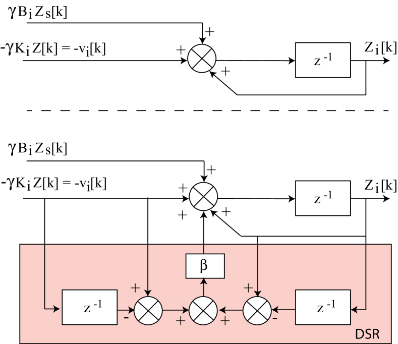
Figure 1: (Top) Implementation of standard gradient-based approach to multi-agent networks for the $i^{th}$ agent as in Eq. (13). (Bottom) Delayed self reinforcement (DSR) approach to implement the accelerated-gradient-based approach for the $i^{th}$ agent in Eq. (31) without using additional network information.

III-D Quantifying synchronization during transition

In general, it is not only important that the network reaches a new consensus value $Z_{d}$, but also that during the transition the network states are similar to each other. For example, consider the case when the state $Z$ of the agents are horizontal velocities $V_{x}$. Then having similar velocities during the transition (i.e., synchronization during the transition) can aid in maintaining the formation, without the need for additional control actions.

The lack of cohesion or synchronization during the transition can be quantified in terms of the deviation $\Delta$ in the response as

$$\Delta =\frac{\delta_{t}}{Z_{d}}\sum_{k=1}^{k_{Ts}}\left|Z[k]-\overline{Z}[k]\right|_{1}$$ (32)

where $k_{Ts}$ is the number of steps needed to reach the settling time $T_{s}$, which is time by which all agent responses $Z$ reach and stay within $2\%$ of the final value $Z_{d}$, $\overline{Z}$ is the average value of the state $Z$, over all individual agent state-components $z_{i}$, i.e.,

$$\overline{Z}[k] =\frac{1}{n}\sum_{i=1}^{n}Z_{i}[k],$$ (33)

and $|\cdot|_{1}$ is the standard vector 1-norm,

$$|\hat{Z}|_{1}=\sum_{i=1}^{n}|\hat{Z}_{i}|$$

for any vector $\hat{Z}$. A normalized measure ${\Delta}^{*}$ that removes the effect of the response speed is obtained by dividing the expression in Eq. (32) with the settling time $T_{s}$ as

$${\Delta}^{*} =\frac{\Delta}{T_{s}}.$$ (34)

Note that the system’s transient response is more synchronized if the normalized deviation ${\Delta}^{*}$ is small.

IV Results and discussion

The step response of an example system, with and without DSR, are comparatively evaluated. Moreover, the impact of using DSR on the response of a networked formation of agents is illustrated when the networked state is the velocity during an acceleration maneuver.

IV-A System description

The example network used in the simulation is shown in Fig. 2. It consists of $n=25$ non-source agents arranged uniformly (initially) on a $5\times 5$ grid. The minimal initial spacing between the agents is one. The last non-source agent $Z_{n}$ has access to the source $Z_{s}$.

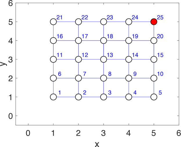
Figure 2: Graph ${\cal{G}}\!\setminus\!s$ of the non-source agent network used in simulations. The leader, shown in red, has access to the source $Z_{s}$.

The update gain $\gamma$ of the system in Eq. (13) without DSR is selected to ensure stability. The weight of each edge is selected as one, i.e., $a_{ij}=1$ in Eq. (6). The maximum value $\bar{\gamma}$ of the update gain $\gamma$ in Eq. (13) can be found from Lemma 1 as $\bar{\gamma}=0.2763$. The update gain $\gamma$ needs to be smaller than the maximum value to ensure stability without DSR, and therefore, the following simulations use the update gain

$$\gamma=0.1382=\frac{\bar{\gamma}}{2}<\bar{\gamma}.$$

The discrete time system without DSR in Eq. (13) settles to $2\%$ of the final value in $k_{Ts}=1331$ steps, and for a settling time of $T_{s}=1$ s, the sampling time is $\delta_{t}=T_{s}/k_{Ts}=7.5131\times 10^{-4}$.

IV-B Performance without and with DSR

The desired velocity of the source $Z_{s}$ is selected to increase, with a sinusoidal acceleration profile, from zero to the desired consensus value of

$$Z_{d}=0.02$$

as shown in Fig. 3. The response of the states $Z$ achieves the final desired value $Z_{d}$ with a settling time of $T_{s}=1$s to reach and stay within $2\%$ of the final value $Z_{d}$, as shown in Fig. 3.

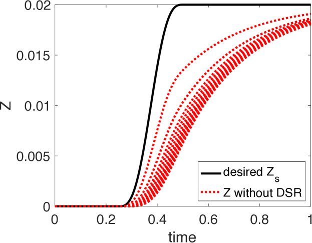
Figure 3: Response $Z$ of the standard consensus approach (without DSR) in Eq. (13), and the desired value $Z_{s}$ at the source.

The response with DSR is substantially faster when compared to the response without the DSR, for the same desired source $Z_{s}$. With the DSR gain selected as $\beta=0.95$ in Eq. (31), the settling time is $T_{s}=0.4756$s, i.e., to reach and stay within $2\%$ of the final value $Z_{d}$, as shown in Fig. 4. Thus, with a smaller settling time, the response with the DSR-based accelerated consensus is about $50\%$ faster than the response without DSR, as also seen by comparing the responses in Figs. 3 and 4.

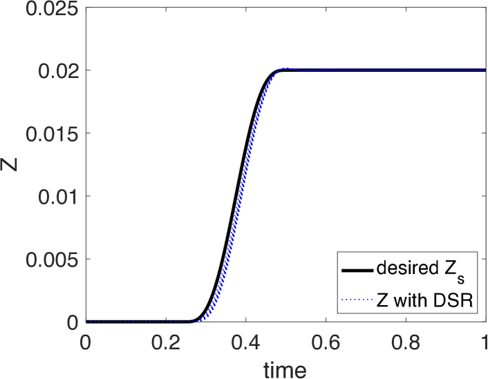
Figure 4: Response $Z$ of the accelerated-consensus approach implemented with DSR as in Eq. (31), for the same desired source time-profile $Z_{s}(t)$ as in Fig. 3

In addition to increasing the rate of convergence, and more importantly, the accelerated consensus leads to better synchronization during the transition. The deviation $\Delta$ (from synchronization) as in Eq. (32) of the response without the accelerated consensus as in Eq. (13) is $\Delta=0.0103$. The normalized deviation $\Delta^{*}$ in Eq. (34) is the same $\Delta^{*}=\Delta/T_{s}=0.0103$ since the settling time is $T_{s}=1$ without DSR. The use of the accelerated consensus reduces the loss of synchronization during the transition. The deviation $\Delta=0.0006$ for the accelerated consensus case. Even the normalized deviation (with a smaller settling time $T_{s}=0.4756$) for the accelerated consensus using DSR is $\Delta^{*}=0.0012$, which is about ten times smaller than the case without the DSR.

Thus, the proposed accelerated-consensus approach with DSR can substantially improve synchronization during the transition by about ten times, in addition to decreasing the transition time by about half, when compared to the case without the DSR approach.

IV-C Impact on formation spacing

To comparatively evaluate the impact of maintaining synchronization during the transition between consensus values, the state $Z$ of the agents are considered to represent the horizontal velocity $Z=V_{x}$ of each agent. Then, the horizontal position $X$ of each agent is found as

$$X[k+1] =X[k]+\delta_{t}V_{x}[k]~{}$$

$$=X[k]+\delta_{t}Z[k].$$ (35)

The initial and final positions with and without the accelerated consensus are compared in Fig. 5. As seen in the figure, the accelerated-consensus approach implemented with DSR as in Eq. (31) leads to better formation control when compared to the case without the DSR approach as in Eq. (13).

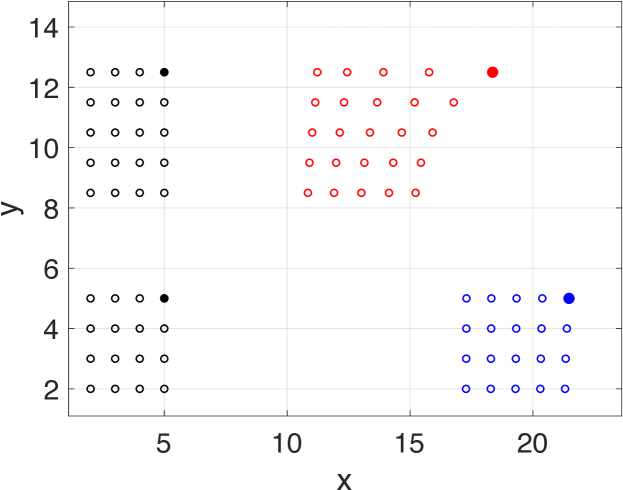
Figure 5: Accelerated consensus with DSR leads to better formation control when compared to the case without the DSR approach. Top (above $y=8$) shows the case without DSR with initial position in black and final position in red. Bottom (below $y=6$) shows the case with DSR-based accelerated consensus, with initial position in black and final position in blue.

In this example, no control actions are taken to maintain the formation to focus on the comparative evaluation of the performance with and without the proposed accelerated-consensus approach. Nevertheless, the ability of the accelerated-consensus approach to reduce distortions in the formation can potentially improve the performance of other methods with control actions to maintain the formation.

IV-D Summary of results

The use of the accelerated consensus, implemented using DSR, results in a faster convergence to the consensus value. Moreover, during the transition the network is more cohesive with the accelerated-consensus approach, which results in better formation control. While this article focussed on a quadratic potential with a linear network dynamics, the accelerated-consensus approach could also be implemented for the nonlinear case.

V Conclusions

This article showed that accelerated-gradient methods, used to improve the convergence in gradient-based search algorithms, can be used to improve current consensus algorithms in networked multi-agent systems. Moreover, the article developed implementation of the proposed accelerated consensus using delayed self reinforcement (DSR), where each agent only uses current and past information from the network. This is advantageous since the consensus improvement is achieved without the need to change the network connectivity and without the need for additional information from the network. Simulation results showed that the proposed accelerated-consensus approach with DSR can substantially improve synchronization during the transition by about ten times, in addition to decreasing the transition time by about half, when compared to the case without the DSR approach. This was shown to improve formation control during transitions in networked multi-agent systems.

References

- [1] A Huth and C Wissel. The simulation of the movement of fish schools. Journal of Theoretical Biology, 156(3):365–385, Jun 7 1992.
- [2] Tamás Vicsek, András Czirók, Eshel Ben-Jacob, Inon Cohen, and Ofer Shochet. Novel type of phase transition in a system of self-driven particles. Phys. Rev. Lett., 75:1226–1229, Aug 1995.
- [3] A. Jadbabaie, Jie Lin, and A. S. Morse. Coordination of groups of mobile autonomous agents using nearest neighbor rules. IEEE Transactions on Automatic Control, 48(6):988–1001, June 2003.
- [4] Wei Ren and R. W. Beard. Consensus seeking in multiagent systems under dynamically changing interaction topologies. IEEE Transactions on Automatic Control, 50(5):655–661, May 2005.
- [5] R. Olfati-Saber. Flocking for multi-agent dynamic systems: algorithms and theory. IEEE Transactions on Automatic Control, 51(3):401–420, March 2006.
- [6] Iasson Karafyllis and Markos Papageorgiou. Global Exponential Stability for Discrete-Time Networks With Applications to Traffic Networks. IEEE Transactions on Control of Network Systems, 2(1):68–77, Mar 2015.
- [7] J. M. Peng, J. N. Wang, and J. Y. Shan. Robust cooperative output tracking of networked high-order power integrators systems. International Journal of Control, 89(2):270–280, FEB 1 2016.
- [8] Deyuan Meng, Yingmin Jia, Kaiquan Cai, and Junping Du. Transcale average consensus of directed multi-vehicle networks with fixed and switching topologies. International Journal of Control, 90(10):2098–2110, 2017.
- [9] A. Attanasi, A. Cavagna, L Del Castello, I. Giardina, T.S. Grigera, A. Jelic, S. Melillo, L. Parisi, O. Pohl, E. Shen, and M. Viale. Information transfer and behavioural inertia in starling flocks. Nature Physics, 10(9):615–698, Sep 1 2014.
- [10] Hanlei Wang and Yongchun Xie. Flocking of networked mechanical systems on directed topologies: a new perspective. International Journal of Control, 88(4):872–884, APR 3 2015.
- [11] R. Olfati-Saber, J.A. Fax, and R.M. Murray. Consensus and cooperation in networked multi-agent systems. Proceedings of the IEEE, 95(1):215–233, Jan 2007.
- [12] S. Devasia. Faster Response Discrete-Time Networks under Update-Rate Limits. Fifth Indian Control Conference, IIT Delhi, India, pages 1–6, Jan, 9-11 2019.
- [13] Weisheng Chen, Shaoyong Hua, and Shuzhi Sam Ge. Consensus-based distributed cooperative learning control for a group of discrete-time nonlinear multi-agent systems using neural networks. Automatica, 50(9):2254–2268, Sep 2014.
- [14] Ruggero Carli, Fabio Fagnani, Alberto Speranzon, and Sandro Zampieri. Communication constraints in the average consensus problem. Automatica, 44(3):671–684, Mar 2008.
- [15] Maria Pia Fanti, Agostino Marcello Mangini, Francesca Mazzia, and Walter Ukovich. A new class of consensus protocols for agent networks with discrete time dynamics. Automatica, 54:1–7, Apr 2015.
- [16] D. E. Rumelhart, G. E. Hinton, and R. J. Williams. Learning Internal Representations by Error Propagation, pp. 318-362, in D. E. Rumelhart and J. L. McClelland (eds.) Parallel Distributed Processing, Vol. 1 . MIT Press, Cambridge, MA, 1986.
- [17] Ning Qian. On the momentum term in gradient descent learning algorithms. Neural Networks, 12(1):145 – 151, 1999.
- [18] Santosh Devasia. Rapid information transfer in networks with delayed self reinforcement. CoRR, http://arxiv.org/abs/1801.00910, 2018.
- [19] S. Devasia. Rapid Information Transfer in Swarms under Update-Rate-Bounds using Delayed Self Reinforcement. ASME 2018 Dynamic Systems and Control Conference (DSCC), Atlanta, GA, USA, pages 1–9, Sep. 30-Oct. 3 2018.
- [20] W. T. Tuttle. Graph Theory. Cambridge University Press, Cambridge, 2001.
- [21] R. Olfati-Saber and R. M. Murray. Consensus problems in networks of agents with switching topology and time-delays. IEEE Transactions on Automatic Control, 49(9):1520–1533, Sep. 2004.
- [22] Hui Zhang and Junmin Wang. Robust two-mode-dependent controller design for networked control systems with random delays modelled by Markov chains. International Journal of Control, 88(12):2499–2509, DEC 2 2015.