Two-Scale Methods for Convex Envelopes

Abstract.

We develop two-scale methods for computing the convex envelope of a continuous function over a convex domain in any dimension. This hinges on a fully nonlinear obstacle formulation [18]. We prove convergence and error estimates in the max norm. The proof utilizes a discrete comparison principle, a discrete barrier argument to deal with Dirichlet boundary values, and the property of flatness in one direction within the non-contact set. Our error analysis extends to a modified version of the finite difference wide stencil method of [19].

Key words. Convex envelope, fully-nonlinear obstacle, two-scale method, monotone, pointwise error estimates, Hölder regularity, flatness.

AMS subject classifications. 65N06, 65N12, 65N15, 65N30; 35J70, 35J87.

1. Introduction

Given an open set $\Omega\subset\mathbb{R}^{d}$ and a continuous function $f:\overline{\Omega}\rightarrow\mathbb{R}$, its convex envelop in $\Omega$ is defined as

(1.1) $$u(x)=\sup\left\{l(x):l\leq f\text{ in }\overline{\Omega},\;l\text{ is affine}\right\},$$

which in fact is the largest convex function majorized by $f$ in $\overline{\Omega}$. This function $u$ can also be viewed as the viscosity solution of the following fully nonlinear, degenerate elliptic PDE introduced by Oberman [18]

(1.2) $$T[u;f](x):=\min\left\{f(x)-u(x),\lambda_{1}[D^{2}u](x)\right\}=0,$$

where $\lambda_{1}[D^{2}u]$ denotes the smallest eigenvalue of the Hessian $D^{2}u$. This is the complementarity form of the fully nonlinear obstacle problem at hand.

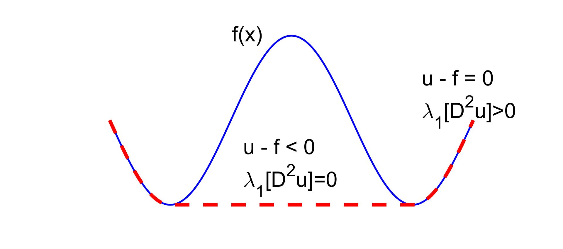
Figure 1. Illustration of the equation (1.2). In the non-contact set $\{u<f\}$, the function $u$ must be flat in one direction, i.e. $\lambda_{1}[D^{2}u]=0$.

Figure 1 illustrates the pde formulation (1.2). Roughly speaking, in the contact set

$$\mathcal{C}(f):=\left\{x\in\overline{\Omega}:u(x)=f(x)\right\},$$

we have the equality $u=f$ and the inequality $\lambda_{1}[D^{2}u]\geq 0$ given by the convexity of $u$. Outside the contact set, we have $u<f$ and that $u$ is flat in at least one direction which implies $\lambda_{1}[D^{2}u]=0$.

In this paper, we consider the case $\Omega$ bounded and strictly convex, which guarantees the Dirichlet boundary condition $u=f$ on $\partial\Omega$ is attained. Therefore the convex envelope $u$ of $f$ is the viscosity solution of the following problem:

(1.3) $$\left\{\begin{aligned} T[u;f](x)=\min\left\{f(x)-u(x),\lambda_{1}[D^{2}u](x)\right\}=0&\quad{\rm in}\;\;\Omega,\\ u=f&\quad{\rm on}\;\;\partial\Omega.\end{aligned}\right.$$

The regularity study of convex envelopes dates back to [25, 5], thus before the PDE formulation (1.3) of [18]. However, the problem considered in [25, 5] is a Dirichlet problem for the degenerate Monge-Ampère equation, $\det(D^{2}u)=0$, which corresponds to the convex envelope of function $f$ given on the boundary $\partial\Omega$ as a Dirichlet condition. For the convex envelope $u$ in (1.1), De Philippis and Figalli [6] obtained recently the optimal regularity $u\in C^{1,1}(\overline{\Omega})$ under the assumption that $\Omega$ is a uniformly convex domain of class $C^{3,1}$ and $f\in C^{3,1}(\overline{\Omega})$.

There are a handful of papers regarding the numerical approximation of convex envelopes. Oberman [19] proposed a wide stencil method to approximate (1.2). Dolzmann [7] developed a method to compute rank-one convex envelopes, a related notion of critical importance in materials science. Dolzmann and Walkington [8] proved an $O(h^{1/3})$ rate of convergence. Finally, Bartels [2] improved the error estimate of [8] to $O(h)$ upon increasing the number of directions and function evaluations within elements, thus at the expense of extra computational cost.

In this paper, we construct and study a two-scale method for (1.3), which is somewhat related to the wide stencil method of [19]. Two-scale methods are developed in [14], whereas suboptimal pointwise error estimates are derived in [15] and optimal ones in [13]. We prove existence, uniqueness, and uniform convergence, as well as pointwise error estimates under realistic regularity assumptions on $u$. Our proof hinges on a discrete comparison principle and discrete barrier functions, and is thus classical. However, we exploit that $u$ is flat in at least one direction outside the contact set $\mathcal{C}(f)$ [5, 21], a crucial property that plays an essential role in dealing with low regularity of $u$. Our techniques extend to a modified wide stencil method obtained from that in [19] upon adding a two-scale structure.

The remainder of this paper is organized as follows. In section 2, we introduce the two-scale method for convex envelope problem (1.3) and prove several properties of it. In section 3, we prove our main error estimate in the $L^{\infty}$ norm after reviewing geometric properties of $u$ and studying the consistency error. We next extend our analysis to a modified wide stencil method in section 4. We conclude in section 5 with numerical experiments which illustrate the performance of the two-scale methods and compare with theory.

2. Two-Scale Method

In this section, we extend the two-scale method developed in [14] to solve (1.3), and prove several important properties including convergence.

2.1. Definition of the Two-Scale Method

Let $\{\mathcal{T}_{h}\}$ be a sequence of meshes made of closed simplices $T$. Let $\mathcal{T}_{h}$ be shape-regular and quasi-uniform with mesh size $h$ and shape-regular constant $\sigma$, i.e.

(2.1) $$\max_{h}\ \max_{T\in\mathcal{T}_{h}}\ \frac{h_{T}}{\rho_{T}}\leq\sigma,$$

where $h_{T}$ denotes the diameter of $T$ and $\rho_{T}$ the diameter of the largest ball inscribed in $T$. Let $\Omega_{h}$ be the interior of the union of elements $T\in\mathcal{T}_{h}$, $\mathcal{N}_{h}$ be the nodes of $\mathcal{T}_{h}$, $\mathcal{N}_{h}^{b}:=\{x_{i}\in\mathcal{N}_{h}:x_{i}\in\partial\Omega\}$ be the boundary nodes and $\mathcal{N}_{h}^{0}:=\mathcal{N}_{h}\setminus\mathcal{N}_{h}^{b}$ be the interior nodes; since we require that $\mathcal{N}_{h}^{b}\subset\partial\Omega$ we deduce that $\Omega_{h}\subset\Omega$ is also convex. Let $\mathbb{V}_{h}$ be the space of continuous piecewise linear functions over $\mathcal{T}_{h}$.

Before introducing the two-scale method we need additional notation. Let $\mathbb{S}$ be the unit sphere in $\mathbb{R}^{d}$. We consider a finite discretization $\mathbb{S}_{\theta}\subset\mathbb{S}$ of $\mathbb{S}$ governed by the parameter $\theta$: given any $v\in\mathbb{S}$, there exists $v^{\theta}\in\mathbb{S}_{\theta}$ such that

$$|v-v^{\theta}|\leq\theta.$$

Let the meshsize $h$ be the fine scale and $\delta\geq h$ (to be chosen later) be the coarse scale. For every $x_{i}\in\mathcal{N}_{h}^{0}$, let

(2.2) $$\delta_{i}:=\min\big{\{}\delta,\textrm{dist}(x_{i},\partial\Omega_{h})\big{\}},$$

and observe that $\delta_{i}\geq C(\sigma)h$ and the open ball $B(x_{i},\delta_{i})$ centered at $x_{i}$ with radius $\delta_{i}$ is contained in $\Omega_{h}$. For any function $w\in C(\overline{\Omega}_{h})$, in particular for $w\in\mathbb{V}_{h}$, let the centered second difference operator be

(2.3) $$\nabla^{2}_{\delta}w(x_{i};v):=\frac{w(x_{i}+\delta_{i}v)-2w(x_{i})+w(x_{i}-\delta_{i}v)}{\delta_{i}^{2}}$$

and note that it is well defined for all $x_{i}\in\mathcal{N}_{h}^{0}$ and $v\in\mathbb{S}$. Since

(2.4) $$\lambda_{1}[D^{2}w](x)=\min_{v\in\mathbb{S}}\partial_{vv}^{2}w(x),$$

we consider the following approximation of $\lambda_{1}[D^{2}w]$ at $x=x_{i}\in\mathcal{N}_{h}^{0}$

$$\lambda_{1}[D^{2}w](x_{i})\approx\min_{v\in\mathbb{S}_{\theta}}\nabla^{2}_{\delta}w(x_{i};v).$$

If $\varepsilon:=(h,\delta,\theta)$ encodes the discretetization parameters, our two-scale operator $T_{\varepsilon}$ for the convex envelope problem (1.2) is finally given by

(2.5) $$T_{\varepsilon}[w_{h};f](x_{i})=\min\left\{f(x_{i})-w_{h}(x_{i}),\;\min_{v\in\mathbb{S}_{\theta}}\nabla^{2}_{\delta}w_{h}(x_{i};v)\right\}\quad\forall\,x_{i}\in\mathcal{N}_{h}^{0}$$

for any $w_{h}\in\mathbb{V}_{h}$. The corresponding two-scale method reads: seek $u_{\varepsilon}\in\mathbb{V}_{h}$

(2.6) $$T_{\varepsilon}[u_{\varepsilon};f](x_{i})=0\quad\;\forall x_{i}\in\mathcal{N}_{h}^{0},$$

and $u_{\varepsilon}(x_{i})=f(x_{i})$ for all $x_{i}\in\mathcal{N}_{h}^{b}$. We say that $w_{h}\in\mathbb{V}_{h}$ is a discrete subsolution (supersolution) of (2.6) if

$$T_{\varepsilon}[w_{h};f](x_{i})\geq 0\ (\leq 0)\quad\forall x_{i}\in\mathcal{N}_{h}^{0}\ ;\quad w_{h}(x_{i})\leq(\geq)f(x_{i})\quad\forall x_{i}\in\mathcal{N}_{h}^{b}.$$

Therefore, a discrete solution of (2.6) is both a discrete sub and supersolution.

Although this discrete solution $u_{\varepsilon}$ fails to be convex in general, it is still discretely convex, which is a notion of approximate convexity introduced in [14]. We say that $w_{h}\in\mathbb{V}_{h}$ is discretely convex [14] if

$$\nabla^{2}_{\delta}w_{h}(x_{i};v)\geq 0\qquad\forall x_{i}\in\mathcal{N}_{h}^{0},\quad\forall v\in\mathbb{S}_{\theta}.$$

2.2. Discrete Comparison Principle

One important feature of the definition (2.5) of the discrete operator $T_{\varepsilon}$ is its monotonicity. This is similar to the two-scale method for Monge-Ampère equation in [14, Lemma 2.3].

Lemma 2.1 (monotonicity).

Let $x_{i}\in\mathcal{N}_{h}^{0}$ be an interior node and $u_{h},w_{h}\in\mathbb{V}_{h}$. If $u_{h}(x_{i})\geq w_{h}(x_{i})$ and

$$\nabla^{2}_{\delta}u_{h}(x_{i};v)\leq\nabla^{2}_{\delta}w_{h}(x_{i};v)$$

for any $v\in\mathbb{S}_{\theta}$, then

$$T_{\varepsilon}[u_{h};f](x_{i})\leq T_{\varepsilon}[w_{h};f](x_{i}).$$

In particular, if $u_{h}-w_{h}$ attains a non-negative maximum at $x_{i}$, then

$$T_{\varepsilon}[u_{h};f](x_{i})\leq T_{\varepsilon}[w_{h};f](x_{i}).$$

Proof.

If $\nabla^{2}_{\delta}u_{h}(x_{i};v)\leq\nabla^{2}_{\delta}w_{h}(x_{i};v)$ for any $v\in\mathbb{S}_{\theta}$, then

$$\min_{v\in\mathbb{S}_{\theta}}\nabla^{2}_{\delta}u_{h}(x_{i};v)\leq\min_{v\in\mathbb{S}_{\theta}}\nabla^{2}_{\delta}w_{h}(x_{i};v).$$

Recalling the definition (2.5) of $T_{\varepsilon}$ and combining with the fact $u_{h}(x_{i})\geq w_{h}(x_{i})$, this implies

$$T_{\varepsilon}[u_{h};f](x_{i})\leq T_{\varepsilon}[w_{h};f](x_{i}).$$

On the other hand, if $u_{h}-w_{h}$ attains a non-negative maximum at $x_{i}\in\mathcal{N}_{h}^{0}$, then we have $u_{h}(x_{i})\geq w_{h}(x_{i})$ and

$$u_{h}(x_{i})-w_{h}(x_{i})\geq u_{h}(z)-w_{h}(z)\quad\forall z\in\overline{\Omega}_{h}.$$

By definition (2.3) of operator $\nabla^{2}_{\delta}$, we obtain

$$\nabla^{2}_{\delta}u_{h}(x_{i};v)\leq\nabla^{2}_{\delta}w_{h}(x_{i};v)\quad\forall v\in\mathbb{S}_{\theta},$$

and thus use the previous result to conclude the proof. ∎

Monotonicity leads to the following discrete comparison principle.

Lemma 2.2 (discrete comparison principle).

Let $u_{h},w_{h}\in\mathbb{V}_{h}$ with $u_{h}(x_{i})\leq w_{h}(x_{i})$ for all $x_{i}\in\mathcal{N}_{h}^{b}$ and

(2.7) $$T_{\varepsilon}[u_{h};f](x_{i})\geq T_{\varepsilon}[w_{h};f](x_{i})\quad\forall x_{i}\in\mathcal{N}_{h}^{0}.$$

Then, $u_{h}\leq w_{h}$ in $\Omega_{h}$.

Proof.

The proof splits into two steps.

Step 1. We first consider the case with strict inequality

(2.8) $$T_{\varepsilon}[u_{h};f](x_{i})>T_{\varepsilon}[w_{h};f](x_{i})\quad\forall x_{i}\in\mathcal{N}_{h}^{0}.$$

We assume by contradiction that there exists an interior node $x_{k}\in\mathcal{N}_{h}^{0}$ such that $u_{h}-w_{h}$ attains a maximum at $x_{k}$, and $u_{h}(x_{k})>w_{h}(x_{k})$. Then, by 2.1 (monotonicity) we obtain the contradiction

(2.9) $$T_{\varepsilon}[u_{h};f](x_{k})\leq T_{\varepsilon}[w_{h};f](x_{k}).$$

Step 2. Now we deal with (2.7) without the strict inequality. We introduce the auxiliary strictly convex function $q(x)=\frac{1}{2}|x-x_{0}|^{2}-\frac{1}{2}R^{2}$, which satisfies $q\leq 0$ on $\overline{\Omega}$, and in particular $q\leq 0$ on $\partial\Omega_{h}$ provided $R=\textrm{diam}(\Omega)$ and $x_{0}\in\Omega$. Its Lagrange interpolant $q_{h}=\mathcal{I}_{h}q$ is discretely convex and satisfies

$$\nabla^{2}_{\delta}q_{h}(x_{i};v)\geq\nabla^{2}_{\delta}q(x_{i};v)=\partial^{2}_{vv}q(x_{i})=1\quad\forall x_{i}\in\mathcal{N}_{h}^{0},\quad\forall v\in\mathbb{S}_{\theta},$$

because $q$ is quadratic. For arbitrary $\alpha>0$, consider the function $u_{\alpha}=u_{h}+\alpha q_{h}-\alpha$, which satisfies $u_{\alpha}<u_{h}\leq w_{h}$ on $\partial\Omega_{h}$ and

$$T_{\varepsilon}[u_{\alpha};f](x_{i}) =\min\left\{f(x_{i})-u_{\alpha}(x_{i}),\;\min_{v\in\mathbb{S}_{\theta}}\nabla^{2}_{\delta}u_{\alpha}(x_{i})(x_{i};v)\right\}$$

$$\geq\min\left\{f(x_{i})-(u_{h}(x_{i})-\alpha),\;\min_{v\in\mathbb{S}_{\theta}}\left(\nabla^{2}_{\delta}u_{h}(x_{i};v)+\alpha\right)\right\}$$

$$=T_{\varepsilon}[u_{h};f](x_{i})+\alpha>T_{\varepsilon}[w_{h};f](x_{i})\quad\forall x_{i}\in\mathcal{N}_{h}^{0}.$$

Applying Step 1 we deduce

$$u_{h}+\alpha q_{h}-\alpha\leq w_{h}\quad\forall\alpha>0.$$

Finally, let $\alpha\to 0$ to obtain the asserted inequality. ∎

2.3. Existence, Uniqueness and Stability

We now prove several properties of our discrete system (2.6) which are useful for the proof of convergence.

Lemma 2.3 (existence, uniqueness and stability).

There exists a unique $u_{\varepsilon}\in\mathbb{V}_{h}$ that solves the discrete equation (2.6). The solution $u_{\varepsilon}$ is stable in the sense that $\|u_{\varepsilon}\|_{L^{\infty}(\Omega_{h})}\leq\|f\|_{L^{\infty}(\Omega)}$ regardless of the parameters $\varepsilon=(h,\delta,\theta)$ of the method.

Proof.

Since uniqueness is a trivial consequence of Lemma 2.2 (discrete comparison principle), we just have to prove existence and stability.

Step 1 - Stability: We first show that $u_{h}^{-}=\mathcal{I}_{h}u$ is a discrete subsolution where $u$ is the exact convex envelope and $u_{h}^{+}=\mathcal{I}_{h}f$ is a discrete supersolution, where again $\mathcal{I}_{h}$ stands for the Lagrange interpolation operator.

Since $u$ is the exact convex envelope, for any $x_{i}\in\mathcal{N}_{h}^{0}$, we have $u_{h}^{-}(x_{i})\leq f(x_{i})$ and $\nabla^{2}_{\delta}u_{h}^{-}(x_{i};v)\geq 0$ because $u$ is convex. By definition (2.5) of $T_{\varepsilon}$, this gives us $T_{\varepsilon}[u_{h}^{-};f](x_{i})\geq 0$ for all $x_{i}\in\mathcal{N}_{h}^{0}$. It is also clear that we have $T_{\varepsilon}[u_{h}^{+};f](x_{i})\leq f(x_{i})-u_{h}^{+}(x_{i})=0$ for all $x_{i}\in\mathcal{N}_{h}^{0}$. Therefore combining with the fact that $u_{h}^{+}(x_{i})=u_{h}^{-}(x_{i})=f(x_{i})$ for $x_{i}\in\mathcal{N}_{h}^{b}$, we see that $u_{h}^{-}$ and $u_{h}^{+}$ are discrete subsolution and supersolution respectively. By Lemma 2.2 (discrete comparison principle), this implies

(2.10) $$u_{h}^{-}\leq u_{\varepsilon}\leq u_{h}^{+},$$

and we thus obtain the stability of $u_{\varepsilon}$ because both $\|u_{h}^{-}\|_{L^{\infty}(\Omega_{h})}$ and $\|u_{h}^{+}\|_{L^{\infty}(\Omega_{h})}$ are bounded by $\|f\|_{L^{\infty}(\Omega)}$.

Step 2 - Discrete Perron Method: It remains to prove the existence of $u_{\varepsilon}$. We proceed as in [14, 17] and use the discrete Perron’s method to construct a monotone increasing sequence of functions $\left\{u_{h}^{k}\right\}_{k=0}^{\infty}$. The initial iterate $u_{h}^{0}$ is chosen to be $u_{h}^{-}$, and thus satisfies the boundary condition $u_{h}^{0}(x_{i})=f(x_{i})$ for all $x_{i}\in\mathcal{N}_{h}^{b}$ and

(2.11) $$T_{\varepsilon}[u_{h}^{0};f](x_{i})\geq 0\quad\forall x_{i}\in\mathcal{N}_{h}^{0}.$$

We construct $\left\{u_{h}^{k}\right\}$ by induction. Suppose that we have already built $u_{h}^{k}\in\mathbb{V}_{h}$ satisfying both the boundary condition and (2.11). To construct $u_{h}^{k+1}\in\mathbb{V}_{h}$ such that $u_{h}^{k+1}\geq u_{h}^{k}$ and also satisfies both the boundary condition and (2.11), we consider all interior nodes in order and construct auxiliary functions $u_{h}^{k,i-1}\in\mathbb{V}_{h}$ using the first $i-1$ nodes and starting from $u_{h}^{k,0}:=u_{h}^{k}$ as follows. At $x_{i}\in\mathcal{N}_{h}^{0}$ we check whether or not $T_{\varepsilon}[u_{h}^{k,i-1};f](x_{i})>0$. If so, we increase the value of $u_{h}^{k,i-1}(x_{i})$ and denote the resulting function by $u_{h}^{k,i}$, until

$$T_{\varepsilon}[u_{h}^{k,i};f](x_{i})=0.$$

This is possible because $T_{\varepsilon}[u_{h}^{k,i};f](x_{i})$ is strictly decreasing with respect to $u_{h}^{k,i}(x_{i})$. Expression (2.5) also shows that this process does not decrease $T_{\varepsilon}[u_{h}^{k,i};f](x_{j})$ for any $x_{j}\neq x_{i}$, whence

$$T_{\varepsilon}[u_{h}^{k,i};f](x_{j})\geq T_{\varepsilon}[u_{h}^{k,i-1};f](x_{j})\geq 0\quad\forall x_{j}\neq x_{i}.$$

We repeat this process with the remaining nodes $x_{j}$ for $i<j\leq N$ where $N$ is the number of all interior points, and set $u_{h}^{k+1}:=u_{h}^{k,N}$ to be the last intermediate function. By construction, we clearly obtain

$$T_{\varepsilon}[u_{h}^{k+1};f](x_{i})\geq 0,\quad u_{h}^{k+1}(x_{i})\geq u_{h}^{k}(x_{i})\quad\forall x_{i}\in\mathcal{N}_{h}^{0},$$

and $u_{h}^{k}(x_{i})=f(x_{i})$ for all $x_{i}\in\mathcal{N}_{h}^{b}$.

Step 3 - Convergence of $u_{h}^{k}$: By construction we have $u_{h}^{k}\geq u_{h}^{0}=u_{h}^{-}$ and by 2.2 (discrete comparison principle), $u_{h}^{k}\leq u_{h}^{+}$ and thus $u_{h}^{k}(x_{i})$ is uniformly bounded. Since the sequence $\{u_{h}^{k}\}_{k}$ is monotone, it must converge to a limit

$$u_{\varepsilon}(x_{i})=\lim_{k\to\infty}u_{h}^{k}(x_{i})=\lim_{k\to\infty}u_{h}^{k,i}(x_{i})\quad\forall x_{i}\in\mathcal{N}_{h}.$$

Due to continuity of $T_{\varepsilon}[w_{h};f]$ with respect to $w_{h}(x_{j})$, we have $T_{\varepsilon}[u_{\varepsilon};f](x_{i})=\lim_{k\to\infty}T_{\varepsilon}[u_{h}^{k,i};f](x_{i})=0$ for any $x_{i}\in\mathcal{N}_{h}^{0}$. This implies that the limit $u_{\varepsilon}$ is the solution of discrete equation (2.6) and finishes the proof. ∎

Another way to prove existence and uniqueness is to take advantage of the existing results for Bellman equation and Howard’s algorithm as we can see in section 5.

We define for $x\in\overline{\Omega}$

(2.12) $$\overline{u}(x):=\limsup_{\varepsilon,\frac{h}{\delta}\to 0,\;y\to x}u_{\varepsilon}(y),\quad\underline{u}(x):=\liminf_{\varepsilon,\frac{h}{\delta}\to 0,\;y\to x}u_{\varepsilon}(y),$$

where the limits are taken for $y\in\Omega_{h}$. From equation (2.10) and the continuity of both $u$ and $f$, we immediately obtain the following lemma characterizing the behavior of $\overline{u}$ and $\underline{u}$ on the boundary $\partial\Omega$.

Lemma 2.4 (boundary behavior).

Let $\Omega$ be a strictly convex bounded domain, let $u_{\varepsilon}$ be the discrete solution of (2.6), and let $\overline{u}(x)$ and $\underline{u}(x)$ be defined in (2.12). Then we have $\overline{u}(x)=\underline{u}(x)=f(x)$ for all $x\in\partial\Omega$.

Proof.

Since $\Omega$ is strictly convex, the Dirichlet boundary condition $u=f$ on $\partial\Omega$ is attained as a direct consequence of [23, Corollary 17.1.5], or can be proved in the same way as [10, Theorem 1.5.2]. Next use

$$\mathcal{I}_{h}u(x)=u_{h}^{-}(x)\leq u_{\varepsilon}(x)\leq u_{h}^{+}(x)=\mathcal{I}_{h}f(x)\quad x\in\Omega_{h}$$

with equality on $\partial\Omega$ to deduce the assertion. ∎

2.4. Consistency

We now quantify the consistency error of our discrete operator $T_{\varepsilon}[\mathcal{I}_{h}u;f]$ for a smooth function $u$, which is enough for the proof of convergence. In Section 3 we will carry out a more delicate analysis of the consistency error which enables us to prove error estimates for solutions with weaker but realistic regularity. In the meantime, we stress that the convex envelope $u$ is generically never better than of class $C^{1,1}(\overline{\Omega})$ [6].

Given a node $x_{i}\in\mathcal{N}_{h}^{0}$ we denote

(2.13) $$B_{i}:=\cup\{T:T\in\mathcal{T}_{h},\,\textrm{dist}(x_{i},T)\leq\delta_{i}\},$$

where $\delta_{i}$ is defined in (2.2). We also denote by $\Omega_{h,s}$ the following $s$-interior region of $\Omega_{h}$ for any parameter $s>0$

$$\Omega_{h,s}=\left\{x\in\Omega_{h}\;:\;\textrm{dist}(x,\partial\Omega_{h})\geq s\right\}.$$

Hereafter, we use the symbols $C(d,\sigma)$, $C(d)$ and $C$ to denote constants that depend only on the dimension $d$ and the shape-regularity constant $\sigma$, but are independent of the two scales $h$ and $\delta$, the parameter $\theta$ and the function $u$.

2.5 below establishes a consistency error estimate for the two-scale method similar to [14, Lemma 4.1] and [14, Lemma 4.2]. The proof follows along the lines of [14].

Lemma 2.5 (consistency for smooth functions).

Let $u\in C^{2+k,\alpha}(B_{i})$ for $k=0,1$ and $\alpha\in(0,1]$, $\mathcal{I}_{h}u$ be its Lagrange interpolant, and $B_{i}$ be defined in (2.13). The following estimates are then valid:

1. For all $x_{i}\in\mathcal{N}_{h}^{0}$ and all $v\in\mathbb{S}$, we have

   (2.14) $$\left|\nabla^{2}_{\delta}\mathcal{I}_{h}u(x_{i};v)\right|\leq C(d,\sigma)\;|u|_{W^{2}_{\infty}(B_{i})},$$

2. For all $x_{i}\in\mathcal{N}_{h}^{0}\cap\Omega_{h,\delta}$ and all $v\in\mathbb{S}$, we have

   (2.15) $$\left|\nabla^{2}_{\delta}\mathcal{I}_{h}u(x_{i};v)-\frac{\partial^{2}u}{\partial{v}^{2}}(x_{i})\right|\leq C(d,\sigma)\left(|u|_{C^{2+k,\alpha}(B_{i})}\delta^{k+\alpha}+|u|_{W^{2}_{\infty}(B_{i})}\frac{h^{2}}{\delta^{2}}\right),$$

3. For all $x_{i}\in\mathcal{N}_{h}^{0}\cap\Omega_{h,\delta}$ and all $v\in\mathbb{S}$, we have

   (2.16) $$\small\bigg{|}T_{\varepsilon}[\mathcal{I}_{h}u;f](x_{i})-T[u;f](x_{i})\bigg{|}\leq C(d,\sigma)\left[|u|_{C^{2+k,\alpha}(B_{i})}\delta^{k+\alpha}+|u|_{W^{2}_{\infty}(B_{i})}\left(\frac{h^{2}}{\delta^{2}}+\theta^{2}\right)\right].$$

Proof.

For the proof of (2.14) and (2.15), the readers may refer to [14, Lemma 4.1]. Here we only prove (2.16).

Recalling the definitions of $T$ in (1.2) and $T_{\varepsilon}$ in (2.5) we only need to prove

$$\left|\lambda_{1}[D^{2}u](x_{i})-\min_{v\in\mathbb{S}_{\theta}}\nabla^{2}_{\delta}\mathcal{I}_{h}u(x_{i};v)\right|\leq C(d,\sigma)\left[|u|_{C^{2+k,\alpha}(B_{i})}\delta^{k+\alpha}+|u|_{W^{2}_{\infty}(B_{i})}\left(\frac{h^{2}}{\delta^{2}}+\theta^{2}\right)\right].$$

To this end, first let $v_{\theta}$ be the direction such that

$$\nabla^{2}_{\delta}\mathcal{I}_{h}u(x_{i};v_{\theta})=\min_{v\in\mathbb{S}_{\theta}}\nabla^{2}_{\delta}\mathcal{I}_{h}u(x_{i};v).$$

We use (2.4) and (2.15) to get

$$\lambda_{1}[D^{2}u](x_{i})-\min_{v\in\mathbb{S}_{\theta}}\nabla^{2}_{\delta}\mathcal{I}_{h}u(x_{i};v)\leq \;\frac{\partial^{2}u}{\partial{v_{\theta}}^{2}}(x_{i})-\nabla^{2}_{\delta}\mathcal{I}_{h}u(x_{i};v_{\theta})$$

$$\leq \;C(d,\sigma)\left(|u|_{C^{2+k,\alpha}(B_{i})}\delta^{k+\alpha}+|u|_{W^{2}_{\infty}(B_{i})}\frac{h^{2}}{\delta^{2}}\right),$$

which proves one inequality of (2.16). To show the reverse inequality we let $v$ be the direction that realizes the minimum in (2.4), which means

$$\partial_{vv}^{2}u(x_{i})=\lambda_{1}[D^{2}u](x_{i}),$$

and we also know that $v$ is the eigenvector of $D^{2}u(x_{i})$ corresponding to the smallest eigenvalue $\lambda_{1}$. By definition of $\mathbb{S}_{\theta}$, there exists $v_{\theta}\in\mathbb{S}_{\theta}$ such that $|v-v_{\theta}|\leq\theta$, and we can thus write

$$\min_{v\in\mathbb{S}_{\theta}}\nabla^{2}_{\delta}\mathcal{I}_{h}u(x_{i};v)-\lambda_{1}[D^{2}u](x_{i})\leq\nabla^{2}_{\delta}\mathcal{I}_{h}u(x_{i};v_{\theta})-\partial_{vv}^{2}u(x_{i})=I_{1}+I_{2},$$

where

$$I_{1}=\nabla^{2}_{\delta}\mathcal{I}_{h}u(x_{i};v_{\theta})-\partial_{v_{\theta}v_{\theta}}^{2}u(x_{i}),\qquad I_{2}=\partial_{v_{\theta}v_{\theta}}^{2}u(x_{i})-\partial_{vv}^{2}u(x_{i}).$$

It is clear that $I_{1}$ can be bounded by (2.15). For $I_{2}$, write $v_{\theta}=v+w$, then

$$\partial_{v_{\theta}v_{\theta}}^{2}u(x_{i}) =v_{\theta}^{T}D^{2}u(x_{i})v_{\theta}=\partial_{vv}^{2}u(x_{i})+2w^{T}D^{2}u(x_{i})v+w^{T}D^{2}u(x_{i})w$$

$$=\partial_{vv}^{2}u(x_{i})+2\lambda_{1}v\cdot w+w^{T}D^{2}u(x_{i})w.$$

Since

$$1=|v_{\theta}|^{2}=|v|^{2}+2v\cdot w+|w|^{2},$$

and $|v|=1$, we observe that

$$|v\cdot w|=\frac{1}{2}|w|^{2}\leq\frac{1}{2}\theta^{2},$$

whence we obtain

$$I_{2}\leq C|u|_{W^{2}_{\infty}(B_{i})}\theta^{2}.$$

Combining the bounds for both $I_{1}$ and $I_{2}$ we have

$$\min_{v\in\mathbb{S}_{\theta}}\nabla^{2}_{\delta}\mathcal{I}_{h}u(x_{i};v)-\lambda_{1}[D^{2}u](x_{i})\leq C(d,\sigma)\left[|u|_{C^{2+k,\alpha}(B_{i})}\delta^{k+\alpha}+|u|_{W^{2}_{\infty}(B_{i})}\left(\frac{h^{2}}{\delta^{2}}+\theta^{2}\right)\right].$$

This finishes the proof of (2.16). ∎

2.5. Convergence

We are now ready to prove the convergence result.

Theorem 2.6 (convergence).

If $\Omega$ is a bounded and strictly convex domain and $f\in C(\overline{\Omega})$, then the discrete solution $u_{\varepsilon}$ of (2.6) converges uniformly to the convex envelope $u$ of $f$ as $\varepsilon=(h,\delta,\theta)\to 0$ and $\frac{h}{\delta}\to 0$.

Proof.

Our approximation scheme (2.6) satisfies monotonicity (2.2), stability (2.3), and consistency (2.5). Moreover, the PDE (1.3) for the convex envelope problem admits a comparison principle [20, Proposition 2.7] for Dirichlet boundary conditions in the classical sense. Similarly to [12, Section 4], [9, Theorem 17] and [14, Section 5], in order to use the convergence theorem of Barles and Souganidis [1], we still need the additional fact that $\overline{u}(x)=\underline{u}(x)=f(x)$ on $\partial\Omega$. Since this is proved in 2.4 (boundary behavior), [1] yields uniform convergence of the discrete solution $u_{\varepsilon}$ to the viscosity solution $u$ of (1.3). ∎

3. Rates of Convergence

In this section, we prove convergence rates for solutions of class $C^{k,\alpha}(\overline{\Omega})$ for $k=0,1$ and $0<\alpha\leq 1$. Since in general we could only expect $u\in C^{1,1}(\overline{\Omega})$ even for smooth $f$ and $\Omega$, our estimate of consistency error in Section 2.4 fails. The challenge is thus to estimate the consistency error for solutions with less regularity. We first show a key geometric lemma about convex envelopes which enables us to give an estimate of the consistency error for $u\in C^{k,\alpha}(\overline{\Omega})$. On the basis on this result, we next prove the convergence rate using 2.2 (discrete comparison principle).

3.1. Flatness

The heuristic behind the governing PDE (1.2) is that the convex envelope $u$ must be flat at least in one direction within the non-contact set, i.e. $\lambda_{1}[D^{2}u](x)=0$ for all $x\notin\mathcal{C}(f)$. The question whether there is a line segment containing $x$, on which $u$ is flat, is studied in [21, Section 3] for the Dirichlet convex envelope problem in which $f$ is only defined on $\partial\Omega$. For $f\in C(\overline{\Omega})$ defined in the entire $\Omega$, and corresponding definition (1.1) of convex envelope $u$, we have a similar property.

Lemma 3.1 (flatness in one direction).

Let $f\in C(\overline{\Omega})$ and $x\in\Omega$ be such that $\textrm{dist}(x,\mathcal{C}(f))\geq d\delta$. Then for any slope $p\in\partial u(x)$, there exists a direction $v\in\mathbb{S}$ such that

$$x_{\pm}=x\pm\delta v,\quad u(x_{\pm})=u(x)\pm\delta(p\cdot v),\quad\nabla^{2}_{\delta}u(x;v)=0.$$

Moreover, $p$ belongs also to the subdifferential sets $\partial u(x_{\pm})$.

This lemma says that if $x$ is away from the contact set $\mathcal{C}(f)$ at least at distance $d\delta$, then there exists a line segment centered at $x_{i}$ with length at least $2\delta$ such that the convex envelope $u$ is flat on this segment. The flattness means the second difference of $u$ in this direction is $0$, which plays an important role in obtaining consistency error for $x$ far away from $\mathcal{C}(f)$. To prove 3.1, we need the following definition and subsequent result: given $x\in\Omega\setminus\mathcal{C}(f)$ and $p\in\partial u(x)$, let

$$\mathcal{C}(f;x,p):=\left\{y\in\overline{\Omega}:f(y)=u(x)+p\cdot(y-x)\right\},$$

and note that $\mathcal{C}(f;x,p)\subset\mathcal{C}(f)$ because $u$ is convex and $u(y)\geq u(x)+p\cdot(y-x)$ whence $u(y)=f(y)$. The following auxiliary result is exactly the same as [6, Lemma 3.3] and similar to [5, Lemma 2] and [21, Theorem 3.2]. We still give a proof here for completeness.

Lemma 3.2 (structure of non-contact set).

Let $f\in C(\overline{\Omega})$ and $x\in\Omega\setminus\mathcal{C}(f)$. Then for any slope $p\in\partial u(x)$, there exist points $x_{1},\ldots,x_{k}\in\mathcal{C}(f)$ with $2\leq k\leq d+1$ such that

$$x\in\textrm{conv}\;(x_{1},\ldots,x_{k}),$$

and $u$ is affine in the convex hull $\textrm{conv}\;(x_{1},\ldots,x_{k})$ of $(x_{i})_{i=1}^{k}$. Moreover, $p$ is also in the subdifferential set $\partial u(y)$ for any $y\in\textrm{conv}\;(x_{1},\ldots,x_{k})$.

Proof.

For any $p\in\partial u(x)$, define $P(y):=u(x)+p\cdot(y-x)$ and observe that

$$\mathcal{C}:=\mathcal{C}(f;x,p)=\left\{y\in\overline{\Omega}:f(y)=P(y)\right\}.$$

We claim that $x\in\textrm{conv}(\mathcal{C})$. Argue by contradiction, suppose $x\notin\textrm{conv}(\mathcal{C})$, and use the hyperplane separation theorem to find an affine function $L$ such that $L(x)>0$ and $L(y)<0$ for every $y\in\mathcal{C}$. By the definition of $\mathcal{C}$ and the fact that $P\leq u\leq f$, it is clear that $f-P$ is strictly positive in the compact set $\overline{\Omega}\cap\{L\geq 0\}$: in fact, if $f(y)\leq P(y)$ then $f(y)=P(y)=u(y)$ and $y\in\mathcal{C}$, whence $L[y]<0$. Therefore it is easy to see that for some small $\alpha>0$, we have

$$\widetilde{L}(y):=P(y)+\alpha L(y)\leq f(y)\quad\forall y\in\overline{\Omega},$$

but $\widetilde{L}(x)>P(x)=u(x)$. This contradicts the definition of convex envelope $u$ and thus proves the claim $x\in\textrm{conv}(\mathcal{C})$. Now we use Carathéodory’s theorem to obtain the existence of $x_{1},\ldots,x_{k}\in\mathcal{C}$ with $k\leq d+1$ such that $x\in\textrm{conv}(x_{1},\ldots,x_{k})$.

To prove that $p\in\partial u(y)$ for any $y\in\textrm{conv}(x_{1},\ldots,x_{k})$, we define

$$\mathcal{K}:=\left\{y\in\overline{\Omega}:u(y)=u(x)+p\cdot(y-x)\right\}=\left\{y\in\overline{\Omega}:u(y)=P(y)\right\},$$

whence $u$ is affine in $\mathcal{K}$. We claim that $\mathcal{K}$ is convex. Let $y_{1},y_{2}\in\mathcal{K},\lambda\in(0,1)$ and $z=\lambda y_{1}+(1-\lambda)y_{2}$. Since $u$ is convex, we have

$$u(z)\leq\lambda u(y_{1})+(1-\lambda)u(y_{2})=\lambda P(y_{1})+(1-\lambda)P(y_{2})=P(z).$$

On the other hand, since $p\in\partial u(x)$, the supporting plane $P$ must be below $u$, and in particular

$$u(z)\geq P(z).$$

Therefore $u(z)=P(z)$, and thus $z\in\mathcal{K}$, which implies the convexity of $\mathcal{K}$. Since $P\leq u\leq f$, we have $\{x_{1},\ldots,x_{k}\}\subset\mathcal{C}\subset\mathcal{K}$ and $\textrm{conv}\;(x_{1},\ldots,x_{k})\subset\mathcal{K}$. It is clear that for any $y\in\mathcal{K}$, we have $u(y)=u(x)+p\cdot(y-x)$ and

$$P(z)=u(x)+p\cdot(z-x)=u(y)+p\cdot(z-y)\leq u(z)\quad\forall z\in\overline{\Omega}.$$

By definition of $\partial u(y)$ this implies $p\in\partial u(y)$ for any $y\in\textrm{conv}(x_{1},\ldots,x_{k})$. In addition, $u$ is affine in $\textrm{conv}\;(x_{1},\ldots,x_{k})$. ∎

Proof of 3.1.

For any $p\in\partial u(x)$, by 3.2 (structure of non-contact set), there exist $k$ ($2\leq k\leq d+1$) points $x_{i}\in\mathcal{C}(f;x,p)$ such that

$$x=\sum_{i=1}^{k}\lambda_{i}x_{i},\quad\lambda_{i}\geq 0,\quad\sum_{i=1}^{k}\lambda_{i}=1,$$

and $p$ belongs to the subdifferential set $\partial u(y)$ for any $y\in\textrm{conv}(x_{1},\ldots,x_{k})$. If $j$ is such that $\lambda_{j}=\max_{1\leq i\leq k}\lambda_{i}$, then we have

$$\lambda_{j}\geq\frac{1}{k}\sum_{i=1}^{k}\lambda_{i}=\frac{1}{k}\geq\frac{1}{d+1}.$$

Now let $x_{0}=\sum_{i\neq j}\frac{\lambda_{i}}{1-\lambda_{j}}x_{i}\in\textrm{conv}\;(x_{1},\ldots,x_{k})$ to get

$$x=\sum_{i=1}^{k}\lambda_{i}x_{i}=\lambda_{j}x_{j}+\sum_{i\neq j}\lambda_{i}x_{i}=\lambda_{j}x_{j}+(1-\lambda_{j})x_{0}.$$

Since both $x_{0},x_{j}\in\textrm{conv}\;(x_{1},\ldots,x_{k})$, the segment $\overline{x_{0}x_{j}}$ is also in $\textrm{conv}\;(x_{1},\ldots,x_{k})$. Due to the fact $\textrm{dist}(x,\mathcal{C}(f))\geq d\delta$, we have $|x_{j}-x|\geq d\delta$, and

$$|x_{0}-x|=\frac{\lambda_{j}}{1-\lambda_{j}}|x_{j}-x|\geq\frac{1/(d+1)}{1-1/(d+1)}\;d\delta=\delta.$$

Therefore, if $v=\frac{x_{j}-x}{|x_{j}-x|}$ and $x_{\pm}=x\pm\delta v$, clearly $x_{\pm}$ lie in the segment $\overline{x_{0}x_{j}}$, and thus also inside $\textrm{conv}(x_{1},\ldots,x_{k})$. Finally, 3.2 (structure of non-contact set) shows $p\in\partial u(x_{\pm})$ and $u(x_{\pm})=u(x)\pm\delta(p\cdot v)$, which immediately leads to $\nabla^{2}_{\delta}u(x;v)=0$. ∎

3.2. Consistency for Solutions with Hölder Regularity

In this section, we take advantage of results in Section 3.1 to derive a consistency error for solutions with realistic Hölder regularity $u\in C^{k,\alpha}(\overline{\Omega})$ for $k=0,1$ and $0<\alpha\leq 1$, which improves upon the consistency error estimates in Section 2.4.

The Lagrange interpolant $\mathcal{I}_{h}u\in\mathbb{V}_{h}$ of $u$ satisfies for all interior nodes $x_{i}\in\mathcal{N}_{h}^{0}$

$$\mathcal{I}_{h}u(x_{i})=u(x_{i})\leq f(x_{i}),\quad\nabla^{2}_{\delta}\mathcal{I}_{h}u(x_{i};v)\geq\nabla^{2}_{\delta}u(x_{i};v)\geq 0\quad\forall v\in\mathbb{S}$$

because of the convexity of $u$. In view of definition (2.5) of $T_{\varepsilon}$, this in turn implies $T_{\varepsilon}[\mathcal{I}_{h}u;f](x_{i})\geq 0$ for all $x_{i}\in\mathcal{N}_{h}^{0}$. The following proposition yields upper bounds for $T_{\varepsilon}[\mathcal{I}_{h}u;f](x_{i})$ depending on the location of $x_{i}$ relative to $\mathcal{C}(f)$ and $\partial\Omega$.

Proposition 3.3 (consistency for $u$ with Hölder regularity).

Let $\Omega$ be a bounded strictly convex domain, $u\in C^{k,\alpha}(\overline{\Omega})$ for $k=0,1$ and $0<\alpha\leq 1$ be the exact solution of the convex envelope problem (1.3). In addition, let $B_{i}$ be defined in (2.13) and set

(3.1) $$\widetilde{B_{i}}:=\{x\in\overline{\Omega}:|x-x_{i}|\leq d\delta\}.$$

For $x_{i}\in\mathcal{N}_{h}^{0}$, the following estimates are then valid:

1. If $\textrm{dist}(x_{i},\mathcal{C}(f))\geq d\delta$, we have

   (3.2) $$\min_{v_{\theta}\in\mathbb{S}_{\theta}}\nabla^{2}_{\delta}\mathcal{I}_{h}u(x_{i};v_{\theta})\leq C(d,\sigma)\frac{(\delta\theta)^{k+\alpha}+h^{k+\alpha}}{\delta^{2}}|u|_{C^{k,\alpha}(B_{i})}.$$

2. If $\textrm{dist}(x_{i},\mathcal{C}(f))<d\delta,\;\textrm{dist}(x_{i},\partial\Omega)\geq d\delta$, and $f\in C^{k,\alpha}(\overline{\Omega})$, then for $k=0$ we have

   (3.3) $$f(x_{i})-u(x_{i})\leq C(d,\sigma)\delta^{\alpha}\left(|u|_{C^{0,\alpha}(\widetilde{B_{i}})}+|f|_{C^{0,\alpha}(\widetilde{B_{i}})}\right),$$

   whereas for $k=1$ we have

   (3.4) $$f(x_{i})-u(x_{i})\leq C(d,\sigma)\delta^{1+\alpha}|f|_{C^{1,\alpha}(\widetilde{B_{i}})}.$$

3. If $0<\textrm{dist}(x_{i},\partial\Omega)<d\delta$, then for all $v\in\mathbb{S}$, we have

   (3.5) $$\nabla^{2}_{\delta}\mathcal{I}_{h}u(x_{i};v)\leq C(d,\sigma)\delta_{i}^{k+\alpha-2}|u|_{C^{k,\alpha}(B_{i})},$$

   and (3.3) also holds provided $k=0$.

Proof.

Since $\Omega$ is strictly convex, we have $\partial\Omega\subset\mathcal{C}(f)$. This implies that $x_{i}\in\mathcal{N}_{h}^{0}$ must fall within one of the following three mutually exclusive cases.

Case 1: $\textrm{dist}(x_{i},\mathcal{C}(f))\geq d\delta$. By 3.1 (flatness in one direction), for any $p\in\partial u(x_{i})$, there exists $v\in\mathbb{S}$ such that

$$x_{\pm}=x_{i}\pm\delta v,\quad u(x_{\pm})=u(x_{i})\pm\delta(p\cdot v),\quad\nabla^{2}_{\delta}u(x_{i};v)=0.$$

By the definition of $\mathbb{S}_{\theta}$, there exists $v_{\theta}\in\mathbb{S}_{\theta}$ such that $|v-v_{\theta}|\leq\theta$. We claim that

$$\nabla^{2}_{\delta}\mathcal{I}_{h}u(x_{i};v_{\theta})\leq C(d,\sigma)\frac{(\delta\theta)^{k+\alpha}+h^{k+\alpha}}{\delta^{2}}|u|_{C^{k,\alpha}(B_{i})},$$

which implies (3.2). Using $\;\textrm{dist}(x_{i},\mathcal{C}(f))\geq d\delta$, we have $\delta_{i}=\delta$ in definition (2.3). Let $x^{\theta}_{\pm}=x_{i}\pm\delta v_{\theta}$, then $x^{\theta}_{\pm}\in B_{i}$ and $|x^{\theta}_{\pm}-x_{\pm}|\leq\delta\theta$. Since the interpolation error satisfies

(3.6) $$|u-\mathcal{I}_{h}u|_{L^{\infty}(B_{i})}\leq C(d,\sigma)h^{k+\alpha}|u|_{C^{k,\alpha}(B_{i})},$$

we infer that

(3.7) $$\left|\nabla^{2}_{\delta}\mathcal{I}_{h}u(x_{i};v_{\theta})-\nabla^{2}_{\delta}u(x_{i};v_{\theta})\right|\leq C(d,\sigma)\frac{h^{k+\alpha}}{\delta^{2}}|u|_{C^{k,\alpha}(B_{i})},$$

whence it remains to prove

$$\nabla^{2}_{\delta}u(x_{i};v_{\theta})\leq C(d,\sigma)\frac{(\delta\theta)^{k+\alpha}}{\delta^{2}}|u|_{C^{k,\alpha}(B_{i})}.$$

For $k=0$, by definition of $|u|_{C^{k,\alpha}(B_{i})}$ seminorm, we see that

$$|u(x_{\pm})-u(x^{\theta}_{\pm})|\leq|x^{\theta}_{\pm}-x_{\pm}|^{\alpha}\;|u|_{C^{k,\alpha}(B_{i})}\leq(\delta\theta)^{\alpha}\;|u|_{C^{k,\alpha}(B_{i})}.$$

Using this inequality, along with $\nabla^{2}_{\delta}u(x_{i};v)=0$, yields the desired bound

$$\nabla^{2}_{\delta}u(x_{i};v_{\theta}) \leq\nabla^{2}_{\delta}u(x_{i};v)+\frac{|u(x_{+})-u(x^{\theta}_{+})|+|u(x_{+})-u(x^{\theta}_{+})|}{\delta^{2}}$$

$$\leq\frac{2(\delta\theta)^{k+\alpha}}{\delta^{2}}|u|_{C^{k,\alpha}(B_{i})}.$$

For $k=1$, we know $p=\nabla u(x_{i})=\nabla u(x_{\pm})$. If $w=v_{\theta}-v$, we then have

$$u(x^{\theta}_{\pm}) =u(x_{\pm})\pm\int_{0}^{1}\delta\;\nabla u\left(x_{\pm}\pm t\delta w\right)\cdot w\;dt$$

$$=u(x_{\pm})\pm\delta\nabla u(x_{\pm})\cdot w\pm\int_{0}^{1}\delta\;\left[\nabla u\left(x_{\pm}\pm t\delta w\right)-\nabla u(x_{\pm})\right]\cdot w\;dt,$$

whence

(3.8) $$u(x^{\theta}_{\pm}) \leq u(x_{\pm})\pm\delta\nabla u(x_{\pm})\cdot w+\int_{0}^{1}\delta\;|t\delta w|^{\alpha}|u|_{C^{k,\alpha}(B_{i})}\;|w|\;dt$$

$$\leq u(x_{\pm})\pm\delta p\cdot w+C(\delta\theta)^{1+\alpha}|u|_{C^{k,\alpha}(B_{i})}.$$

Therefore plugging the above inequalities into the expression of $\nabla^{2}_{\delta}u(x_{i};v_{\theta})$ we obtain

$$\nabla^{2}_{\delta}u(x_{i};v_{\theta}) \leq\nabla^{2}_{\delta}u(x_{i};v)+\frac{1}{\delta^{2}}\left(\delta p\cdot w-\delta p\cdot w+2C(\delta\theta)^{1+\alpha}|u|_{C^{k,\alpha}(B_{i})}\right)$$

$$\leq C\frac{(\delta\theta)^{1+\alpha}}{\delta^{2}}|u|_{C^{k,\alpha}(B_{i})},$$

and finish the proof of our claim.

Case 2: $\textrm{dist}(x_{i},\mathcal{C}(f))<d\delta$ and $\;\textrm{dist}(x_{i},\partial\Omega)\geq d\delta$. By the assumptions, there exists $y\in\mathcal{C}(f)\setminus\partial\Omega$ such that $|x_{i}-y|<d\delta$. We claim that if $k=0$,

$$f(x_{i})-\mathcal{I}_{h}u(x_{i})\leq C(d,\sigma)\delta^{\alpha}\left(|u|_{C^{0,\alpha}(\widetilde{B_{i}})}+|f|_{C^{0,\alpha}(\widetilde{B_{i}})}\right),$$

which is (3.3). This claim is a consequence of $\mathcal{I}_{h}u(x_{i})=u(x_{i}),u(y)=f(y)$ and

$$\left|u(x_{i})-u(y)\right|\leq|x_{i}-y|^{\alpha}|u|_{C^{0,\alpha}(\widetilde{B_{i}})}\leq d^{\alpha}\delta^{\alpha}|u|_{C^{0,\alpha}(\widetilde{B_{i}})},$$

$$\left|f(x_{i})-f(y)\right|\leq|x_{i}-y|^{\alpha}|f|_{C^{0,\alpha}(\widetilde{B_{i}})}\leq d^{\alpha}\delta^{\alpha}|f|_{C^{0,\alpha}(\widetilde{B_{i}})}.$$

If $k=1$, we claim that

$$f(x_{i})-\mathcal{I}_{h}u(x_{i})\leq C(d,\sigma)\delta^{1+\alpha}|f|_{C^{1,\alpha}(\widetilde{B_{i}})},$$

which is (3.4). To prove this claim, we let $p=\nabla u(y)$, then consider the supporting hyperplane $P(x):=u(y)+(x-y)\cdot p$. Since $f$ is differentiable, $f(y)=P(y)$ and $f(x)\geq u(x)\geq P(x)$, we know $p=\nabla f(y)$. Proceeding similarly to (3.8), we end up with

$$\left|f(x_{i})-P(x_{i})\right|=\left|f(x_{i})-f(y)-(x_{i}-y)\cdot p\right|\leq C(d,\sigma)\delta^{1+\alpha}|f|_{C^{1,\alpha}(\widetilde{B_{i}})}.$$

Therefore our claim holds because

$$f(x_{i})-\mathcal{I}_{h}u(x_{i})=f(x_{i})-u(x_{i})\leq f(x_{i})-P(x_{i})\leq C(d,\sigma)\delta^{1+\alpha}|f|_{C^{1,\alpha}(\widetilde{B_{i}})}.$$

Case 3: $0<\textrm{dist}(x_{i},\partial\Omega)<d\delta$. We point out that, unlike the first two cases, the upper bound given in (3.5) does not converge to zero as $\delta_{i}\to 0$. However, this result is still useful in our proof of error estimates. We claim that for all $v\in\mathbb{S}$,

$$\nabla^{2}_{\delta}\mathcal{I}_{h}u(x_{i};v)\leq C(d,\sigma)\delta_{i}^{k+\alpha-2}|u|_{C^{k,\alpha}(B_{i})},$$

which is (3.5). Using (3.6) and the fact $\delta_{i}/h\geq C(d,\sigma)$ due to the shape-regularity assumption on the mesh $\mathcal{T}_{h}$, we have

$$\left|\nabla^{2}_{\delta}u(x_{i};v)-\nabla^{2}_{\delta}\mathcal{I}_{h}u(x_{i};v)\right| \leq C(d,\sigma)\frac{h^{k+\alpha}}{\delta_{i}^{2}}|u|_{C^{k,\alpha}(B_{i})}$$

$$\leq C(d,\sigma)\delta_{i}^{k+\alpha-2}|u|_{C^{k,\alpha}(B_{i})}.$$

Consequently, it just suffices to prove

$$\nabla^{2}_{\delta}u(x_{i};v)\leq C(d,\sigma)\delta_{i}^{k+\alpha-2}|u|_{C^{k,\alpha}(B_{i})}.$$

If $k=0$, this is obtained from

$$\left|u(x_{i}\pm\delta_{i}v)-u(x_{i})\right|\leq\delta_{i}^{\alpha}|u|_{C^{0,\alpha}(B_{i})}.$$

If $k=1$, let $p=\nabla u(x_{i})$ and $P(x)=u(x_{i})+(x-x_{i})\cdot p$, we have similarly to (3.8)

$$\left|(u-P)(x_{i}\pm\delta_{i}v)\right|\leq C\delta_{i}^{1+\alpha}|u|_{C^{1,\alpha}(B_{i})}.$$

Therefore since $\nabla^{2}_{\delta}P(x_{i};v)=0$, our claim is a consequence of

$$\nabla^{2}_{\delta}u(x_{i};v)\leq\nabla^{2}_{\delta}P(x_{i};v)+\frac{C\delta_{i}^{1+\alpha}|u|_{C^{1,\alpha}(B_{i})}}{\delta_{i}^{2}}=C\delta_{i}^{\alpha-1}|u|_{C^{1,\alpha}(B_{i})}.$$

This concludes the proof. ∎

3.3. Discrete Barrier Functions

In 3.3 (consistency for $u$ with Hölder regularity) we estimate the consistency error for the convex envelope $u\in C^{k,\alpha}(\overline{\Omega})$ for $k=0,1$ and $0<\alpha\leq 1$. In order to take advantage of this result for error analysis, we now introduce two discrete barrier functions. The first one is used to handle those $x_{i}\in\mathcal{N}_{h}^{0}$ far from the contact set $\mathcal{C}(f)$, which satisfy the condition in 3.3(i). The second discrete barrier function is used to handle those $x_{i}\in\mathcal{N}_{h}^{0}$ close to the boundary of $\Omega$, which satisfy the condition in 3.3(iii).

First we collect properties of the discrete barrier function $q_{h}$ introduced in the proof of 2.2 (discrete comparison principle); see also [13, Lemma 4.1].

Lemma 3.4 (discrete barrier $q_{h}$).

Let $x_{0}\in\Omega$ and $R=\textrm{diam}(\Omega)$. The interpolant $q_{h}=\mathcal{I}_{h}q\in\mathbb{V}_{h}$ of the function $q(x)=\frac{1}{2}|x-x_{0}|^{2}-\frac{1}{2}R^{2}$ satisfies

(3.9a) $$\nabla^{2}_{\delta}q_{h}(x_{i};v_{j})\geq 1\quad \forall\;x_{i}\in\mathcal{N}_{h}^{0},\;v_{j}\in\mathbb{S},$$

(3.9b) $$-C\leq\;q_{h}(x)\;\leq 0\quad \forall\;x\in\Omega_{h},$$

where constant $C$ only depends on $\Omega$.

Now we construct our second discrete barrier function $p_{h}(x)$. For $k=0,1$ and $0<\alpha\leq 1$, $p_{h}$ is to satisfy the property

$$\max_{v_{\theta}\in\mathbb{S}_{\theta}}\nabla^{2}_{\delta}p_{h}(x_{i};v_{\theta})\geq\delta_{i}^{k+\alpha-2},\quad\forall\;x_{i}\in\mathcal{N}_{h}^{0}\setminus\Omega_{h,d\delta}.$$

We consider a convex function $\eta:[0,\infty)\rightarrow(-\infty,0]$ satisfying

(3.10) $$\eta^{\prime\prime}(t)=2^{4-k-\alpha}\ t^{k+\alpha-2}\quad t\in(0,2d\delta);\quad\eta(0)=0;\quad\eta^{\prime}(t)=0\quad t\geq 2d\delta.$$

Simple calculations reveal that for $k+\alpha\neq 1$,

$$\eta(t)=\left\{\begin{array}[]{ll}\frac{2^{4-k-\alpha}}{k+\alpha-1}\left(\frac{1}{k+\alpha}t^{k+\alpha}-(2d\delta)^{k+\alpha-1}t\right)&\quad 0\leq t\leq 2d\delta\\ -\frac{16}{k+\alpha}(d\delta)^{k+\alpha}&\quad t>2d\delta,\end{array}\right.$$

and for $k+\alpha=1$,

$$\eta(t)=\left\{\begin{array}[]{ll}8t\left(\ln{t}-\ln(2d\delta)-1\right)&\quad 0\leq t\leq 2d\delta\\ -16d\delta&\quad t>2d\delta.\end{array}\right.$$

It can be seen immediately that $\eta$ is monotonically non-increasing, and satisfies

(3.11) $$-C\delta^{k+\alpha}\leq\eta(t)\leq 0\qquad\forall t\geq 0.$$

Then we define the barrier function $p_{h}$ as

(3.12) $$p(x):=\eta(\textrm{dist}(x,\partial\Omega_{h}))\quad x\in\Omega_{h},$$

and denote by $p_{h}=\mathcal{I}_{h}p\in\mathbb{V}_{h}$ its Lagrange interpolant. The following lemma is similar to [16, Section 6.2] and [13, Lemma 4.2].

Lemma 3.5 (discrete barrier $p_{h}$).

If $\Omega$ is strictly convex and $\theta\leq 1$, then the discrete barrier function $p_{h}$ defined in (3.12) satisfies

(3.13a) $$\max_{v_{\theta}\in\mathbb{S}_{\theta}}\nabla^{2}_{\delta}p_{h}(x_{i};v_{\theta})\geq\;C\delta_{i}^{k+\alpha-2}\quad\forall\;x_{i}\in\mathcal{N}_{h}^{0}\setminus\Omega_{h,d\delta},$$

(3.13b) $$\nabla^{2}_{\delta}p_{h}(x_{i};v)\geq\;0\quad\forall\;x_{i}\in\mathcal{N}_{h}^{0},\;v\in\mathbb{S},$$

(3.13c) $$-C\delta^{k+\alpha}\leq\;p_{h}(x)\;\leq 0\quad\forall\;x\in\Omega_{h}.$$

Moreover, for $x_{i}\in\mathcal{N}_{h}^{0}\setminus\Omega_{h,d\delta}$, we could choose $v_{\theta}\in\mathbb{S}_{\theta}$ only depending on $x_{i},\mathbb{S}_{\theta}$ to satisfy $\nabla^{2}_{\delta}p_{h}(x_{i};v_{\theta})\geq\;\delta_{i}^{k+\alpha-2}$.

Proof.

We proceed as in [13, Lemma 4.2]. We first study the function $p$ defined on the convex domain $\Omega_{h}\subset\Omega$; the properties of $p_{h}$ will be simple consequences of those of $p$. Define $d(x):=\textrm{dist}(x,\Omega_{h})$ for any $x\in\Omega_{h}$. Given any $x_{0}\in\Omega_{h}$, let $y\in\partial\Omega_{h}$ be a (closest) point so that

$$|y-x_{0}|=d(x_{0}).$$

Since $\Omega_{h}$ is convex, there exists a supporting hyperplane $P$ of $\Omega_{h}$ touching $\Omega_{h}$ at $y$ and perpendicular to $\nu:=\frac{x_{0}-y}{|x_{0}-y|}$. Consider any two points $x_{+},x_{-}\in\Omega_{h}$ so that $x_{0}=(x_{+}+x_{-})/2$. Then there exists a vector $v$ such that $x_{\pm}=x_{0}\pm v$ and, without loss of generality, $\langle v,\nu\rangle\geq 0$; hence

(3.14) $$d(x_{\pm})\leq\textrm{dist}(x_{\pm},P)=d(x_{0})\pm\langle v,\nu\rangle.$$

We now show that $p(x)$ is convex. We exploit that $\eta$ is a nonincreasing convex function, and $d(x_{0})-\langle v,\nu\rangle\geq 0$, to write

$$p(x_{+})+p(x_{-})\geq\;\eta\left(d(x_{0})+\langle v,\nu\rangle\right)+\eta\left(d(x_{0})-\langle v,\nu\rangle\right)\geq\;2\eta\left(d(x_{0})\right)=\;2p(x_{0}).$$

Since this holds for any $x_{\pm},x_{0}$ satisfying $x_{0}=(x_{+}+x_{-})/2$, we deduce that $p(x)$ is convex in $\Omega_{h}$. This immediately implies (3.13b):

$$\nabla^{2}_{\delta}p_{h}(x_{i};v)\geq\;\nabla^{2}_{\delta}p(x_{i};v)\geq\;0\quad\forall\;x_{i}\in\mathcal{N}_{h}^{0},\;v\in\mathbb{S}.$$

We next prove (3.13a). If $x_{i}\in\mathcal{N}_{h}^{0}\setminus\Omega_{h,d\delta}$, then $\delta_{i}\leq d(x_{i})\leq d\delta_{i}\leq d\delta$ and $d(x_{i})\pm\delta_{i}\in[0,2d(x_{i})]\subset[0,2d\delta]$, where $\delta_{i}\leq\delta$ is defined in (2.2). It follows from the definition (3.12) of $p$, inequality (3.14) and the monotonicity of $\eta$ that

$$\nabla^{2}_{\delta}p_{h}(x_{i};v)\geq \nabla^{2}_{\delta}p(x_{i};v)=\frac{p(x_{i}+\delta_{i}v)+p(x_{i}-\delta_{i}v)-2p(x_{i})}{\delta_{i}^{2}}$$

$$\geq \frac{\eta\left(d(x_{i})+\delta_{i}\langle v,\nu\rangle\right)+\eta\left(d(x_{i})-\delta_{i}\langle v,\nu\rangle\right)-2\eta\left(d(x_{i})\right)}{\delta_{i}^{2}},$$

for all $v\in\mathbb{S}$. Using the fact that for $t\in[0,2d(x_{i})]$,

$$\eta^{\prime\prime}(t)\geq 2^{4-k-\alpha}\left(2d(x_{i})\right)^{k+\alpha-2}=4d(x_{i})^{k+\alpha-2}\geq 4(d\delta_{i})^{k+\alpha-2},$$

Taylor expansion gives

$$\nabla^{2}_{\delta}p_{h}(x_{i};v)\geq \frac{\eta^{\prime\prime}(\xi)\left(\delta_{i}\langle v,\nu\rangle\right)^{2}}{\delta_{i}^{2}}\geq\frac{4(d\delta_{i})^{k+\alpha-2}\;\delta_{i}^{2}\langle v,\nu\rangle^{2}}{\delta_{i}^{2}}=4\langle v,\nu\rangle^{2}(d\delta_{i})^{k+\alpha-2},$$

where $\xi\in(0,2d(x_{i}))$. By definition of $\mathbb{S}_{\theta}$, there exists $v_{\theta}\in\mathbb{S}_{\theta}$ such that $|v_{\theta}-\nu|\leq\theta\leq 1$, whence

$$\langle v_{\theta},\nu\rangle=\frac{|v_{\theta}|^{2}+|\nu|^{2}-|v_{\theta}-\nu|^{2}}{2}\geq\frac{1}{2},$$

which yields $\nabla^{2}_{\delta}p_{h}(x_{i};v_{\theta})\geq 4\langle v_{\theta},\nu\rangle^{2}(d\delta_{i})^{k+\alpha-2}\geq C\delta_{i}^{k+\alpha-2}$. This proves (3.13a), whereas (3.13c) is a direct consequence of (3.11). ∎

Remark 3.6 (boundary resolution).

Notice that we only assume $\theta\leq 1$ here. Our two-scale method can actually be generalized in such a way that each $x_{i}\in\mathcal{N}_{h}^{0}$ has a different choice of $\mathbb{S}_{\theta}(x_{i})$. In fact, in our derivation of error estimate later, for those $x_{i}$ with $\textrm{dist}(x_{i},\partial\Omega)<d\delta$, we only require the $\mathbb{S}_{\theta}(x_{i})$ to satisfy requirements of discretization for $\theta\leq 1$. This means in practice, for nodes near the boundary $\partial\Omega$, we do not need as many directions as for the nodes in the interior region.

3.4. Error Estimates for Solutions with Hölder Regularity

In this subsection we deal with solutions $u$ of (1.3) of class $C^{k,\alpha}(\overline{\Omega})$ for $k=0,1$ and $0<\alpha\leq 1$, and derive convergence rates in the $L^{\infty}$ norm. Our main analytic tool is 2.2 (discrete comparison principle), along with the results of Sections 3.2 and 3.3.

Theorem 3.7 (error estimate).

Let $\Omega$ be strictly convex. Let $u$ be the viscosity solution of (1.3) and $u_{\varepsilon}$ be the discrete solution of (2.6). If $u\in C^{k,\alpha}(\overline{\Omega})$ for $k=0,1$ and $0<\alpha\leq 1$, and $\theta\leq 1$, there exists a constant $C=C(\Omega,d,\sigma)$ such that

(3.15) $$\|\mathcal{I}_{h}u-u_{\varepsilon}\|_{L^{\infty}(\Omega_{h})}\leq C\left[|u|_{C^{k,\alpha}(\overline{\Omega})}\frac{(\delta\theta)^{k+\alpha}+h^{k+\alpha}+\delta^{2+k+\alpha}}{\delta^{2}}+|f|_{C^{k,\alpha}(\overline{\Omega})}\delta^{k+\alpha}\right].$$

Proof.

We find lower and upper bounds of $u_{\varepsilon}$ in terms of $\mathcal{I}_{h}u$. For the lower bound, we recall that $u_{h}^{-}=\mathcal{I}_{h}u$ is a discrete subsolution of (2.6) and satisfies $u_{h}^{-}\leq u_{\varepsilon}$ from (2.10) in the proof of 2.3 (existence, uniqueness and stability), thereby yielding a lower bound of $u_{\varepsilon}$.

For the upper bound, we construct a discrete supersolution $u_{h}^{+}\in\mathbb{V}_{h}$ such that

$$\left\{\begin{aligned} T_{\varepsilon}[u_{h}^{+};f](x_{i})&\leq 0\quad\forall x_{i}\in\mathcal{N}_{h}^{0}\\ u_{h}^{+}(x_{i})&\geq f(x_{i})\quad\forall x_{i}\in\mathcal{N}_{h}^{b},\end{aligned}\right.$$

upon suitably modifying $\mathcal{I}_{h}u$. We let $u_{h}^{+}\in\mathbb{V}_{h}$ be of the form

$$u_{h}^{+}=\mathcal{I}_{h}u-K_{1}q_{h}+K_{2}-K_{3}p_{h},$$

where $q_{h},p_{h}\leq 0$ in $\Omega_{h}$ according to (3.9b) and (3.13c), and the positive constants $K_{1},K_{2},K_{3}$ are to be chosen properly. Since

$$u_{h}^{+}(x_{i})\geq\mathcal{I}_{h}u(x_{i})=f(x_{i})\quad\forall\;x_{i}\in\mathcal{N}_{h}^{b},$$

to guarantee that $u_{h}^{+}$ is a discrete supersolution, it remains to show $T_{\varepsilon}[u_{h}^{+};f](x_{i})\leq 0$ for all $x_{i}\in\mathcal{N}_{h}^{0}$. We divide the subsequent discussion into three cases based on the position of $x_{i}$ relative to $\mathcal{C}(f)$ and $\partial\Omega$, exactly as in 3.3.

If $\textrm{dist}(x_{i},\mathcal{C}(f))\geq d\delta$, using the estimate (3.2) of 3.3 (consistency for $u$ with Hölder regularity) and the properties (3.9a) of $q_{h}$ and (3.13b) of $p_{h}$, we have

$$\min_{v\in\mathbb{S}_{\theta}}\nabla^{2}_{\delta}u_{h}^{+}(x_{i};v) \leq\min_{v_{\theta}\in\mathbb{S}_{\theta}}\nabla^{2}_{\delta}[\mathcal{I}_{h}u-K_{1}q_{h}](x_{i};v)\leq\min_{v_{\theta}\in\mathbb{S}_{\theta}}\nabla^{2}_{\delta}\mathcal{I}_{h}u(x_{i};v)-K_{1}$$

$$\leq C(d,\sigma)\frac{(\delta\theta)^{k+\alpha}+h^{k+\alpha}}{\delta^{2}}|u|_{C^{k,\alpha}(B_{i})}-K_{1}\leq 0,$$

provided that $K_{1}=C(d,\sigma)\frac{(\delta\theta)^{k+\alpha}+h^{k+\alpha}}{\delta^{2}}|u|_{C^{k,\alpha}(\overline{\Omega})}$. Consequently,

$$T_{\varepsilon}[u_{h}^{+};f](x_{i})\leq\min_{v\in\mathbb{S}_{\theta}}\nabla^{2}_{\delta}u_{h}^{+}(x_{i};v)\leq 0.$$

If $\;\textrm{dist}(x_{i},\mathcal{C}(f))<d\delta,\;\textrm{dist}(x_{i},\partial\Omega)\geq d\delta$, from (3.3) and (3.4) in 3.3, we have

$$f(x_{i})-u_{h}^{+}(x_{i}) \leq f(x_{i})-\mathcal{I}_{h}u(x_{i})-K_{2}$$

$$\leq C(d,\sigma)\delta^{k+\alpha}\left(|u|_{C^{k,\alpha}(\widetilde{B_{i}})}+|f|_{C^{k,\alpha}(\widetilde{B_{i}})}\right)-K_{2}\leq 0,$$

with $K_{2}=C(d,\sigma)\delta^{k+\alpha}\left(|u|_{C^{k,\alpha}(\overline{\Omega})}+|f|_{C^{k,\alpha}(\overline{\Omega})}\right)$. This implies $T_{\varepsilon}[u_{h}^{+};f](x_{i})\leq f(x_{i})-u_{h}^{+}(x_{i})\leq 0$.

If $\;\textrm{dist}(x_{i},\partial\Omega)<d\delta$, we have $x_{i}\in\mathcal{N}_{h}^{0}\setminus\Omega_{h,d\delta}$. Choosing $K_{3}=C(d,\sigma)|u|_{C^{k,\alpha}(\overline{\Omega})}$ and invoking (3.5) in 3.3 and the property (3.13a) of $p_{h}$, we have

$$\small\min_{v\in\mathbb{S}_{\theta}}\;\nabla^{2}_{\delta}u_{h}^{+}(x_{i};v) \leq\min_{v\in\mathbb{S}_{\theta}}\;\nabla^{2}_{\delta}[\mathcal{I}_{h}u-K_{3}p_{h}](x_{i};v)$$

$$\leq C(d,\sigma)\delta_{i}^{k+\alpha-2}|u|_{C^{k,\alpha}(B_{i})}-K_{3}\max_{v\in\mathbb{S}_{\theta}}\nabla^{2}_{\delta}p_{h}(x_{i};v)$$

$$\leq C(d,\sigma)\delta_{i}^{k+\alpha-2}|u|_{C^{k,\alpha}(B_{i})}-C(d,\sigma)|u|_{C^{k,\alpha}(\overline{\Omega})}\;\delta_{i}^{k+\alpha-2}\leq 0.$$

Therefore $T_{\varepsilon}[u_{h}^{+};f](x_{i})\leq\min_{v\in\mathbb{S}_{\theta}}\nabla^{2}_{\delta}u_{h}^{+}(x_{i};v)\leq 0$. The three cases show that $u_{h}^{+}$ is a discrete supersolution, and thus by 2.2 (discrete comparison principle),

$$u_{\varepsilon}\leq \mathcal{I}_{h}u-K_{1}q_{h}+K_{2}-K_{3}p_{h}$$

$$= \mathcal{I}_{h}u+C(d,\sigma,\Omega)\frac{(\delta\theta)^{k+\alpha}+h^{k+\alpha}}{\delta^{2}}|u|_{C^{k,\alpha}(\overline{\Omega})}$$

$$+C(d,\sigma)\delta^{k+\alpha}\left(|u|_{C^{k,\alpha}(\overline{\Omega})}+|f|_{C^{k,\alpha}(\overline{\Omega})}\right)+C(d,\sigma)|u|_{C^{k,\alpha}(\overline{\Omega})}\delta^{k+\alpha}.$$

This, conjunction with the lower bound of $u_{\varepsilon}$, completes the proof. ∎

Corollary 3.8 (convergence rate).

Let $\Omega$ be strictly convex. Let $u$ be the viscosity solution of (1.3) and $u_{\varepsilon}$ be the discrete solution of (2.6). If $u\in C^{k,\alpha}(\overline{\Omega})$ for $k=0,1$ and $0<\alpha\leq 1$, and $\theta\leq 1$, we have

(3.16) $$\|u-u_{\varepsilon}\|_{L^{\infty}(\Omega_{h})}\leq C(\Omega,d,\sigma)\Big{(}|u|_{C^{k,\alpha}(\overline{\Omega})}+|f|_{C^{k,\alpha}(\overline{\Omega})}\Big{)}\;h^{\frac{(k+\alpha)^{2}}{2+k+\alpha}},$$

provided $R_{\alpha}(u):=|u|_{C^{k,\alpha}(\overline{\Omega})}^{\frac{1}{2+k+\alpha}}\Big{(}|u|_{C^{k,\alpha}(\overline{\Omega})}+|f|_{C^{k,\alpha}(\overline{\Omega})}\Big{)}^{-\frac{1}{2+k+\alpha}}$ and

$$\delta=R_{\alpha}(u)h^{\frac{k+\alpha}{2+k+\alpha}},\quad\theta=R_{\alpha}(u)^{-1}h^{\frac{2}{2+k+\alpha}}.$$

Proof.

Since the pointwise interpolation error satisfies [4]

$$\|u-\mathcal{I}_{h}u\|_{L^{\infty}(\Omega_{h})}\leq Ch^{k+\alpha}|u|_{C^{k,\alpha}(\overline{\Omega})}\leq C\frac{h^{k+\alpha}}{\delta^{2}}|u|_{C^{k,\alpha}(\overline{\Omega})},$$

and $h\leq\delta$, we end up with the error estimate

$$\|u-u_{\varepsilon}\|_{L^{\infty}(\Omega_{h})}\leq C\left[|u|_{C^{k,\alpha}(\overline{\Omega})}\frac{h^{k+\alpha}+(\delta\theta)^{k+\alpha}}{\delta^{2}}+\Big{(}|u|_{C^{k,\alpha}(\overline{\Omega})}+|u|_{C^{k,\alpha}(\overline{\Omega})}\Big{)}\delta^{k+\alpha}\right].$$

In order to balance all contributions, we first choose $\theta=\frac{h}{\delta}$ and next equate the two terms on the right-hand side to obtain the asserted relations between $\delta,\theta$ and $h$. This completes the proof. ∎

Remark 3.9 (two important scenarios).

We want to point out two important scenarios based on the regularity of $u$ for 3.8 (convergence rate).

1. Full regularity $u\in C^{1,1}(\overline{\Omega})$, i.e. $k=\alpha=1$. The optimal choice of parameters $\delta\sim O(h^{1/2}),\theta\sim O(h^{1/2})$ in 3.8 yields either a linear decay rate $O(h)$ or a quadratic rate $O(\delta^{2})$ in terms of the fine scale $h$ or the coarse scale $\delta$.

2. Lipschitz regularity $u\in C^{0,1}(\overline{\Omega})$, i.e. $k=0,\ \alpha=1$. Choosing optimal parameters $\delta\sim O(h^{1/3}),\theta\sim O(h^{2/3})$ in 3.8 gives us either a rate $O(h^{1/3})$ in terms of the fine scale $h$ or a linear rate $O(\delta)$ in terms of the coarse scale $\delta$.

We point out that, since $|u|_{C^{0,1}(\overline{\Omega})}\lesssim|f|_{C^{1,1}(\overline{\Omega})}$ and $|u|_{C^{1,1}(\overline{\Omega})}\lesssim|f|_{C^{3,1}(\overline{\Omega})}$ under proper assumptions of $\Omega$ [6], the right hand side of (3.16) can be bounded with only norms of $f$. Our error estimates are thus realistic in terms of regularity.

Remark 3.10 (fine scale vs regularity).

It is instructive to realize that the coarse scale $\delta$ gets finer with increasing regularity $k+\alpha$ of $u$, whereas the angular scale $\theta$ gets coarser. This behavior is opposite to the error estimates in [13, Remark 5.4].

Remark 3.11 (alternate proof).

When $k=0$, the proof of 3.7 (error estimate) can be simplified a little bit. To be more specific, we can construct a discrete supersolution $u_{h}^{+}\in\mathbb{V}_{h}$ of the form

$$u_{h}^{+}=\mathcal{I}_{h}u-K_{1}q_{h}+K_{2}$$

provided that

$$K_{1}=C(d,\sigma)\frac{(\delta\theta)^{\alpha}+h^{\alpha}}{\delta^{2}}|u|_{C^{0,\alpha}(\overline{\Omega})},\quad K_{2}=C(d,\sigma)\delta^{\alpha}\left(|u|_{C^{0,\alpha}(\overline{\Omega})}+|f|_{C^{0,\alpha}(\overline{\Omega})}\right).$$

This is due to the fact that if $0<\textrm{dist}(x_{i},\partial\Omega)<d\delta$, then invoking (3.3) with our choice of $K_{2}$ implies $T_{\varepsilon}[u_{h}^{+};f](x_{i})\leq 0$.

3.5. Non-attainment of Dirichlet condition

Although we mainly focus on the case that the domain $\Omega$ is strictly convex, it is also possible to modify and extend our two-scale method to compute the convex envelope over convex polytopes $\Omega$, thus domains with piecewise linear boundary. For simplicity, we only explain the ideas in ${\mathbb{R}}^{2}$, but higher dimensions $d>2$ can be dealt with in a similar manner.

We need additional notation. A convex polytope $\Omega$ can be described by a set $\mathcal{N}^{v}$ of vertices on its boundary; thus $\Omega=\textrm{conv}(\mathcal{N}^{v})$. We then let $\mathcal{N}^{e}=\partial\Omega\setminus\mathcal{N}^{v}$ be the set of boundary edges of $\Omega$ excluding vertices. While $u=f$ is no longer true on $\partial\Omega$ if $\Omega$ is not strictly convex, it can be shown using [23, Corollary 17.1.5] that $u=f$ at vertices of $\mathcal{N}^{v}$, and on each edge of $\mathcal{N}^{e}$, the function $u$ is the convex envelope of $f$ restricted to that edge. One can thus show that $u$ is the viscosity solution of the following fully nonlinear obstacle problem:

(3.17) $$\left\{\begin{array}[]{ll}T[u;f](x)=0&\forall x\in\Omega,\\ \min\left\{f(x)-u(x),e^{T}(x)D^{2}u(x)e(x)\right\}=0&\forall x\in\mathcal{N}^{e},\\ u(x)=f(x)&\forall x\in\mathcal{N}^{v},\end{array}\right.$$

where $e(x)$ is a unit vector parallel to the edge of $\Omega$ containing $x\in\mathcal{N}^{e}$; note that (3.17) is a modification of (1.3) on $\partial\Omega$. To discretize this system, let $\mathcal{N}_{h}^{v}:=\mathcal{N}^{v}\subset\mathcal{N}_{h}^{b}$ and $\mathcal{N}_{h}^{e}:=\mathcal{N}_{h}^{b}\cap\mathcal{N}^{e}$, then our discrete problem is to find $u_{\varepsilon}\in\mathbb{V}_{h}$ satisfying

(3.18) $$\left\{\begin{array}[]{ll}T_{\varepsilon}[u_{\varepsilon};f](x_{i})=0&\forall x_{i}\in\mathcal{N}_{h}^{0},\\ \min\left\{f(x_{i})-u_{\varepsilon}(x_{i}),\nabla^{2}_{\delta}u_{\varepsilon}(x_{i},e(x_{i}))\right\}=0&\forall x_{i}\in\mathcal{N}_{h}^{e},\\ u_{\varepsilon}(x_{i})=f(x_{i})&\forall x_{i}\in\mathcal{N}_{h}^{v},\end{array}\right.$$

where the step size of $\nabla^{2}_{\delta}u_{\varepsilon}(x_{i},e(x_{i}))$ should be defined as the maximum number $\delta_{i}$ in $(0,\delta]$ such that $x_{i}\pm\delta_{i}e(x_{i})$ are both inside $\overline{\Omega}$. The convergence of $u_{\varepsilon}$ can be derived in a similar way to Section 2. We now prove an error estimate.

Proposition 3.12 (convergence rate for polytopes).

Let $\Omega$ be a convex polytope and $u\in C^{k,\alpha}(\overline{\Omega})$ with $k=0,1,\ 0<\alpha\leq 1$, and $\theta\leq 1$. Let $u_{\varepsilon}\in\mathbb{V}_{h}$ be the discrete solution of (3.18). If the discretization parameters $\varepsilon=(h,\delta,\theta)$ obey relations similar to those in 3.8 (convergence rate), then

$$\|u-u_{\varepsilon}\|_{L^{\infty}(\Omega)}\leq C(u,\Omega,d,\sigma)\,h^{\frac{(k+\alpha)^{2}}{2+k+\alpha}}.$$

Proof.

We first notice that $\Omega_{h}=\Omega$ and that 2.2 (discrete comparison principle) implies the following stability result: if $u_{h},w_{h}\in\mathbb{V}_{h}$ satisfy $T_{\varepsilon}[u_{h};f](x_{i})=T_{\varepsilon}[w_{h};f](x_{i})$ for all $x_{i}\in\mathcal{N}_{h}^{0}$, then

(3.19) $$\max_{x_{i}\in\mathcal{N}_{h}}\left|u_{h}(x_{i})-w_{h}(x_{i})\right|\leq\max_{x_{i}\in\mathcal{N}_{h}^{b}}\left|u_{h}(x_{i})-w_{h}(x_{i})\right|.$$

We consider an auxiliary discrete problem: seek $\widetilde{u}_{\varepsilon}\in\mathbb{V}_{h}$ that solves

$$\left\{\begin{array}[]{ll}T_{\varepsilon}[\widetilde{u}_{\varepsilon};f](x_{i})=0&\forall x_{i}\in\mathcal{N}_{h}^{0},\\ \widetilde{u}_{\varepsilon}(x_{i})=u(x_{i})&\forall x_{i}\in\mathcal{N}_{h}^{b}.\end{array}\right.$$

We observe that 3.8 still holds for $\widetilde{u}_{\varepsilon}$, without the strict convexity assumption on $\Omega$, because the Dirichlet boundary is attained. Therefore, choosing $\delta$ and $\theta$ as in 3.8, we obtain

$$\|u-\widetilde{u}_{\varepsilon}\|_{L^{\infty}(\Omega_{h})}\leq C(u,\Omega,d,\sigma)\,h^{\frac{(k+\alpha)^{2}}{2+k+\alpha}}.$$

It remains to estimate $\|\widetilde{u}_{\varepsilon}-u_{\varepsilon}\|_{L^{\infty}(\Omega_{h})}$, for which we resort to (3.19) because both $\widetilde{u}_{\varepsilon},u_{\varepsilon}\in\mathbb{V}_{h}$. Since the boundary subsystem

$$\left\{\begin{array}[]{ll}\min\left\{f(x_{i})-u_{\varepsilon}(x_{i}),\nabla^{2}_{\delta}u_{\varepsilon}(x_{i},e(x_{i}))\right\}=0&\forall x_{i}\in\mathcal{N}_{h}^{e},\\ u_{\varepsilon}(x_{i})=f(x_{i})&\forall x_{i}\in\mathcal{N}_{h}^{v},\end{array}\right.$$

can be viewed as several one dimensional two-scale discretizations of the convex envelope problem, 3.8 again implies

$$\max_{x_{i}\in\mathcal{N}_{h}^{b}}\left|\widetilde{u}_{\varepsilon}(x_{i})-u_{\varepsilon}(x_{i})\right|=\max_{x_{i}\in\mathcal{N}_{h}^{b}}\left|u(x_{i})-u_{\varepsilon}(x_{i})\right|\leq C(u,\Omega,d,\sigma)\,h^{\frac{(k+\alpha)^{2}}{2+k+\alpha}}.$$

This concludes the proof. ∎

It is worth pointing out that we may not need a two-scale structure on the boundary since it reduces to a one dimensional problem on the edge of a polytope in 2D. However, notice that this procedure extends to dimensions $d>2$, and in such case boundary subproblems possess dimension higher than one and require a two-scale structure.

4. Modified Wide Stencil Method

Our numerical analysis of the previous sections could be applied to derive error estimates for a modified wide stencil method obtained upon adding a two-scale structure into that of [19]. Since key ideas and techniques are identical to those for the two-scale method, we present them without proofs. First let us briefly introduce the wide stencil method in a way convenient to our analysis; we refer the readers to [19] and [20] for more details.

For a strictly convex domain $\Omega\subset\mathbb{R}^{d}$, with abuse of notations, let $\mathcal{N}_{h}^{0}:=\Omega\cap h\mathbb{Z}^{d}$ be a Cartesian grid in $\Omega$, and $\mathbb{V}_{h}$ be the space consisting of all maps $u_{h}:\mathcal{N}_{h}^{0}\cup\partial\Omega\rightarrow\mathbb{R}$. Let a coarse scale $\delta\geq\sqrt{d}{h}$ be used to define the set of discrete directions

$$D_{\varepsilon}:=\left\{x\in h\mathbb{Z}^{d}:\textrm{dist}\big{(}x,\partial B(0,\delta)\big{)}\leq\frac{\sqrt{d}}{2}h\right\},$$

where $\varepsilon:=(h,\delta)$ and $B(0,\delta)$ is the ball centered at the origin with radius $\delta$. It is worth pointing out that $D_{\varepsilon}$ is just a few layers of grid points, and thus its cardinality satisfies $\#D_{\varepsilon}\lesssim\left(\frac{\delta}{h}\right)^{d-1}$. The following lemma is similar to [8, Lemma 4.4] and characterizes the consistency error due to using $D_{\varepsilon}$ instead of $\partial B(0,\delta)$.

Lemma 4.1 (properties of $D_{\varepsilon}$).

For any $v\in\partial B(0,\delta)$, there exists $v_{\varepsilon}\in D_{\varepsilon}$ such that the angle between the vectors $v$ and $v_{\varepsilon}$ is bounded by $\frac{\sqrt{d}\pi h}{4\delta}$. Moreover, $\frac{\delta}{2}\leq|v|\leq\frac{3\delta}{2}$ for all $v\in D_{\varepsilon}$.

Proof.

Choose a Cartesian grid point in $v_{\varepsilon}\in h\mathbb{Z}^{d}$ closest to $v$, which in turn must satisfy $|v-v_{\varepsilon}|\leq\frac{\sqrt{d}h}{2}$, whence $v_{\varepsilon}\in D_{\varepsilon}$. The angle $\theta$ between $v$ and $v_{\varepsilon}$ is dictated by

$$\sin\theta\leq\frac{|v-v_{\varepsilon}|}{\delta}\leq\frac{\sqrt{d}}{2}\frac{h}{\delta}.$$

This implies $\theta\leq\frac{\pi}{2}\sin\theta\leq\frac{\sqrt{d}\pi h}{4\delta}$. Moreover, by definition of $D_{\varepsilon}$ we see that $\frac{\delta}{2}\leq\delta-\frac{\sqrt{d}}{2}h\leq|v|\leq\delta+\frac{\sqrt{d}}{2}h\leq\frac{3\delta}{2}$ for all $v\in D_{\varepsilon}$. ∎

For any function $w\in\mathbb{V}_{h}$ and any vector $v\in D_{\varepsilon}$, let the centered second difference operator at any $x_{i}\in\mathcal{N}_{h}^{0}$ in the direction $v$ be

$$\nabla^{2}_{\varepsilon}w(x_{i};v):=\frac{2}{\left(\rho_{+}+\rho_{-}\right)|v|^{2}}\left(\frac{w(x_{i}+\rho_{+}v)-w(x_{i})}{\rho_{+}}+\frac{w(x_{i}-\rho_{-}v)-w(x_{i})}{\rho_{-}}\right),$$

where $\rho_{\pm}$ are the biggest numbers in $(0,1]$ such that $x_{i}\pm\rho_{\pm}v\in\overline{\Omega}$. Notice that this is well-defined for any $w\in\mathbb{V}_{h}$ because $x_{i}\pm\rho_{\pm}v$ are either in $\mathcal{N}_{h}^{0}$ or on the boundary $\partial\Omega$. Since for any $v\in D_{\varepsilon}$ we have $\frac{\delta}{2}\leq|v|\leq\frac{3\delta}{2}$, the parameter $\delta$ plays a role similar to the coarse scale $\delta$ for second differences in our two-scale method. The cardinalities $\#D_{\varepsilon}\approx(\delta/h)^{d-1}$ and $\#\mathbb{S}_{\theta}\approx\theta^{-(d-1)}$ are consistent provided $\theta\approx h/\delta$.

We define the discrete operator for the modified wide stencil method to be

$$T_{\varepsilon}[w;f](x_{i}):=\min\left\{f(x_{i})-w(x_{i}),\min_{v\in D_{\varepsilon}}\nabla^{2}_{\varepsilon}w(x_{i};v)\right\}\quad\forall\,x_{i}\in\mathcal{N}_{h}^{0}$$

for any $w\in\mathbb{V}_{h}$. Finally, the discrete problem reads: find $u_{\varepsilon}\in\mathbb{V}_{h}$ such that

(4.1) $$T_{\varepsilon}[u_{\varepsilon};f](x_{i})=0\quad\forall\,x_{i}\in\mathcal{N}_{h}^{0},$$

and $u_{\varepsilon}(x)=f(x)$ for any $x\in\partial\Omega$. It is now easy to check that 2.2 (discrete comparison principle) and 3.3 (consistency for $u$ with Hölder regularity) are valid verbatim in the present context, except that instead of (3.2) we now have

$$\min_{v\in D_{\varepsilon}}\nabla^{2}_{\varepsilon}w(x_{i};v)\leq C(d,\sigma)\frac{h^{k+\alpha}}{\delta^{2}}|u|_{C^{k,\alpha}(B_{i})}.$$

In fact, the modified wide stencil method can be viewed as a modified version of two-scale method without interpolation error and $\theta\approx h/\delta$.

The following error estimate mimics that in Section 3.4. It is a consequence of the discrete comparison principle and consistency for the wide stencil method together with the discrete barrier functions of Section 3.3. We omit its proof.

Theorem 4.2 (error estimate for the wide stencil method).

Let $\Omega$ be strictly convex. Let $u$ be the viscosity solution of (1.3) and $u_{\varepsilon}$ be the discrete solution of (4.1). If $u\in C^{k,\alpha}(\overline{\Omega})$ for $k=0,1$ and $0<\alpha\leq 1$, then the following error estimate holds

$$\left|u(x_{i})-u_{\varepsilon}(x_{i})\right|\leq C\left(|u|_{C^{k,\alpha}(\overline{\Omega})}\frac{h^{k+\alpha}+\delta^{2+k+\alpha}}{\delta^{2}}+|f|_{C^{k,\alpha}(\overline{\Omega})}\delta^{k+\alpha}\right)\quad\forall x_{i}\in\mathcal{N}_{h}^{0},$$

with $C=C(\Omega,d,\sigma)$. If $\delta:=|u|_{C^{k,\alpha}(\overline{\Omega})}^{\frac{1}{2+k+\alpha}}\Big{(}|u|_{C^{k,\alpha}(\overline{\Omega})}+|f|_{C^{k,\alpha}(\overline{\Omega})}\Big{)}^{-\frac{1}{2+k+\alpha}}h^{\frac{k+\alpha}{2+k+\alpha}}$, we thus obtain the convergence rate

$$\left|u(x_{i})-u_{\varepsilon}(x_{i})\right|\leq C(\Omega,d,\sigma)\Big{(}|u|_{C^{k,\alpha}(\overline{\Omega})}+|f|_{C^{k,\alpha}(\overline{\Omega})}\Big{)}\;h^{\frac{(k+\alpha)^{2}}{2+k+\alpha}}\quad\forall x_{i}\in\mathcal{N}_{h}^{0}.$$

We point out that Remark 3.9 (two important scenarios) applies in this context. In particular, the convergence rate is of order $O(h)$ provided $\delta=O(h^{1/2})$ for functions $u\in C^{1,1}(\overline{\Omega})$.

5. Numerical Experiments

To solve the discrete system (2.6), we use Howard’s algorithm which converges superlinearly. We implemented the 2-scale method within MATLAB, using some of the routines provided by the software FELICITY [27, 28].

5.1. Howard’s Algorithm

For convenience, let us order the nodes in $\mathcal{N}_{h}=\{x_{1},\ldots,x_{N}\}$ with $x_{i}\in\mathcal{N}_{h}^{0}$ for $1\leq i\leq N_{0}$ and $x_{i}\in\mathcal{N}_{h}^{b}$ for $N_{0}+1\leq i\leq N$; thus $N,N_{0}$ and $N_{b}:=N-N_{0}$ are the cardinality of $\mathcal{N}_{h},\mathcal{N}_{h}^{0}$ and $\mathcal{N}_{h}^{b}$ respectively. In addition, let $\bm{u}:=(u_{h}(x_{i}))_{i=1}^{N}\in\mathbb{R}^{N}$ stand for the vector of nodal values of a generic $u_{h}\in\mathbb{V}_{h}$, and $\mathbb{S}_{\theta}=\left\{v_{1},\ldots,v_{S}\right\}$, where $S$ is the cardinality of $\mathbb{S}_{\theta}$. In view of the expression (2.5) for the discrete operator $T_{\varepsilon}$, the discrete system (2.6) reads

(5.1) $$\sup_{\bm{\alpha}\in\mathcal{A}}\left(B^{\bm{\alpha}}\bm{u}-F^{\bm{\alpha}}\right)=\bm{0},$$

where $\mathcal{A}=\left\{(\alpha_{1},\ldots,\alpha_{N_{0}}):\alpha_{i}\in\{j\}_{j=0}^{S}\right\}$, matrix $B^{\bm{\alpha}}\in\mathbb{R}^{N\times N}$ satisfies

$$\left(B^{\bm{\alpha}}\bm{u}\right)_{i}=\left\{\begin{array}[]{ll}u_{h}(x_{i})&i\geq N_{0}+1,\;0\leq\alpha_{i}\leq S\\ u_{h}(x_{i})&1\leq i\leq N_{0},\;\alpha_{i}=0,\\ -\nabla^{2}_{\delta}u_{h}(x_{i};v_{\alpha_{i}})&1\leq i\leq N_{0},\;1\leq\alpha_{i}\leq S,\end{array}\right.$$

and $F^{\bm{\alpha}}$ is given by

$$\left(F^{\bm{\alpha}}\right)_{i}=\left\{\begin{array}[]{ll}f(x_{i})&i\geq N_{0}+1,\;0\leq\alpha_{i}\leq S\\ f(x_{i})&1\leq i\leq N_{0},\;\alpha_{i}=0,\\ 0&1\leq i\leq N_{0},\;1\leq\alpha_{i}\leq S.\end{array}\right.$$

We solve (5.1) via the Howard’s algorithm [3], which is a semi-smooth Newton method [3, 11, 24, 26] also known as policy iteration in the financial literature [22]:

Algorithm 1 (Howard’s Algorithm)

1:Select an arbitrary initial $\bm{\alpha}_{0}\in\mathcal{A}$, and let $n=0$.

2:while  do

3:     Let $\bm{u}_{n}$ be the solution of the linear equations $B^{\bm{\alpha}_{n}}\bm{u}_{n}-F^{\bm{\alpha}_{n}}=\bm{0}$.

4:     Let $\bm{\alpha}_{n+1}=\textrm{arg\,max}_{\bm{\alpha}\in\mathcal{A}}\left(B^{\bm{\alpha}}\bm{u}_{n}-F^{\bm{\alpha}}\right)$.

5:     If $\bm{\alpha}_{n+1}=\bm{\alpha}_{n}$, stop; else $n=n+1$.

6:end while

Hereafter, the vector equality in (5.1) and inequalities $\geq$ later are understood componentwise. We could immediately see from the above that for any $\bm{\alpha}\in\mathcal{A}$, we have $\left(B^{\alpha}\right)_{ii}>0$ and $\left(B^{\alpha}\right)_{ij}\leq 0$ for $i\neq j$. In fact, we prove that $B^{\bm{\alpha}}$ is an M-matrix.

Lemma 5.1 (M-matrix property).

For any $\bm{\alpha}\in\mathcal{A}$, $B^{\bm{\alpha}}$ is an M-matrix.

Proof.

We only need to prove $B^{\bm{\alpha}}\bm{u}\geq\bm{0}$ implies $\bm{u}\geq\bm{0}$. Given two vectors $\bm{u},\bm{w}\in\mathbb{R}^{N}$ so that $B^{\bm{\alpha}}\bm{u}\geq B^{\bm{\alpha}}\bm{w}$ for all $\bm{\alpha}\in\mathcal{A}$, we deduce $u_{h}\geq w_{h}$ for the corresponding functions $u_{h},w_{h}\in\mathbb{V}_{h}$ in view of 2.2 (discrete comparison principle). This immediately implies $\bm{u}\geq\bm{w}$, and, upon taking $\bm{w}=\bm{0}$, that $\bm{u}\geq\bm{0}$ as desired. ∎

Invoking the fact that $B^{\bm{\alpha}}$ is an M-matrix and applying [3, Theorem 2.1], we deduce that the $n$-th iterate $\bm{u}_{n}$ of Howard’s algorithm converges monotonically and superlinearly to $u_{\varepsilon}$ as $n\to\infty$. The latter follows from the semi-smooth Newton structure of Algorithm 1. The former is a consequence of its step 4 because

$$B^{\bm{\alpha}_{n+1}}\bm{u}_{n}-F^{\bm{\alpha}_{n+1}}\geq B^{\bm{\alpha}_{n}}\bm{u}_{n}-F^{\bm{\alpha}_{n}}=\bm{0}=B^{\bm{\alpha}_{n+1}}\bm{u}_{n+1}-F^{\bm{\alpha}_{n+1}},$$

whence $\bm{u}_{n+1}\leq\bm{u}_{n}$. Moreover, [3, Theorem 2.1] automatically gives existence and uniqueness of our discrete system (2.6), which we also proved in 2.3 (existence, uniqueness and stability). In practice, when $\|\sup_{\bm{\alpha}\in\mathcal{A}}\left(B^{\bm{\alpha}}\bm{u}_{n}-F^{\bm{\alpha}}\right)\|_{2}$ is sufficiently small we can stop Algorithm 1; we thus use the criterion

$$\|T_{\varepsilon}[u_{n};f]\|_{L^{2}(\Omega)}\leq 10^{-10}\|T_{\varepsilon}[f;f]\|_{L^{2}(\Omega)}$$

in all numerical experiments below.

5.2. Accuracy

We now present several examples to examine the performance of the two-scale method (2.6) for the convex envelope problem. We choose $\delta=C_{\delta}h^{\alpha}$ and $\theta=C_{\theta}h^{\beta}$ for different $C_{\delta},\alpha,C_{\theta},\beta>0$ in our experiments, and compare the computational rates with our theoretical rate of 3.8 (convergence rate).

Example 5.1 (full regularity $u\in C^{1,1}(\overline{\Omega})$).

Let $\Omega=\{x\in\mathbb{R}^{2}:|x|<1\}$ be the unit circle and $f(\bm{x})=\cos(2\pi|\bm{x}|)$. Then the convex envelope $u$ is given by

$$u(x)=\left\{\begin{array}[]{ll}0\;,&\text{if}\quad|x|\leq 0.5\\ \cos\left(2\pi|x|\right)\;,&\text{if}\quad 0.5<|x|\leq\alpha_{*}\\ \cos\left(2\pi\alpha_{*}\right)-2\pi\sin\left(2\pi\alpha_{*}\right)\left(|x|-\alpha_{*}\right)\;,&\text{if}\quad\alpha_{*}<|x|\leq 1,\end{array}\right.$$

where the constant $\alpha_{*}\approx 0.6290$ satisfies the equation

$$\cos\left(2\pi\alpha_{*}\right)-2\pi\sin\left(2\pi\alpha_{*}\right)\left(1-\alpha_{*}\right)=1.$$

The contact set $\mathcal{C}(f)$ consists of two disjoint sets $\{\frac{1}{2}\leq|x|\leq\alpha_{*}\}$ and $\partial\Omega$.

In this example we have $f$ smooth and $u\in C^{1,1}(\overline{\Omega})$ (full regularity). Upon choosing $\delta=0.5h^{1/2}$ and $\theta\approx 0.25h^{1/2}$ we obtain computationally a linear convergence rate with respect to $h$, thus consistent with 3.8 (convergence rate), and report it in Table 1 and Figure 3. Plots of $u_{\varepsilon}$ and $f$ are shown in Figure 2 and slices of these functions on $\{(x,0):x\geq 0\}$ are depicted in Figure 3 (left). In Figure 3 (right), we also display the $L^{\infty}$ error vs meshsize $h$ for several choices $\delta=O(h^{\alpha})$ with different values of $\alpha$ together with $\theta\approx 0.25h^{1/2}$. The convergence rate for $\delta=O(h^{2/3})$ is better than the one predicted in 3.8, but other rates are consistent with our theory. We choose $\theta$ to be small enough to make the error induced by $\theta$ small relative to those of $\delta$ and $h$. In fact, we can see from Figure 3 (right) that the effect of changing from $\theta\approx 0.25h^{1/2}$ to $\theta\approx h^{1/2}$ is relatively small, and thus conclude that $\theta$ is not a sensitive parameter.

Degrees of freedom	Number of directions	$L^{\infty}-$error	Iteration steps
$N=1557$, $h=2^{-4}$	$S=26$	$3.769\times 10^{-2}$	6
$N=6317$, $h=2^{-5}$	$S=36$	$1.887\times 10^{-2}$	10
$N=25469$, $h=2^{-6}$	$S=51$	$9.617\times 10^{-3}$	11
$N=102445$, $h=2^{-7}$	$S=72$	$4.801\times 10^{-3}$	11
$N=410793$, $h=2^{-8}$	$S=101$	$2.400\times 10^{-3}$	11

Table 1. Example 5.1: $\delta=0.5h^{1/2},\theta\approx 0.25h^{1/2}$. The convergence rate is about linear (see Figure 3), thus consistent with 3.8. The number of search directions $S$ scales like $S\approx\theta^{-1}\approx h^{-1/2}$, whereas the number of Howard’s steps is relatively uniform.

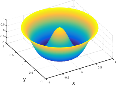
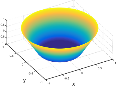
Figure 2. Example 5.1, left: plot of $f$; right: plot of $u_{\varepsilon}$ for $h=2^{-6}$.

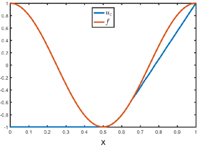
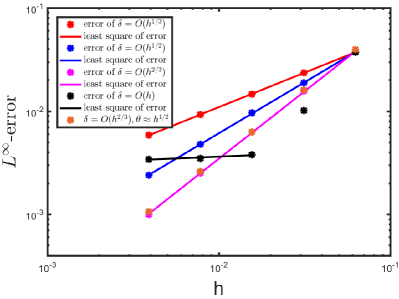
Figure 3. Example 5.1. Left: slice of numerical solution $u_{\varepsilon}$ on $\{(x,0):x\geq 0\}$ with $h=2^{-6},\delta=0.25h^{1/2},\theta\approx 0.25h^{1/2}$. Right: experimental rates of convergence upon choosing $\theta\approx 0.25h^{1/2}$ and $\delta=O(h^{\alpha})$ with $\alpha=1/3,1/2,2/3,1$. A least square regression is performed for $h^{-k}$ with $k=6,7,8$ and the case $\delta=O(h)$. The orders are about $0.67,0.99,1.30,0.07$. We also plot the errors for $\theta\approx h^{1/2},\delta=h^{2/3}$, and the errors are very close to choosing $\theta\approx 0.25h^{1/2},\delta=h^{2/3}$.

Example 5.2 (Lipschitz regularity $u\in C^{0,1}(\overline{\Omega})$).

Let $\Omega=\{x\in\mathbb{R}^{2}:|x|<1\}$ and

$$f(x)=\left\{\begin{array}[]{ll}1-4|x|,&0\leq|x|<1/4\\ 4|x|-1,&1/4\leq|x|<1/2\\ 2-2|x|,&1/2\leq|x|<3/4\\ 2|x|-1,&3/4\leq|x|\leq 1,\end{array}\right.\qquad u(x)=\left\{\begin{array}[]{ll}0,&0\leq|x|<1/4\\ |x|-1/4,&1/4\leq|x|<3/4\\ 2|x|-1,&3/4\leq|x|\leq 1.\end{array}\right.$$

This example deals with $f,u\in C^{0,1}(\overline{\Omega})$, i.e. both $f$ and $u$ are Lipschitz. The contact set $\mathcal{C}(f)$ consists of two disjoint components $\{x\in\mathbb{R}^{2}:|x|\geq 3/4\}$ and $\{x\in\mathbb{R}^{2}:|x|=1/4\}$. See Figure 4 (left) that displays slices on $\{(x,0):0\leq x\leq 1\}$ of $f,u$ and the numerical solution $u_{\varepsilon}$ with $h=2^{-6},\delta=0.25h^{1/2},\theta\approx 0.25h^{1/2}$. We point out that the pointwise error is very small in the regions $\{x\in\mathbb{R}^{2}:|x|\geq 3/4\}$ and $\{x\in\mathbb{R}^{2}:|x|\leq 1/4\}$; in the latter $u$ is linear and thus the interpolation error disappears. On the other hand, in the region $\{x\in\mathbb{R}^{2}:1/4<|x|<3/4\}$, where $u$ is only linear in the radial direction, we observe larger error for $u_{\varepsilon}$. Experimental convergence rates for different choices of $\delta=O(h^{\alpha})$ are plotted in Figure 4 (right): we see that these rates are better than those predicted in 3.8 (convergence rate). This theoretical rate can be improved upon exploiting that both functions $f$ and $u$ are non-smooth only at $\{0\}$ and across the curves $\{|x|=1/4\}$ and $\{|x|=3/4\}$. In fact, for those $x_{i}\in\mathcal{N}_{h}^{0}$ satisfying $\big{|}|x_{i}|-1/4\big{|}\leq\delta$ or $\big{|}|x_{i}|-3/4\big{|}\leq\delta$, according to 3.3 (consistency for $u$ with Hölder regularity), we have

$$T_{\varepsilon}[\mathcal{I}_{h}u;f](x_{i})\leq f(x_{i})-u(x_{i})\leq C(u)\delta,$$

whereas for the rest of $x_{i}\in\mathcal{N}_{h}^{0}$ the consistency error can be estimated exactly as for $f,u\in C^{1,1}(\overline{\Omega})$. Therefore carrying out the same analysis as in 3.7 (error estimate), we end up with the error estimate

$$\|u-u_{\varepsilon}\|_{L^{\infty}(\Omega_{h})}\leq C(u)\left(\delta+\frac{(\delta\theta)^{2}+h^{2}}{\delta^{2}}\right).$$

This yields a rate $O(h^{2/3})$ provided $\delta=O(h^{2/3})$, which is twice better than the rate from 3.8 but still worse than the experimental ones in Figure 4 (right).

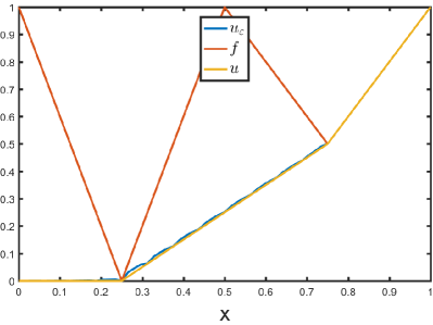
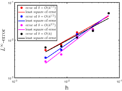
Figure 4. Example 5.2. Left: slices of $f,u$ and numerical solution $u_{\varepsilon}$ on $\{(x,0):x\geq 0\}$ with $h=2^{-6},\delta=0.25h^{1/2},\theta\approx 0.25h^{1/2}$. Right: experimental rates of convergence upon choosing $\theta=O(h^{1/2})$ and $\delta=O(h^{\alpha})$ with $\alpha=1/3,1/2,2/3,1$. The orders are about $0.78,0.96,1.06,0.74$.

Example 5.3 (Lipschitz $u\in C^{0,1}{(\overline{\Omega})}$ and nonstrictly convex $\Omega$).

Let $\Omega=(-1,1)^{2}$ and $f,u$ be as in [19, Example 6.3] with $\alpha=\beta=1$, i.e.

$$f(x,y)=xy\;,\qquad u(x,y)=|x+y|-1.$$

We point out that the Dirichlet boundary condition $u=f$ is attained on $\partial\Omega$ although the domain $\Omega$ is not strictly convex, whence 3.7 (error estimates) still applies. In this example, $f$ is smooth but $u$ is only Lipschitz because $\Omega$ is not uniformly convex and non-smooth: $u$ exhibits a kink across the diagonal $\{(x,y):x+y=0\}$ and is piecewise linear otherwise. Moreover, $u<f$ in $\Omega$ whence the contact set $\mathcal{C}(f)$ reduces to $\partial\Omega$.

Figure 5 (left) displays slices on $\{(x,y):x\geq 0,\ y=x\}$ of $f,u$ and the numerical solution $u_{\varepsilon}$ with $h=2^{-6},\delta=h^{1/2},\theta\approx 0.25h^{1/2}$. One can observe a clear mismatch between $u_{\varepsilon}$ and $u$ near the singular set $\{(x,y):x+y=0\}$. Compared with Example 5.1 (full regularity $u\in C^{1,1}(\overline{\Omega})$), the lack of regularity of $u$ here entails larger consistency error and $L^{\infty}$ error between $u_{\varepsilon}$ and $u$. Experimental convergence rates for different choices of $\delta=O(h^{\alpha})$ are depicted in Figure 5 (right); we see that the best convergence rate $O(h^{0.58})$ is found when $\delta=O(h^{1/3})$, which is again better than the $O(h^{1/3})$ rate predicted in 3.8 (convergence rate).

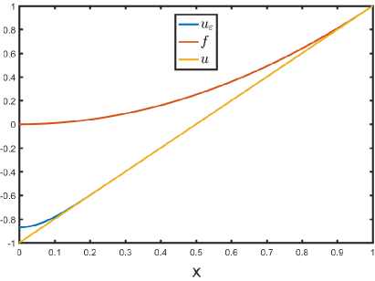
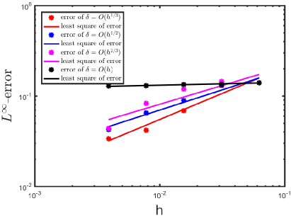
Figure 5. Example 5.3. Left: slice of numerical solution $u_{\varepsilon}$ on $\{(x,y):x\geq 0,\ y=x\}$ with $h=2^{-6},\delta=h^{1/2},\theta\approx 0.25h^{1/2}$. Right: experimental rates of convergence upon choosing $\theta=O(h^{1/2})$ and $\delta=O(h^{\alpha})$ with $\alpha=1/3,1/2,2/3,1$. The orders are about $0.58,0.45,0.41,0.03$.

Example 5.4 (non-attainment of Dirichlet condition).

Let $\Omega=(-1,1)^{2}$ and the function $f$ be $f(x,y)=\cos(\pi x)\cos(\pi y)$, whose restriction to $\partial\Omega$ is not convex. According to our definition (1.1), the convex envelope is given by

$$u(x,y)=\begin{cases}-1&\quad|x|+|y|\leq 1\\ -\cos\big{(}\pi(|x|+|y|-1)\big{)}&\quad 1<|x|+|y|\leq 1+\beta_{*}\\ -\cos\left(\pi\beta_{*}\right)+\pi\sin\left(\pi\beta_{*}\right)\big{(}|x|+|y|-1-\beta_{*}\big{)}&\quad 1+\beta_{*}<|x|+|y|,\end{cases}$$

where the constant $\beta_{*}\approx 0.2580$ satisfies the equation

$$-\cos(\pi\beta_{*})+\pi\sin(\pi\beta_{*})(1-\beta_{*})=1.$$

This assertion requires a brief explanation. First of all note that by symmetry it suffices to examine the first quadrant $0\leq x,y\leq 1$. On the edges $\{y=1\}$ and $\{x=1\}$ the function $u$ is convex by construction and definition of $\beta_{*}$; see Figure 6 (left). Since $u$ is flat along lines $x+y=\beta$ and convex along perpendicular lines, we infer that $u$ is convex. It remains to show that $u\leq f$ and $\geq$ than the convex envelope. To this end, we take convex combinations of boundary values $u(\beta-1,1)$ and $u(1,\beta-1)$ along the line $x+y=\beta$ with $1\leq\beta\leq 2$ and show that they are $\leq f(x,y)$. For $\beta=1$ we realize that $u(x,y)=-1\leq f(x,y)$ on $x+y=1$ and by symmetry for all $x+y\leq 1$. For $\beta>1$ a tedious calculation gives $u(x,y)=u(\beta-1,1)\leq f(\beta-1,1)\leq f(x,y)$ along $x+y=\beta$ as desired. We finally point out that the contact set $\mathcal{C}(f)$ consists of four boundary segments of length $2\beta_{*}$ centered at $(0,\pm 1),(\pm 1,0)$ and the four vertices $(\pm 1,\pm 1)$ of $\Omega$; see Figure 6 (left).

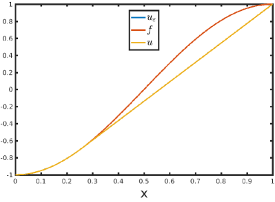
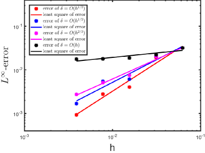
Figure 6. Example 5.4. Left: slices $f,u$ and $u_{\varepsilon}$ on the set $\{(x,1):x\geq 0\}$ with $h=2^{-6},\delta=2h^{1/2},\theta\approx 0.5h^{1/2}$. Note that $u_{\varepsilon}$ is indistinguishable from $u$ on this part of $\partial\Omega$. Right: experimental rates of convergence upon choosing $\theta=O(h^{1/2})$ and $\delta=O(h^{\alpha})$ with $\alpha=1/3,1/2,2/3,1$; the orders of convergence are about $1.30,1.04,0.91,0.20$.

We implemented the modified two-scale method (3.18), which first solves boundary subproblems on each edge of $\partial\Omega$ to find the trace of the discrete convex envelope $u_{\varepsilon}$ and next determines $u_{\varepsilon}$ within $\Omega$. Figure 6 (left) shows $f,u$ and $u_{\varepsilon}$ on the boundary set $\{(x,1):0\leq x\leq 1\}$; we point out that $u(x,1)=f(x,1)$ for $|x|\leq\beta_{*}$. Figure 6 (right) displays the $L^{\infty}$ error for several choices of $h$ and $\delta$: we see that the experimental convergence rate is about $O(h)$ for $\delta=O(h^{1/2})$, in agreement with theory, but the rates for $O(h^{\alpha})$ with $\alpha=1/3,2/3$ seem to be better than those predicted in 3.8 (convergence rate).

5.3. Computational performance

Thanks to the search tools provided by FELICITY [27, 28], the process of locating the triangle of the mesh containing points $x_{i}\pm\delta_{i}v_{j}$ and computing the barycentric coordinates only takes a small percentage of the total computing time; this is consistent with the two-scale method for the Monge-Ampère equation in [14]. In Example 5.1 for $h=2^{-6},\delta=0.25h^{1/2},\theta\approx 2h^{1/2}$, this process is 6.7% ($<$ 4 sec) of the total computation time (56.2 sec). The most time consuming part of the experiment is constructing and solving the linear systems, i.e. the third line in Algorithm 1; this takes 53.2% of the total time. We do not attempt to exploit the sparsity pattern of the matrix $B^{\bm{\alpha}}$ and simply resort to MATLAB backslash command for solving linear systems; we leave this important issue open. All of our computations are performed on an Intel Xeon E5-2630 v2 CPU (2.6 GHz), 16 GB RAM using MATLAB R2016b.

5.4. Comparison with other existing methods

In this subsection, we briefly compare our two-scale method with two other methods for the computation of convex envelopes: the wide stencil method in [19] and the modified version of Dolzmann’s method in [2]. Both the wide stencil method and our two-scale method are derived from the PDE formulation (1.3), and have a discrete operator with similar structure. As explained in Section 4, the wide stencil method can be viewed as a two-scale method with no interpolation error but with the constraint $\theta\approx h/\delta$. Our two-scale method suffers from the interpolation error but allows some freedom in the choice of parameters and works well on unstructured grids, which provide geometric flexibility to fit the boundary $\partial\Omega$.

The modified version of Dolzmann’s method in [2], built for the computation of rank-one convex envelopes of functions defined on $\mathbb{R}^{n\times m}$, can be applied to compute the convex envelope by simply letting $m=1$. When applied to compute convex envelopes, the technique of [2] hinges on the following algorithm: if $f^{(0)}=f$, and $f^{(k)}$ for $k\geq 1$ is iteratively defined as

(5.2) $$f^{(k)}(x)=\inf\{ \lambda f^{(k-1)}(x_{1})+(1-\lambda)f^{(k-1)}(x_{2}):$$

$$\lambda\in[0,1],x_{1},x_{2}\in\mathbb{R}^{d},\lambda x_{1}+(1-\lambda)x_{2}=x\},$$

then the convex envelope $u=f^{(d)}$ by Carathéodory’s theorem. Consequently, at the continuous level this process terminates in at most $d$ iterations. The method in [2] is a discrete version of this iteration on a structured grid $h\mathbb{Z}^{d}$ with interpolation on the finer grid $h^{2}\mathbb{Z}^{d}$, namely $x\in h\mathbb{Z}^{d}$ but $x_{1},x_{2}\in h^{2}\mathbb{Z}^{d}$ in (5.2). This is thus a two-scale method, with coarse scale $h$, but conceptually different from ours because it does not solve a PDE but rather an algebraic iteration. Moreover, it assumes $u=f$ in a layer $\{x\in\Omega:\textrm{dist}(x,\partial\Omega)\leq Ch\}$ near the boundary $\partial\Omega$ to deal with nodes in this region.

Regarding convergence rates, both the method in [2] and our two-scale method exhibit provable linear rates with respect to the coarse scale for solutions $u\in C^{0,1}(\overline{\Omega})$ according to Remark 3.9 (two important scenarios); moreover, Remark 3.9 also shows that our method is quadratic in the coarse scale $\delta$ and linear in the fine scale $h$ for $u\in C^{1,1}(\overline{\Omega})$ . Performing $d$ iterations of the discrete version of (5.2) is enough for linear convergence, whereas those for Howard’s method cannot be quantified a priori. However, practice reveals that $10$ iterations of Howard’s method are enough for convergence, which is consistent with its superlinear structure. Our iterations are simpler than those in [2] because they require much fewer interpolation points. Finally, our two-scale method is designed to work on unstructured meshes and deal with the Dirichlet boundary condition in a natural fashion. The boundary layer effect is handled via discrete barrier functions.

References

- [1] G. Barles and P. Souganidis, Convergence of approximation schemes for linear second order equations, Asymptot. Anal. 4(3):271–283, 1991.
- [2] S. Bartels, Linear convergence in the approximation of rank-one convex envelopes, ESAIM Math. Model. Numer. Anal. 38(5):811–820, 2004.
- [3] O. Bokanowski, S. Maroso, H. Zidani, Some convergence results for Howard’s algorithm, SIAM J. Numer. Anal. 47(4):3001–-3026, 2009.
- [4] S. C. Brenner and L. R. Scott, The Mathematical Theory of Finite Element Methods, Springer, 2007.
- [5] L. Caffarelli, L. Nirenberg and J. Spruck , The Dirichlet problem for the degenerate Monge-Ampère equation, Rev. Mat. Iberoam. 2(1):19–27, 1986.
- [6] G. De Philippis and A. Figalli, Optimal regularity of the convex envelope, Trans. Amer. Math. Soc. 367(6):4407–4422, 2015.
- [7] G. Dolzmann, Numerical computation of rank-one convex envelopes, SIAM J. Numer. Anal. 36(5):1621–1635, 1999.
- [8] G. Dolzmann and N. J. Walkington, Estimates for numerical approximations of rank one convex envelopes, Numer. Math. 85(4):647–663, 2000.
- [9] X. Feng and M. Jensen, Convergent semi-Lagrangian methods for the Monge-Ampère equation on unstructured grids form, SIAM J. Numer. Anal. 55(2):691–712, 2017.
- [10] C. E. Gutierrez, The Monge-Ampère Equation, Birkhäuser, 2016.
- [11] M. Hintermuller, K. Ito, and K. Kunisch, The primal-dual active set strategy as a semismooth Newton method, SIAM J. Optim., 13(3):865-–888, 2002.
- [12] M. Jensen and I. Smears, On the notion of boundary conditions in comparison principles for viscosity solutions, arXiv preprint arXiv:1703.07313.
- [13] W. Li and R. H. Nochetto, Optimal pointwise error estimates for two-scale methods for the Monge-Ampère equation, SIAM J. Numer. Anal. 56(3):1915–1941, 2018.
- [14] R. H. Nochetto, D. Ntogkas and W. Zhang, Two-scale method for the Monge-Ampère equation: convergence to the viscosity solution, Math. Comp. 88(316):637–664, 2019.
- [15] R. H. Nochetto, D. Ntogkas, and W. Zhang, Two-scale method for the Monge-Ampère equation: pointwise convergence rates, IMA J. Numer. Anal. doi:10.1093/imanum/dry026, 2018.
- [16] R. H. Nochetto and W. Zhang, Discrete ABP estimate and convergence rates for linear elliptic equations in non-divergence form, Found. Comp. Math. 18(3):537–593, 2017.
- [17] R. H. Nochetto and W. Zhang, Pointwise rates of convergence for the Oliker-Prussner method for the Monge-Ampère equation, Numer. Math. (to appear); arXiv:1611.02786.
- [18] A. M. Oberman, The convex envelope is the solution of a nonlinear obstacle problem, Proc. Amer. Math. Soc. 135(6):1689–1694, 2007.
- [19] A. M. Oberman, Computing the convex envelope using a nonlinear partial differential equation, Math. Models Meth. Appl. Sci, 18(05):759–780, 2008.
- [20] A. M. Oberman and Y. Ruan, A partial differential equation for the rank one convex envelope, Arch. Ration. Mech. Anal. 224(3):955–984, 2017.
- [21] A. M. Oberman and L. Silvestre, The Dirichlet problem for the convex envelope, Trans. Amer. Math. Soc. 363(11):5871–5886, 2011.
- [22] M. L. Puterman and S. L. Brumelle, On the convergence of policy iteration in stationary dynamic programming, Math. Oper. Res., 4(1):60–-69, 1979.
- [23] R. T. Rockafellar, Convex Analysis, Princeton University Press, 2015.
- [24] I. Smears and E. Süli, Discontinuous Galerkin finite flement approximation of Hamilton–Jacobi–Bellman equations with Cordes coefficients, SIAM J. Numer. Anal., 52(2):993–-1016, 2014.
- [25] N. S. Trudinger and J. I. Urbas, On second derivative estimates for equations of Monge-Ampère type, B. Aust. Math. Soc. 30(3):321–334, 1984.
- [26] M. Ulbrich, Semismooth Newton Methods for Variational Inequalities and Constrained Optimization Problems in Function Spaces, SIAM, vol 11, 2011.
- [27] S. W. Walker, FELICITY: A Matlab/C++ Toolbox for Developing Finite Element Methods and Simulation Modeling, SIAM J. Sci. Comput. 40(2):C234–C257, 2018.
- [28] S. W. Walker, FELICITY: Finite ELement Implementation and Computational Interface Tool for You, http://www.mathworks.com/matlabcentral/fileexchange/31141-felicity.