Breaking the Area Law: The Rainbow State

Abstract

An exponential deformation of a 1D critical Hamiltonian, with couplings falling on a length scale $h^{-1}$, gives rise to ground states whose entanglement entropy follows a volume law, i.e. the area law is violated maximally. The ground state is now in the so-called rainbow phase, where valence bonds connect sites on the left half with their symmetric counterparts on the right. Here we discuss some of the most relevant features of this rainbow phase, focusing on the XX and Heisenberg models. Moreover, we show that the rainbow state can be understood either as a thermo-field double of a conformal field theory with a temperature proportional to $h$ or as a massless Dirac fermion in a curved spacetime with constant negative curvature proportional to $h$. Finally, we introduce a study of the time-evolution of the rainbow state after a quench to a homogeneous Hamiltonian.

1 Introduction

Quantum many-body systems are models which allow us to illustrate important notions about macroscopic physics, e.g. magnetic behaviour, in terms of microscopic elementary interactions between the constituents of that system. In addition to their physical interest, the development of new methods for their study has given an impulse to other fields such as quantum integrability [1], quantum groups [2], quantum computation and information [3] or quantum simulators [4].

Early studies of many-body quantum mechanics used to make the assumption that each particle moves under the effective field created by all the others, i.e. Hartree-Fock or mean-field type methods [5]. These techniques are very successful to explain many properties of electrons in solids, through the use of the Fermi liquid approximation or Density Functional Theory [6, 7]. Nonetheless, they are unable to take completely into account the effect of strong correlations, which are a key in many magnetic properties of materials, superconductivity [8, 9], quantum Hall effect [10] or topological insulators [11].

Furthermore, the advent of new technologies such as cold atoms in optical lattices or trapped ions [12, 13], allows to engineer quantum systems in which strong correlations are not avoided, but looked for. The reasons can be to mimic other quantum systems or to harness the specific effects of quantum correlations to profit from them, building better computation and communication technologies.

Quantum entanglement is defined as the property of those pure states which do not allow a description as product states, i.e. non-factorizable states. For a composite system divided in two parts $A$ and $B$ with Hilbert space $\mathcal{H}=\mathcal{H}_{A}\otimes\mathcal{H}_{B}$, a factorizable state can be written as $\left|\psi\right\rangle=\left|\psi_{A}\right\rangle\otimes\left|\psi_{B}\right\rangle$, where states $\left|\psi_{A}\right\rangle$ and $\left|\psi_{B}\right\rangle$ describe $A$ and $B$ respectively. Factorizability of states can be determined using the Schmidt decomposition [14], all states in $\mathcal{H}$ can be expressed as

$$\left|\psi\right\rangle=\sum_{i=1}^{\chi}\lambda_{i}\left|a_{i}\right\rangle\otimes\left|b_{i}\right\rangle\;,$$

where $\left|a_{i}\right\rangle$ and $\left|b_{i}\right\rangle$ are orthonormal states of $\mathcal{H}_{A}$ and $\mathcal{H}_{B}$ respectively, and the Schmidt coefficients $\lambda_{i}\in\mathbf{R}^{+}$ and $\sum_{i}\lambda_{i}=1$. The Schmidt number (or Schmidt rank) $\chi$ is bounded by the dimension of Hilbert spaces of $A$ and $B$, i.e. $\chi\leq\min\{\dim\{\mathcal{H}_{A}\},\dim\{\mathcal{H}_{B}\}\}$. A state is factorizable if $\chi=1$, and if $\chi>1$ the state is entangled.

Factorizability defines absence of entanglement. In order to quantify entanglement it is convenient to consider an observer which is only allowed to access subsystem $A$. Even when the global state is pure, $\left|\psi\right\rangle$, the subsystem accessible to $A$ can be mixed. Thus, its quantum-mechanical description is performed via a reduced density matrix $\rho_{A}=\mathrm{Tr}_{\bar{A}}\left|\psi\right\rangle\!\!\left\langle\psi\right|$, where $\bar{A}$ is the complementary of subsystem $A$. We define the von Neumann’s entropy of this reduced density matrix

$$S_{A}=-\mathrm{tr}\,\{\rho_{A}\log{\left(\rho_{A}\right)}\}\;.$$

Let us remark that for a pure state, $S_{A}=S_{B}$. The von Neumann’s entropy satisfies $S_{A}\geq 0$, with $S_{A}=0$ only for factorizable states. Von Neumann’s entropy is also called the entanglement entropy (EE).

Why is $S_{A}$ called an entropy? There is a deep relation with the concept of entropy in statistical mechanics and information theory. Indeed, von Neumann’s entropy is a quantum analogue of Gibbs entropy. But in contrast, it is not related to thermal fluctuations. The EE can be argued to measure quantum correlations between subsystems. In classical information theory, the action of sending a message is also viewed as the action of correlating the sender and the receiver. The average amount of information contained in that message is measured with Shannon’s entropy [15]. Von Neumann’s entropy is just Shannon’s entropy of the eigenvalues of the reduced density matrix, which can be regarded as a probability distribution. Quantum information theory builds upon this deep relation between entanglement and information.

The goal of this paper is to present some details of the rainbow model and then to summarise some results previously obtained. This work is organised as follows. First we present the rainbow model and some details of the concentric valence bond states. After that, we present a summary of the results previously obtained, we include the references where more details were discussed.

2 Concentric Valence Bond States

Consider a spinless fermion chain of $L$ sites, whose dynamics is described by the Hamiltonian

$$H=-\sum_{i=1}^{L}t_{i}\;c^{\dagger}_{i}c_{i+1}+\mathrm{h.c.}$$ (1)

where $t_{i}$ represents the hopping amplitudes between sites $i$ and $i+1$, $c_{i}^{\dagger}$ and $c_{i}$ are, respectively, the fermionic creation and annihilation operators on site $i$, which satisfy anticommutation relations: $\{c_{j},c^{\dagger}_{k}\}=\delta_{jk}$, $\{c_{j},c_{k}\}=\{c_{j}^{\dagger},c^{\dagger}_{k}\}=0$.

Hamiltonian (1), which is quadratic in fermionic operators, is also called free fermion Hamiltonian. Moreover, free fermion Hamiltonians are solvable in terms of single-body states that are occupied by particles which move independently of each other. Diagonalising the hopping matrix, $T_{ij}=t_{i}(\delta_{j,i+1}+\delta_{j,i-1})$, $Tv_{k}=\epsilon_{k}v_{k}$, allows to obtain the single-body energy levels, $\epsilon_{k}$, and the single-body modes, $v_{k,i}$, which determine a canonical transformation

$$b^{\dagger}_{k}=\sum_{i}v_{k,i}c^{\dagger}_{i}\;,$$ (2)

where $v_{k,i}$ is an unitary matrix, thus the new operators $b^{\dagger}_{k}$ also follow fermionic commutation relations, i.e. $b_{k}$ are also fermionic operators.

All eigenstates of the Hamiltonian (1) have the form

$$\left|\psi\right\rangle=\prod_{k\in\Omega}b^{\dagger}_{k}\left|0\right\rangle\;,$$ (3)

where $\Omega$ is a subset of $\{1,\cdots,L\}$ denoting the occupied modes and $\left|0\right\rangle$ is the Fock vacuum, which is annihilated by the operators $c_{i}$. The energy for the state (3) is $E=\sum_{\Omega}\epsilon_{k}$. Therefore, the ground state (GS) is given by filling up all modes with lowest energy, i.e. $\Omega=\{k\mid\epsilon_{k}<0\}$. In absence of diagonal terms in the hopping matrix $T$, particle-hole symmetry forces $\epsilon_{k}=-\epsilon_{L+1-k}$, so the number of particles of the ground states is $|\Omega|=n_{F}=L/2$, i.e. we will operate at half-filling.

The correlation matrix, $C$, has elements defined by $C_{ij}\equiv\left\langle GS\right|c^{\dagger}_{i}c_{j}\left|GS\right\rangle$, which, in terms of the single-body modes is

$$C_{ij}=\sum_{k=1}^{n_{F}}\bar{v}_{k,i}v_{k,j}\;.$$ (4)

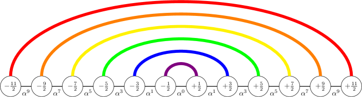
Figure 1: Rainbow state representation, showing the $(-k,+k)$ valence bonds above the central link. Each bond contributes as $\log(2)$ to the entanglement entropy, thus the entanglement entropy of the left (or right) half of the chain is $L\log 2$. The hopping amplitudes are given in terms of $\alpha=\exp(-h/2)$.

Let us now describe the family of local Hamiltonians whose GS approaches asymptotically the rainbow state. For bookkeeping convenience, let us number the sites as half-integers from $-(L-1)/2$ to $(L-1)/2$, and the corresponding links as integers, see Fig. 1. The rainbow Hamiltonian then reads

$$H\equiv-\frac{J}{2}c_{\frac{1}{2}}^{\dagger}c_{-\frac{1}{2}}-\frac{J}{2}\sum_{i=\frac{1}{2}}^{L-\frac{3}{2}}e^{-hi}\left[c^{\dagger}_{i}c_{i+1}+c^{\dagger}_{-i}c_{-(i+1)}\right]+\mathrm{h.c.}$$ (5)

where $h\in\mathbf{R}^{+}$ is the inhomogeneity parameter, and we may also define $\alpha\equiv\exp(-h/2$, as it is done in Fig. 1. Via the Jordan-Wigner transformation, this Hamiltonian is equivalent to the XX model for a spin-$1/2$ chain. For $h=0$ we recover the standard uniform 1D Hamiltonian of a spinless fermion model with open boundary conditions (OBC). Its low energy properties are captured by a conformal field theory (CFT) with central charge $c=1$: the massless Dirac fermion theory, or equivalently (upon bosonization) a Luttinger liquid with Luttinger parameter $K=1$.

For $h\gg 1$ we obtain the Hamiltonian used to illustrate a violation of the area law for local Hamiltonians [16]. On the other hand, for $h<0$ and truncating the chain to the sites $i>0$, one obtains a Hamiltonian which has the scale-free structure of Wilson’s approach to the Kondo impurity problem [17]. Models where $t_{i}$ is a hyperbolic function of the site index $i$ were considered in order to enhance the energy gap [18].

It is worth to notice the striking similarity between our system and the Kondo chain [19]. Indeed, let us divide our inhomogeneous chain into three parts: central link, left sites and right sites. The left and right sites correspond, in our analogy, to the spin up and down chains used in Wilson’s chain representation of the Kondo problem. In both cases, they form a system of free fermions, with exponentially decaying couplings. In the Kondo chain, notwithstanding, the central link becomes a magnetic impurity, which renders the full system non-gaussian.

3 Results

In a first paper [20] we analysed the deformation of the critical local 1D Hamiltonian to explore a smooth crossover between a log law and a volume law for the EE. We presented the details of the Heisenberg XX model. The value $h=0$ corresponds to the uniform model, which is described by the CFT, and in the $h\rightarrow\infty$ limit the GS becomes the rainbow state.

We used a graphical representation for the correlation matrix which operates as follows. For any matrix element, $C_{ij}$, we draw a line inside the unit circle with a colour which marks the strength of the correlation between those points. A finitely-correlated state will be characterised by a correlation matrix whose representation is given by short lines which do not go deep inside the unit circle. A conformal state, with infinite correlation length, is characterised by a certain self-similar structure in the geodesic pattern. Realisations of the rainbow state correlations are also very easy to spot. Figure 2 shows the structure of the correlation matrix for a 1D system with periodic boundary conditions (PBC) for a different systems. The intensity of each line connecting two sites is related to $\left|C_{ij}\right|$.

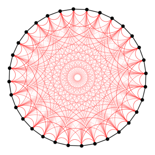
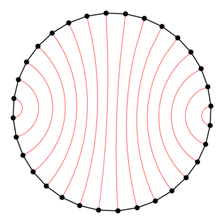
Figure 2: Structure of the correlation matrix defined by the elements $C_{ij}$ for a system of $N=32$ with periodic boundary conditions. Left: for a homogeneous system. Right: for a rainbow system.

We studied numerically the EE of blocks containing $\ell$ sites starting from the left extreme of the chain within the GS of Hamiltonian (5). For large values of $h$ we observe a characteristic tent shape in the EE, i.e. an approximately linear growth up to $\ell=L$ followed by a symmetric linear decrease, giving the volumetric behaviour. Figure 3 shows the EE for different values of $h$ for a system of $N=32$ sites. As the value of $h$ decreases, the slope decreases and ripples start to appear and for $h=0$ they recover the parity oscillations characteristics of the von Neumann entropy with OBC. For positive $h$, the slope was empirically shown to be given by $h/6$.

The analysis of the entanglement spectrum showed very interesting connections between conformal growth $S\sim\log(L)$ and volumetric growth $S\sim L$. Indeed, the spectrum is approximately equally spaced, with an entanglement spacing $\Delta L$ that decays with the system size as $1/\log(L)$ at the conformal point and as $1/L$ for rainbow system. We have also found that the EE is approximately proportional to the inverse of the entanglement spacing, in wide regions of the parameter space, which generalises previous known results for critical and massive systems.

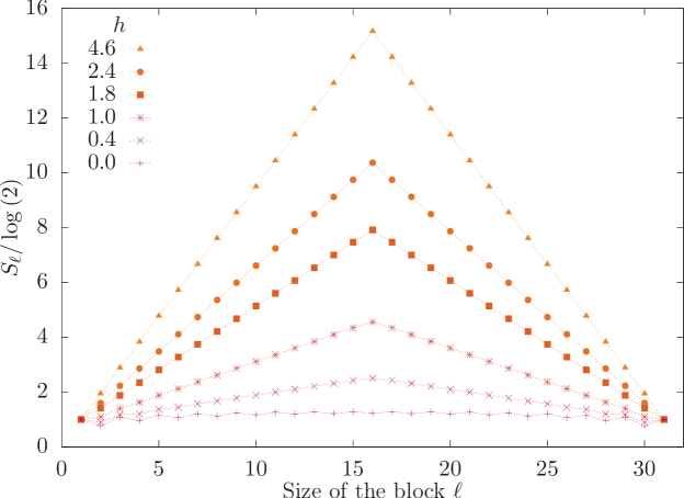
Figure 3: Block entropy $S_{\ell}$, for a system of size $L=16$ ($32$ sites). Notice the tent shape appear for small inhomogeneities in the system, denoting volumetric growth of the entanglement entropy.

In a second paper we have extended the analysis using field-theory methods [21]. We showed that the system can be described as a conformal deformation of the homogeneous case $h=0$, given by the following transformation

$$\tilde{x}=\mathrm{sign}(x)\frac{e^{h|x|}-1}{h}\;,$$ (6)

which maps the interval $x\in[-L,L]$ to $\tilde{x}\in[-\tilde{L},\tilde{L}]$, where $\tilde{L}=(e^{hL}-1)/h$.

If we expand the local operators $c_{n}$ into slow modes, $\psi_{R}(x)$ and $\psi_{L}(x)$ around the Fermi points $\pm k_{F}$

$$\frac{c_{n}}{\sqrt{a}}\simeq e^{ik_{F}x}\psi_{L}(x)+e^{-ik_{F}x}\psi_{R}(x)\;,$$ (7)

located at the position $x=an\in(-\mathcal{L},\mathcal{L})$, where $a$ is the lattice spacing and $\mathcal{L}=aL$ and, at half-filling $k_{F}=\pi/(2a)$ is the Fermi momentum. With this expansion we were able to obtain the Hamiltonian

$$H\simeq i\int_{-\tilde{L}}^{\tilde{L}}d\tilde{x}\left[\tilde{\psi}_{R}^{\dagger}\partial_{\tilde{x}}\tilde{\psi}_{R}-\tilde{\psi}_{L}^{\dagger}\partial_{\tilde{x}}\tilde{\psi}_{L}\right]\;,$$ (8)

which represents the free fermion Hamiltonian for a chain of length $2\tilde{L}$ under transformation (6) with the the fermion fields given by

$$\tilde{\psi}_{R,L}(\tilde{x})=\left(\frac{d\tilde{x}}{dx}\right)^{-1/2}\psi_{R,L}(x)\;.$$ (9)

Thus, using conformal invariance and substituting $L$ by $\tilde{L}$, we were able to transform the EE for a block of one-half of the critical system [22]

$$S^{CFT}_{L}=c\log(L)/6+c^{\prime}\;,$$ (10)

into the EE of the rainbow system

$$S_{L}=\frac{c}{6}\log{\left(\frac{e^{hL}-1}{h}\right)}+c^{\prime}\;,$$ (11)

which is shown in Figure 4 as a function of the half-chain size to check the theoretical prediction for different values of $h$.

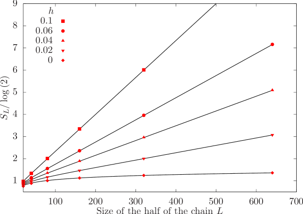
Figure 4: Comparing numerical results of the half-chain entropy of the rainbow system for different values of $h$ with the theoretical prediction.

We also showed that the corresponding conformal transformations suggests the definition of a temperature $T=1/\beta=h/(2\pi)$. Based on the entanglement spectrum, which is given the eigenvalues of the entanglement Hamiltonian

$$H_{E}=\sum_{p}\epsilon_{p}b^{\dagger}_{p}b_{p}+f_{0}\;,$$ (12)

where $b_{p}$ and $b^{\dagger}_{p}$ are fermion operators and the entanglement energies are given approximately by

$$\epsilon_{p}\simeq\Delta_{L}p,\quad\mathrm{for}\;p=\left\{\begin{array}[]{ll}\pm\frac{1}{2},\pm\frac{3}{2},\ldots,\pm\frac{L-1}{2},&L:\mathrm{even}\;,\\ 0,\pm 1,\pm 2,\ldots,\pm(L-2),&L:\mathrm{odd}\;,\end{array}\right.$$ (13)

where the level spacing $\Delta_{L}$ is related to the half-chain entropy. Moreover, the single-body entanglement energies fulfil

$$\epsilon_{p}\simeq\beta\epsilon^{CFT}_{p}=\left(\frac{2\pi}{h}\right)\left(\frac{\pi}{L}p\right)=\frac{2\pi^{2}}{z}p\;.$$ (14)

Thus, the appearance of a volume law entropy is linked to the existence of an effective temperature for the GS of the rainbow model that was finally identified with a thermo-field state

$$\left|\psi\right\rangle=\sum_{n}e^{-\beta E_{n}/2}\left|n\right\rangle_{L}\left|n\right\rangle_{R}\;,$$ (15)

where $\left|n\right\rangle_{R}$ and $\left|n\right\rangle_{L}$ correspond to the homogeneous GS for the right and left parts of the chain with $h=0$. This striking result points towards an unexpected connection with the theory of black holes and the emergence of space-time from entanglement. These intriguing connections were further explored within the framework of CFT [23]. Furthermore, we also showed how the deformation on the system accounts for the change in the dispersion relation, the single-particle wave functions in the vicinity of the Fermi point and the half-chain von Neumann and Rényi entropies. Finally, we show how to extend the rainbow Hamiltonian to more dimensions in a natural way and we to checked that the EE of the 2D analogue grows as the area of the block.

In a third paper [24] we applied methods of 2D quantum field theory in curved space-time to determine the entanglement structure of the rainbow phase. We showed that the rainbow system can be described by a massless Dirac fermion on a Riemannian manifold with constant negative curvature everywhere except at the centre, equivalent to a Poincaré metric with a strip removed. We used this identification to apply CFT for inhomogeneous 1D quantum systems [25] to provide accurate predictions for the smooth part of the $n$-order Rényi EE for blocks of different types such as the block at the chain’s edge given by the bipartition $A=[-L,x]$, $B=[x,L]$

$$S^{CFT}_{n}(x)=\frac{n+1}{12n}\ln{Y(x)}\;,$$ (16)

where

$$Y(x)=8e^{-h|x|}\frac{e^{hL}-1}{\pi L}\cos{\left(\frac{\pi}{2}\frac{e^{h|x|}-1}{e^{hL}-1}\right)}\;,$$ (17)

or for a block at an arbitrary position given by the bipartition $A=[x_{1},x_{2}]$, $B=[-L,x_{1}]\cup[x_{2},L]$

$$S^{CFT}_{n}(x_{1},x_{2})=\frac{n+1}{12n}\ln{4Y(x_{1},x_{2})}+E_{n}\;,$$ (18)

where $E_{n}$ is a non-universal constant, and with $e^{\sigma}=e^{-h|x|}$ we have

$$Y(x_{1},x_{2})=\frac{e^{\sigma(x_{1})+\sigma(x_{2})}\,16\tilde{L}^{2}}{\pi^{2}\cos{\left(\frac{\pi(\tilde{x}_{1}+\tilde{x}_{2})}{4\tilde{L}}\right)}}\sin{\left(\frac{\pi(\tilde{x}_{1}-\tilde{x}_{2})}{4\tilde{L}}\right)^{2}}\cos{\left(\frac{\pi\tilde{x}_{1}}{2\tilde{L}}\right)}\cos{\left(\frac{\pi\tilde{x}_{2}}{2\tilde{L}}\right)}\;.$$ (19)

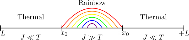
Figure 5: Illustration for the finite temperature behaviour of the rainbow chain. Let us find $x_{0}$ such that $T\approx J(x_{0})=J(-x_{0})$. Then, for $|x|>|x_{0}|$, $J(x)\ll T$ and the system behaves as if it were at infinite temperature. On the other hand, for $|x|<|x_{0}|$ the system behaves as if at zero temperature.

Furthermore, we also showed that for a physical temperature $T=J(x_{0})$, i.e. a temperature in the range of the energies spanned by the values of the hopping amplitude for a point $x_{0}\in[-L,L]$, the system splits into three regions: $x<-x_{0}$, $x\in[-x_{0},x_{0}]$ and $x>x_{0}$ (cf. Figure 5). The central region still behaves as if it were at $T=0$ while the two extremes as if they were at $T\rightarrow\infty$. Thus, the entropy of a block is obtained by adding the contributions on each region

$$S(x)\sim\left\{\begin{array}[]{ll}(L-|x|)\ln 2,&x\in(-L,-x_{0})\;,\\ (L-x_{0})\ln 2+(x_{0}-|x|)h/6,&x\in(-x_{0},x_{0})\;,\\ (L-2x_{0}+x)\ln 2,&x\in(x_{0},L)\;.\end{array}\right.$$ (20)

In a fourth paper [26], we study the time-evolution of the rainbow state and the dimer state, after a quench to a homogeneous Hamiltonian in 1D. The subsequent evolution of the EE presents very intriguing features. First, the EE of the half-chain of the rainbow decreases linearly with time and, after it reaches a minimal value, it increases again, eventually reaching (approximately) the initial state. Blocks of smaller sizes only decrease after a certain transient time, which can not be explained directly via a Lieb-Robinson bound [27], since the quench is global (cf. Figure 6).

The dimer state, on the other hand presents an opposite behaviour: the EE grows linearly for all blocks, reaching a maximally entangled state which resembles the rainbow state. Afterwards, the EE decreases again, cyclically. We also focus on the correlation between pairs of sites which suggests the motion of quasiparticles. Thus, we will attempt a theoretical explanation in terms of an extension of the quasiparticle picture by Calabrese and Cardy [28].

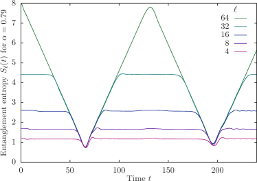
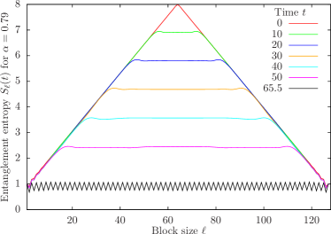
Figure 6: Time evolution of the entanglement entropy. Left: for blocks of size $\ell$ starting from the leftmost site. Notice the time periodicity and the strict order: the entropy of a larger block is always strictly larger than the entropy of a smaller one. Right: for the tent shape (cf. Fig. 3) of the entropy.

Acknowledgements. We would like to thank Pasquale Sodano for organising the conferences hosted at the International Institute of Physics (Natal) and for his efforts to collect the contributions for the Proceedings.

References

- [1] R. J. Baxter. Corner transfer matrices. Physica A., 106(1–2):18–27, 1981.
- [2] C. Gómez, M. Ruiz-Altaba, and G. Sierra. Quantum Groups in Two-Dimensional Physics. Cambridge Lecture Notes in Physics. Cambridge University Press, 1996.
- [3] M. A. Nielsen and I. L. Chuang. Quantum Computation and Quantum Information: 10th Anniversary Edition. Cambridge University Press, 10 edition, 2010.
- [4] M. Lewenstein, A. Sanpera, V. Ahufinger, B. Damski, A. Sen(De), and U. Sen. Ultracold atomic gases in optical lattices: mimicking condensed matter physics and beyond. Adv. Phys., 56(2):243–379, 2007.
- [5] N. W. Ashcroft and N. D. Mermin. Solid State Physics. Harcourt College Publishers, 1976.
- [6] P. Hohenberg and W. Kohn. Inhomogeneous Electron Gas. Phys. Rev., 136:B864–B871, Nov 1964.
- [7] W. Kohn and L. J. Sham. Self-Consistent Equations Including Exchange and Correlation Effects. Phys. Rev., 140:A1133–A1138, Nov 1965.
- [8] J. Bardeen, L. N. Cooper, and J. R. Schrieffer. Microscopic Theory of Superconductivity. Phys. Rev., 106:162–164, Apr 1957.
- [9] J. Bardeen, L. N. Cooper, and J. R. Schrieffer. Theory of Superconductivity. Phys. Rev., 108:1175–1204, Dec 1957.
- [10] R. B. Laughlin. Quantized Hall conductivity in two dimensions. Phys. Rev. B, 23:5632–5633, May 1981.
- [11] L. Fu and C. L. Kane. Topological insulators with inversion symmetry. Phys. Rev. B, 76:045302, Jul 2007.
- [12] I. Bloch, J. Dalibard, and W. Zwerger. Many-body physics with ultracold gases. Rev. Mod. Phys., 80:885–964, Jul 2008.
- [13] M. Lewenstein, A. Sanpera, and V. Ahufinger. Ultracold Atoms in Optical Lattices: Simulating quantum many-body systems. Oxford University Press, 2012.
- [14] E. Schmidt. Zur Theorie der linearen und nichtlinearen Integralgleichungen. Math. Ann., 63(4):433–476, 1907.
- [15] C.E. Shannon. A mathematical theory of communication. The Bell System Technical Journal, 27(3):379–423, July 1948.
- [16] G. Vitagliano, A. Riera, and J. I. Latorre. Volume-law scaling for the entanglement entropy in spin-1/2 chains. New J. Phys., 12(11):113049, 2010.
- [17] K. Okunishi and T. Nishino. Scale-free property and edge state of Wilson’s numerical renormalization group. Phys. Rev. B, 82:144409, Oct 2010.
- [18] H. Ueda, H. Nakano, K. Kusakabe, and T. Nishino. Scaling Relation for Excitation Energy under Hyperbolic Deformation. Progr. Theor. Phys., 124(3):389–398, 2010.
- [19] K. G. Wilson. The renormalization group: Critical phenomena and the Kondo problem. Rev. Mod. Phys., 47:773–840, Oct 1975.
- [20] G. Ramírez, J. Rodríguez-Laguna, and G. Sierra. From conformal to volume law for the entanglement entropy in exponentially deformed critical spin 1/2 chains. J. Stat. Mech., 2014(10):P10004, 2014.
- [21] G. Ramírez, J. Rodríguez-Laguna, and G. Sierra. Entanglement over the rainbow. J. Stat. Mech., 2015(6):P06002, 2015.
- [22] P. Calabrese and J. Cardy. Entanglement entropy and quantum field theory. J. Stat. Mech., 2004:P06002, 2004.
- [23] E. Tonni, J. Rodriguez-Laguna, and G. Sierra. Entanglement hamiltonian and entanglement contour in inhomogeneous 1D critical systems. J. Stat. Mech., 2018:043105, 2018.
- [24] J. Rodríguez-Laguna, J. Dubail, G. Ramírez, P. Calabrese, and G. Sierra. More on the rainbow chain: entanglement, space-time geometry and thermal states. J. Stat. Mech., 50(16):164001, 2017.
- [25] J. Dubail, J.-M. Stéphan, J. Viti, and P. Calabrese. Conformal Field Theory for Inhomogeneous One-dimensional Quantum Systems: the Example of Non-Interacting Fermi Gases. SciPost Phys., 2:002, 2017.
- [26] G. Ramírez, J. Rodríguez-Laguna, and G. Sierra. Quenched dynamics of valence bond states. Work in progress.
- [27] E. H. Lieb and D. W. Robinson. The finite group velocity of quantum spin systems. Commun. Math. Phys., 28(3):251–257, 1972.
- [28] P. Calabrese and J. Cardy. Evolution of entanglement entropy in one-dimensional systems. J. Stat. Mech., 2005(04):P04010, Apr 2005.