Optimal User Pairing for Achieving Rate Fairness in Downlink NOMA Networks

Abstract

In this paper, a downlink non-orthogonal multiple access (NOMA) network is studied. We investigate the problem of jointly optimizing user pairing and beamforming design to maximize the minimum rate among all users. The considered problem belongs to a difficult class of mixed-integer nonconvex optimization programming. We first relax the binary constraints and adopt sequential convex approximation method to solve the relaxed problem, which is guaranteed to converge at least to a locally optimal solution. Numerical results show that the proposed method attains higher rate fairness among users, compared with traditional beamforming solutions, i.e., random pairing NOMA and beamforming systems.

I Introduction

Non-orthogonal multiple access (NOMA) technique is being considered as a promising candidate of the fifth generation networks (5G) [1, 2]. By allowing multiple users to share the same time-frequency resources, NOMA adopts the successive interference cancellation (SIC) technique at users with better channel conditions that significantly improves the system performance in terms of the spectral efficiency and edge throughput of users with poorer channel conditions [3].

By following the principle of NOMA, two users with more distinct channel conditions should be paired [4]. Thus, the optimal user pairing is crucial to further improve the performance of NOMA systems. In particular, random user pairing schemes were proposed in [3, 4, 5, 6], where a near user is randomly paired with one farther from the base station (BS). Nonetheless, a general criteria for dynamic user pairing was not investigated. Recently, the optimal user pairing was studied in [7], where a minimum rate constraint for all NOMA users is additionally imposed. All of the aforementioned NOMA works focused on either single-antenna scenarios and/or random user pairing schemes. In the power domain NOMA, the BS should allocate a higher portion of transmission power to users with poor channel conditions from the viewpoint of fairness, which will generate strong interference to near users.

Motivated by the above discussion and shortcoming of the previous works, in this paper, we propose a dynamic user pairing and beamforming optimization problem for downlink (DL) NOMA systems from the perspective of fairness among users, which is inspired from the fact that the users with poor channel conditions may get a very low (even zero) throughput. The dynamic user pairing is done by introducing binary variables, which results in a difficult class of mixed-integer nonconvex optimization problem. The exhaustive search over all possible cases of user pairing provides the optimal performance of the considered problem but with prohibitive complexity. The main contributions of this paper are two-fold: $(i)$ We formulate a general optimization problem of dynamic user pairing and beamforming design, which has not been reported in the literature; $(ii)$ For efficient and practical implementations, we relax the binary constraints and propose a low-complexity iterative algorithm based on the inner approximation (IA) framework for its solution [8], which only solves a sequence of simple convex programs. Numerical results are provided to confirm that our proposed scheme is efficient in terms of the rate fairness.

Notation: Vectors are denoted by bold lower-case letters. $\mathbf{w}^{H}$, $\mathbf{w}^{T}$ and $\mathbf{w}^{*}$ are the Hermitian transpose, normal transpose and conjugate of a vector $\mathbf{w}$, respectively. $\mathbb{E}\{\cdot\}$ denotes the expectation and $\Re\{a\}$ returns the real part of a complex number $a$. $\mathbb{R}$ and $\mathbb{C}$ denote the set of all real and complex numbers, respectively. $\|\cdot\|$ denotes a vector’s Euclidean norm.

II System Model and Problem Formulation

II-A System Model

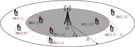
Figure 1: An illustration of DL NOMA consisting of one BS and ($M+N$) users.

We consider a downlink NOMA system consisting of one BS, a set of $M$ near users (UEs), denoted by $\mathcal{M}\triangleq\{1,2,\cdots,M\}$, and a set of $N$ far UEs, denoted by $\mathcal{N}\triangleq\{1,2,\cdots,N\}$, as illustrated in Fig. 1. In addition, $\mathtt{UE}(1,m)$ and $\mathtt{UE}(2,n)$ indicate the $m$-th UE with $m\in\mathcal{M}$ in inner-zone and the $n$-th UE with $n\in\mathcal{N}$ in outer-zone, respectively. For notational convenience, $\mathcal{G}\triangleq\{(1,1),\cdots,(1,M),(2,1),\cdots,(2,N)\}$ is defined as the set of all UEs. The BS is equipped with $L$ antennas while each user has a single antenna. Then, the received signal at $\mathtt{UE}(i,j)$ can be expressed as

$$y_{i,j} = \displaystyle\sum_{(i^{\prime},j^{\prime})\in\mathcal{G}}\mathbf{h}_{i,j}^{H}\mathbf{w}_{i^{\prime},j^{\prime}}{x}_{i^{\prime},j^{\prime}}+{n}_{i,j},\quad(i,j)\in\mathcal{G}\quad$$ (1)

where $\mathbf{h}_{i,j}\in\mathbb{C}^{L\times 1}$ and $\mathbf{w}_{i,j}\in\mathbb{C}^{L\times 1}$ are the channel vector from the BS to $\mathtt{UE}(i,j)$ and the beamforming vector, respectively. $x_{i,j}$ with $\mathbb{E}\{|x_{i,j}|^{2}\}=1$ and ${n}_{i,j}\sim\mathcal{CN}(0,\sigma^{2}_{i,j})$ are the transmitted symbol and the additive white Gaussian noise (AWGN) at $\mathtt{UE}(i,j)$, respectively.

In this paper, we assume that NOMA beamforming is exploited for pairs of two users, $\mathtt{UE}(1,m)$ and $\mathtt{UE}(2,n)$ $\forall m\in\mathcal{M},\forall n\in\mathcal{N}$. To do so, we introduce new binary variables $\alpha_{m,n}\in\{0,1\}$ as

$$\alpha_{m,n}=\left\{\begin{array}[]{ll}1,\quad\text{if}\ \mathtt{UE}(1,m)\ \text{and}\ \mathtt{UE}(2,n)\ \text{are paired,}\\ 0,\quad\text{otherwise}.\end{array}\right.$$ (2)

In each pair, the SIC technique will be adopted at $\mathtt{UE}(1,m)$ by following NOMA principle. In particular, $\mathtt{UE}(1,m)$ first decodes the message intended to $\mathtt{UE}(2,n)$ and subtracts it before decoding $\mathtt{UE}(1,m)$’s message. On the other hand, $\mathtt{UE}(2,n)$ will decode its own message directly by treating $\mathtt{UE}(1,m)$’s message as noise. By defining $\boldsymbol{\alpha}\triangleq{[\alpha_{m,n}]}_{m\in\mathcal{M},n\in\mathcal{N}}$, $\mathbf{w}_{1}\triangleq{[\mathbf{w}_{1,m}]}_{m\in\mathcal{M}}$, $\mathbf{w}_{2}\triangleq{[\mathbf{w}_{2,n}]}_{n\in\mathcal{N}}$ and $\mathbf{w}\triangleq{[\mathbf{w}_{1}^{H}\text{ }\mathbf{w}_{2}^{H}]^{H}}$, the signal-to-interference-plus-noise ratio (SINR) at $\mathtt{UE}(1,m)$ and $\mathtt{UE}(2,n)$ can be written as

$${\gamma_{1,m}}(\mathbf{w},\boldsymbol{\alpha}) = \frac{{{{\left|{\mathbf{h}_{{1,m}}^{H}{\mathbf{w}_{{1,m}}}}\right|}^{2}}}}{\Xi_{m}(\mathbf{w},\boldsymbol{\alpha})},$$ (3a)

$$\gamma_{2,n}(\mathbf{w},\boldsymbol{\alpha}) = \underset{m\in\mathcal{M}}{\min}\Bigl{\{}\frac{{\left|{\mathbf{h}_{{2,n}}^{H}{\mathbf{w}_{{2,n}}}}\right|}^{2}}{\Phi_{n}(\mathbf{w})},\frac{{\left|{\mathbf{h}_{{1,m}}^{H}{\mathbf{w}_{{2,n}}}}\right|}^{2}}{\alpha_{m,n}\Psi_{m,n}(\mathbf{w})}\Bigr{\}}\quad$$ (4a)

where $\Xi_{m}(\mathbf{w},\boldsymbol{\alpha})$, $\Phi_{n}(\mathbf{w})$ and $\Psi_{m,n}(\mathbf{w})$ are defined as

$$\Xi_{m}(\mathbf{w},\boldsymbol{\alpha}) = \displaystyle\sum_{m^{\prime}\in\mathcal{M}\backslash\{m\}}\left|\mathbf{h}_{1,m}^{H}\mathbf{w}_{1,m^{\prime}}\right|^{2}$$

$$+\displaystyle\sum_{n^{\prime}\in\mathcal{N}}(1-\alpha_{m,n^{\prime}})\left|\mathbf{h}_{1,m}^{H}\mathbf{w}_{2,n^{\prime}}\right|^{2}+\sigma_{1,m}^{2},$$

$$\Phi_{n}(\mathbf{w}) = \displaystyle\sum_{(i,j)\in\mathcal{G}\backslash\{(2,n)\}}\left|\mathbf{h}_{2,n}^{H}\mathbf{w}_{i,j}\right|^{2}+\sigma_{2,n}^{2},$$

$$\Psi_{m,n}(\mathbf{w}) = \displaystyle\sum_{(i,j)\in\mathcal{G}\backslash\{(2,n)\}}\left|\mathbf{h}_{1,m}^{H}\mathbf{w}_{i,j}\right|^{2}+\sigma_{1,m}^{2}.$$

In (4a), $\frac{{\left|{\mathbf{h}_{{2,n}}^{H}{\mathbf{w}_{{2,n}}}}\right|}^{2}}{\Phi_{n}(\mathbf{w})}$ and $\frac{{\left|{\mathbf{h}_{{1,m}}^{H}{\mathbf{w}_{{2,n}}}}\right|}^{2}}{\alpha_{m,n}\Psi_{m,n}(\mathbf{w})}$ are the SINRs of $\mathtt{UE}(2,n)$ decoded at $\mathtt{UE}(2,n)$ and $\mathtt{UE}(1,m)$, respectively. Clearly, if $\alpha_{m,n}=0,\ \forall m,n$, then $\gamma_{2,n}(\mathbf{w},\boldsymbol{\alpha})=\frac{{\left|{\mathbf{h}_{{2,n}}^{H}{\mathbf{w}_{{2,n}}}}\right|}^{2}}{\Phi_{n}(\mathbf{w})}$.

II-B Problem Formulation

From (3a), the achievable throughput for $\mathtt{UE}(i,j)$ can be derived as

$$R_{i,j}(\mathbf{w},\boldsymbol{\alpha})=\log_{2}(1+\gamma_{i,j}(\mathbf{w},\boldsymbol{\alpha})),\quad(i,j)\in\mathcal{G}.$$ (5)

Herein, we aim to maximize the minimum rate among all UEs, called max-min rate (MMR) for short. Accordingly, an optimization problem can be mathematically formulated as

$$\max\limits_{\mathbf{w},\boldsymbol{\alpha}}$$ min_(i,j)∈G R_i,j(w,α) (6a)

$${\mathrm{s.t.}}$$ ∥w∥^2 ≤P^max_BS, (7a)

where (7a) represents the transmit power constraint at the BS, $P_{\text{BS}}^{\text{max}}$ and constraints (LABEL:maxminratec), (LABEL:maxminrated), (LABEL:maxminratee) establish the criteria for user pairing. Specifically, constraints (LABEL:maxminrated) and (LABEL:maxminratee) ensure that each $\mathtt{UE}(i,j)$ can opportunistically pair to one UE only. We can see that (6a) is nonsmooth and nonconcave and (LABEL:maxminratec) corresponds to binary constraints, leading to a mixed-integer nonconvex optimization of problem (6a). Thus, problem (6a) is intractable and it may not be possible to convert the problem into an equivalent convex one. Following some recent studies on wireless communication system designs [9, 10], we aim at solving (6a) based on the application of IA method, which efficiently provides a locally optimal solution with low complexity.

III Proposed Iterative Algorithm

The main difficulty of solving (6a) is to handle the binary constraints (LABEL:maxminratec). To overcome this issue, we first relax $\alpha_{m,n}\in\{0,1\}$ to $0\leq\alpha_{m,n}\leq 1$ and rewrite (LABEL:maxminratec) as

$$\max\limits_{\mathbf{w},\boldsymbol{\alpha}}$$ min_(i,j)∈Gγ_i,j(w,α) (11a)

$${\mathrm{s.t.}}$$ 0≤α_m,n≤1, ∀m ∈M, ∀n∈N, (11b)

where the optimal solutions of MMR problem and max-min SINR problem are identical. We can observe that the feasible sets are convex (quadratic and linear constraints), and thus only the objective function (11a) remains nonconcave. In order to apply the IA method, we introduce a new variable $\beta$ to re-express (11) equivalently as

$$\max\limits_{\mathbf{w},\boldsymbol{\alpha},{\beta}}$$ 1/β (12a)

$${\mathrm{s.t.}}$$ 1/β≤γ_i,j, (i,j)∈G, (12b)

We remark that the equivalence between (11) and (12) is guaranteed due to the fact that constraints (12b) must hold with equality at optimum [10].

Concavity of (12a): The function $1/\beta$ is convex and thus its first order approximation at a feasible point $\beta^{(\kappa)}$ found at iteration $\kappa$ is given by

$$\frac{1}{\beta}\geq\frac{2}{\beta^{(\kappa)}}-\frac{\beta}{(\beta^{(\kappa)})^{2}}$$

which is a linear function.

Convexity of (12b): Here, we consider two cases of $i\in\{1,2\}$ due to different structures of the SINR functions.

($i$) With $i=1$: constraint (12b) is $1/\beta\leq\gamma_{1,j}$, which can be revised as

$$\Xi_{m}(\mathbf{w},\boldsymbol{\alpha})\leq\left|\mathbf{h}_{1,m}^{H}\mathbf{w}_{1,m}\right|^{2}\beta.$$ (13)

Next, we introduce new variables $\boldsymbol{\tau}\triangleq\{\tau_{m,n}\}_{m\in\mathcal{M},n\in\mathcal{N}}$ to decompose (13) into the following two constraints:

$$\eqref{ctSRNRzone1}\Leftrightarrow \left|\mathbf{h}_{1,m}^{H}\mathbf{w}_{2,n^{\prime}}\right|^{2}\leq\tau_{m,n^{\prime}}\ ,\ m\in\mathcal{M},n^{\prime}\in\mathcal{N},$$ (14aa)

$$\eqref{ctSRNRzone1}\Leftrightarrow \Xi_{m}(\mathbf{w},\boldsymbol{\alpha},\boldsymbol{\tau})\leq\left|\mathbf{h}_{1,m}^{H}\mathbf{w}_{1,m}\right|^{2}\beta\$$ (14ba)

where $\Xi_{m}(\mathbf{w},\boldsymbol{\alpha},\boldsymbol{\tau})=\displaystyle\sum_{m^{\prime}\in\mathcal{M}\backslash\{m\}}\left|\mathbf{h}_{1,m}^{H}\mathbf{w}_{1,m^{\prime}}\right|^{2}+\displaystyle\sum_{n^{\prime}\in\mathcal{N}}(1-\alpha_{m,n^{\prime}})\tau_{m,n^{\prime}}+\sigma_{1,m}^{2}.$ Since (14aa) is convex constraint, we only need to handle the non-convexity of (14ba). Constraint (14ba) is innerly convexified as

$$\widehat{\Xi}_{m}^{(\kappa)}(\mathbf{w},\boldsymbol{\alpha},\boldsymbol{\tau})\leq f_{1,m}^{(\kappa)}(\mathbf{w})\beta,\quad m\in\mathcal{M}.$$ (15)

where $\widehat{\Xi}_{m}^{(\kappa)}(\mathbf{w},\boldsymbol{\alpha},\boldsymbol{\tau})$ is a convex upper bound of $\Xi_{m}(\mathbf{w},\boldsymbol{\alpha},\boldsymbol{\tau})$ by using [10, Eq. (B.1)]:

$$\widehat{\Xi}_{m}^{(\kappa)}(\mathbf{w},\boldsymbol{\alpha},\boldsymbol{\tau})\triangleq\sum\limits_{m^{\prime}\in\mathcal{M}\backslash\{m\}}\left|\mathbf{h}_{1,m}^{H}\mathbf{w}_{1,m^{\prime}}\right|^{2}+\sigma_{1,m}^{2}+$$

$$\displaystyle\sum_{n^{\prime}\in\mathcal{N}}\Bigl{(}\frac{1}{2}\frac{1-\alpha_{m,n^{\prime}}^{(\kappa)}}{\tau_{m,n^{\prime}}^{(\kappa)}}\tau_{m,n^{\prime}}^{2}+\frac{1}{2}\frac{\tau_{m,n^{\prime}}^{(\kappa)}}{1-\alpha_{m,n^{\prime}}^{(\kappa)}}(1-\alpha_{m,n^{\prime}})^{2}\Bigr{)}$$

and $f_{1,m}^{(\kappa)}(\mathbf{w})$ is a lower bound of the convex function $\left|\mathbf{h}_{1,m}^{H}\mathbf{w}_{1,m}\right|^{2}$ given as [10, Eq. (22)]:

$${\left|\mathbf{h}_{1,m}^{H}\mathbf{w}_{1,m}\right|^{2}}\geq {2\Re\{(\mathbf{h}_{1,m}^{H}\mathbf{w}_{1,m}^{(\kappa)})^{H}(\mathbf{h}_{1,m}^{H}\mathbf{w}_{1,m})\}}$$

$$-{|\mathbf{h}_{1,m}^{H}\mathbf{w}_{1,m}^{(\kappa)}|^{2}}\quad\triangleq f_{1,m}^{(\kappa)}(\mathbf{w}).$$

($ii$) With $i=2$: constraint (12b) is replaced by

$$1/\beta\leq\frac{{|{\mathbf{h}_{{2,n}}^{H}{\mathbf{w}_{{2,n}}}}|}^{2}}{\Phi_{n}(\mathbf{w})},\quad\forall n\in\mathcal{N},$$ (16aa)

$$1/\beta\leq\frac{{|{\mathbf{h}_{{1,m}}^{H}{\mathbf{w}_{{2,n}}}}|}^{2}}{\alpha_{m,n}\Psi_{m,n}(\mathbf{w})},\quad\forall m\in\mathcal{M},\forall n\in\mathcal{N}.$$ (16ba)

Similarly to (14ba), constraints in (16ba) are innerly covexified as

$$\Phi_{n}(\mathbf{w})\leq f_{2,n}^{(\kappa)}(\mathbf{w})\beta,\quad\forall n\in\mathcal{N},$$ (17aa)

$$\Psi_{m,n}(\mathbf{w})\leq\tilde{f}_{m,n}^{(\kappa)}(\mathbf{w},\boldsymbol{\alpha})\beta,\quad\forall m\in\mathcal{M},\forall n\in\mathcal{N}$$ (17ba)

where $f_{2,n}^{(\kappa)}(\mathbf{w})$ is a lower bound of $|{\mathbf{h}_{{2,n}}^{H}{\mathbf{w}_{{2,n}}}}|^{2}$ given as:

$$f_{2,n}^{(\kappa)}(\mathbf{w})\triangleq{2\Re\{(\mathbf{h}_{2,n}^{H}\mathbf{w}_{2,n}^{(\kappa)})^{H}(\mathbf{h}_{2,n}^{H}\mathbf{w}_{2,n})\}}-{|\mathbf{h}_{2,n}^{H}\mathbf{w}_{2,n}^{(\kappa)}|^{2}}$$

and $\tilde{f}_{m,n}^{(\kappa)}(\mathbf{w},\boldsymbol{\alpha})$ is a lower bound of ${\left|{\mathbf{h}_{{1,m}}^{H}{\mathbf{w}_{{2,n}}}}\right|}^{2}/\alpha_{m,n}$ derived by using [10, Eq. (38)]:

$$\tilde{f}_{m,n}^{(\kappa)}(\mathbf{w},\boldsymbol{\alpha})\triangleq \frac{2\Re\{(\mathbf{h}_{1,m}^{H}\mathbf{w}_{2,n}^{(\kappa)})^{H}(\mathbf{h}_{1,m}^{H}\mathbf{w}_{2,n})\}}{\alpha_{m,n}^{(\kappa)}}$$

$$-\frac{|\mathbf{h}_{1,m}^{H}\mathbf{w}_{2,n}^{(\kappa)}|^{2}}{{(\alpha_{m,n}^{(\kappa)})}^{2}}(\alpha_{m,n}).$$

We should note that constraints (15) and (17ba) can be expressed as second-order cone (SOC) constraints, which are obviously convex ones.

Summing up, problem (11) can be approximated as the following convex program at iteration $(\kappa+1)$:

$$\max\limits_{\mathbf{w},\boldsymbol{\alpha},{\beta},\boldsymbol{\tau}}$$ η≜2β(κ) - β(β(κ))2 (18a)

$${\mathrm{s.t.}}$$ (7a), (LABEL:maxminrated), (LABEL:maxminratee),(11b), (14aa), (15), (17ba). (19a)

We have numerically observed that some values of $\alpha_{m,n}$ are very close to binary but not exactly binary values at the optimum. This makes (6a) infeasible. Therefore, we further introduce the rounding function after obtaining the optimal solution of problem (18a) as

$$\alpha_{m,n}^{\star}=\Big{\lfloor}\alpha_{m,n}^{(\kappa)}+\frac{1}{2}\Big{\rfloor},\quad m\in\mathcal{M},n\in\mathcal{N}.$$ (20)

The proposed algorithm is summarized in Algorithm 1. Specifically, Algorithm 1 consists of two phases: In phase 1, we successively solve (18a) to achieve $(\mathbf{w}^{(\star)},\boldsymbol{\alpha}^{(\star)},\beta^{(\star)},\boldsymbol{\tau}^{(\star)})$. In phase 2, we first use the rounding function (20) to force $\boldsymbol{\alpha}$ into the nearest Boolean values, and then resolve problem (18a) for a fixed value of $\boldsymbol{\alpha}$ to find the optimal solution $\mathbf{w}^{(\star)}$. Moreover, due to the fact that the IA method is employed, Algorithm 1 converges to a stationary point, which also satisfies the Karush-Kuhn-Tucker (KKT) conditions of (11). The detailed proof can be done by following the same steps in [8, 10].

0:  Set $\kappa=0$ and generate feasible initial points $(\mathbf{w}^{(0)},\boldsymbol{\alpha}^{(0)},{\beta}^{(0)},\boldsymbol{\tau}^{(0)})$.

0:  

1:  repeat

2:     Solve the convex program (18a) to compute the optimal solution $(\mathbf{w}^{\star},\boldsymbol{\alpha}^{\star},{\beta}^{\star},\boldsymbol{\tau}^{\star})$.

3:     Update  $(\mathbf{w}^{(\kappa+1)},\boldsymbol{\alpha}^{(\kappa+1)},{\beta}^{(\kappa+1)},\boldsymbol{\tau}^{(\kappa+1)})=(\mathbf{w}^{\star},\boldsymbol{\alpha}^{\star},{\beta}^{\star},\boldsymbol{\tau}^{\star})$.

4:     Set $\kappa=\kappa+1.$

5:  until Convergence

6:  Output-1: $(\mathbf{w}^{\star},{\beta}^{\star},\boldsymbol{\tau}^{\star})=(\mathbf{w}^{(\kappa)},{\beta}^{(\kappa)},\boldsymbol{\tau}^{(\kappa)})$,     $\boldsymbol{\alpha}^{\star}$ is updated by (20).

6:  

7:  Run steps 1- 5 again to find beamformers $\mathbf{w}$ with fixed $\boldsymbol{\alpha}$.

8:  Output-2: ($\mathbf{w}^{\star},\boldsymbol{\alpha}^{\star}$).

Algorithm 1 Proposed Iterative Algorithm to Solve (11)

Complexity analysis: Since problem (18a) has $x=(2(M+N)+3MN+1)$ quadratic and linear constraints and $y=L(M+N)+2MN+1$ optimization variables , the per-iteration complexity of solving (18a) is $\mathcal{O}\big{(}x^{2.5}(y^{2}+x)\big{)}$ [11].

IV Numerical Results

We consider a small-cell network serving 8 UEs with $M$ = 3 UEs in inner-zone and $N$ = 5 UEs in outer-zone. Other important parameters are included in Table I. Algorithm 1 is terminated when the increase in the objective value between two consecutive iterations is less than $10^{-3}$.

TABLE I: SIMULATION PARAMETERS

Parameters	Value
Bandwidth	20 [MHz]
Noise power density	-174 [dBm/Hz]
Path loss from the BS to a UE, $\sigma_{\mathsf{PL}}$	140 + 37.6$\log_{10}(d)$ [dB]
Shadowing standard deviation	8 [dB]
Radius of the cell $(R)$	100 [m]
Coverage of near UEs $(d)$	50 [m]
Distance between BS and the nearest UE	$\geq$ 5 [m]

Fig. 2 depicts the averaged MMR performance of our proposed algorithm (NOMA-Optimal) with two other resource allocation schemes as a function of $P_{\mathrm{BS}}^{\max}$. The solution of NOMA-Random [3] is found by using Algorithm 1 with $\alpha_{m,n}$ being randomly chosen. The results are averaged over 100 random channel realizations. As expected, the MMR of Algorithm 1 is higher than that of NOMA-Random and beamforming schemes, of which the gaps are about 0.5 bps/Hz and 1 bps/Hz, respectively. This further demonstrates the effectiveness of jointly optimizing user pairing and beaforming design.

In Fig. 3, we illustrate the convergence behavior of Algorithm 1 for different number of antennas at the BS. We can see that increasing the number of antennas $L$ requires more number of iterations to converge. Nevertheless, it requires a few iterations to achieve the optimal solution, i.e., about 17 iterations for $L=16$.

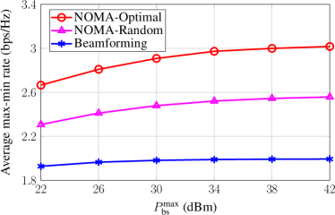
Figure 2: Average max-min rate performance versus $P_{\mathrm{BS}}^{\max}$ with $L=6$.

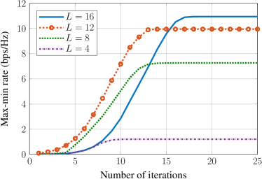
Figure 3: Convergence of Alg. 1 for one channel realization with $P_{\text{BS}}^{\text{max}}=30\text{dBm}$.

V Conclusions

This paper studied a DL NOMA network, where the optimal user pairing is investigated. We formulated a max-min rate optimization problem to jointly optimize user pairing and beamforming design, and then designed an efficient iterative algorithm based on the IA method to solve it. The effectiveness of the proposed algorithm has been demonstrated by the numerical results.

References

- [1] L. D. et al., “Non-orthogonal multiple access for 5G: Solutions, challenges, opportunities, and future research trends,” IEEE Commun. Mag., vol. 53, no. 9, pp. 74–81, Sept. 2015.
- [2] Y. L. et al., “Nonorthogonal multiple access for 5G and beyond,” Proce. IEEE, vol. 105, no. 12, pp. 2347–2381, Dec. 2017.
- [3] V.-D. Nguyen, H. D. Tuan, T. Q. Duong, H. V. Poor, and O.-S. Shin, “Precoder design for signal superposition in MIMO-NOMA multicell networks,” IEEE J. Select. Areas Commun., vol. 35, no. 12, pp. 2681–2695, Dec. 2017.
- [4] Z. Ding, P. Fan, and H. V. Poor, “Impact of user pairing on 5G nonorthogonal multiple-access downlink transmissions,” IEEE Trans. Veh. Technol., vol. 65, no. 8, pp. 6010–6023, Aug. 2016.
- [5] Z. Ding, F. Adachi, and H. V. Poor, “The application of MIMO to non-orthogonal multiple access,” IEEE Trans. Wireless Commun., vol. 15, no. 1, pp. 537–552, Jan. 2016.
- [6] X. Chen, F. Gong, G. Li, H. Zhang, and P. Song, “User pairing and pair scheduling in massive mimo-noma systems,” IEEE Commun. Lett., vol. 22, no. 4, pp. 788–791, Apr. 2018.
- [7] L. Zhu, J. Zhang, Z. Xiao, X. Cao, and D. O. Wu, “Optimal user pairing for downlink non-orthogonal multiple access (NOMA),” IEEE Wireless Commun. Lett., July 2018, Early access.
- [8] B. R. Marks and G. P. Wight, “A general inner approximation algorithm for nonconvex mathematical programms,” Operations Research, vol. 26, no. 4, pp. 681–683, July 1978.
- [9] V.-D. Nguyen, T. Q. Duong, H. D. Tuan, O.-S. Shin, and H. V. Poor, “Spectral and energy efficiencies in full-duplex wireless information and power transfer,” IEEE Trans. Commun., vol. 65, no. 5, pp. 2220–2233, May 2017.
- [10] V.-D. Nguyen, H. V. Nguyen, O. A. Dobre, and O.-S. Shin, “A new design paradigm for secure full-duplex multiuser systems,” IEEE J. Select. Areas Commun., vol. 36, no. 7, pp. 1480–1498, July 2018.
- [11] Y. Labit, D. Peaucelle, and D. Henrion, “SEDUMI INTERFACE 1.02: A tool for solving LMI problems with SEDUMI,” pp. 272–277, Oct. 2002.