Multivariate Arrival Times with Recurrent Neural Networks for Personalized Demand Forecasting

Abstract

Access to a large variety of data across a massive population has made it possible to predict customer purchase patterns and responses to marketing campaigns. In particular, accurate demand forecasts for popular products with frequent repeat purchases are essential since these products are one of the main drivers of profits. However, buyer purchase patterns are extremely diverse and sparse on a per-product level due to population heterogeneity as well as dependence in purchase patterns across product categories. Traditional methods in survival analysis have proven effective in dealing with censored data by assuming parametric distributions on inter-arrival times. Distributional parameters are then fitted, typically in a regression framework. On the other hand, neural-network based models take a non-parametric approach to learn relations from a larger functional class. However, the lack of distributional assumptions make it difficult to model partially observed data. In this paper, we model directly the inter-arrival times as well as the partially observed information at each time step in a survival-based approach using Recurrent Neural Networks (RNN) to model purchase times jointly over several products. Instead of predicting a point estimate for inter-arrival times, the RNN outputs parameters that define a distributional estimate. The loss function is the negative log-likelihood of these parameters given partially observed data. This approach allows one to leverage both fully observed data as well as partial information. By externalizing the censoring problem through a log-likelihood loss function, we show that substantial improvements over state-of-the-art machine learning methods can be achieved. We present experimental results based on two open datasets as well as a study on a real dataset from a large retailer.

I Introduction

Accurately predicting each customer’s behavior for each product is useful in direct marketing efforts which can lead to significant advantages for a retailer by driving increased sales, margin, and return on investment [13]. Of special interest are replenishable products such as regularly consumed food products (e.g. milk) or regularly replenished personal care products (e.g. soap). These products drive store traffic, basket size, and customer loyalty, which are of strategic importance in a highly competitive retail environment [22].

Traditional approaches to this problem defines customers to be “alive” if purchases were made. These models make assumptions on the distributions of purchase counts and lifetimes of individual customers as well as population heterogeneity [2, 29, 18, 6]. They can be framed in a Cox Proportional Hazards model where covariates are regressed as a multiplicative factor in a baseline hazard function [23]. Solving the maximum likelihood problem yields optimal distributional estimates that model these behaviors. In a scenario with sparse purchase data, this can be useful since non-purchases can reveal information about whether a customer is likely to make a purchase in the future.

However, these models impose strict assumptions such as independence and stationarity. Covariates are often modeled linearly, further restricting the space of possible functional relations that are possible. While these assumptions were essential for tractability purposes, they can no longer be taken for granted when we wish to model highly-correlated, high-dimensional and heterogeneous processes.

More recently, Recurrent Neural Networks (RNNs) were applied in predicting arrival times [31, 1, 14]. They leverage the capacity of RNNs to model sequential data with complex temporal dependencies as well as non-linear associations [9, 28]. However, these models do not deal explicitly with the uncertainty of random arrival times and are not able to properly exploit censored data.

In this work, we integrate a probabilistic approach to model partially observed data with RNNs in a novel sequence-to-sequence approach to predict multiple inter-purchase times for each customer. The RNNs predict a sequence of distribution parameters for a random series of “times to next purchase” (i.e. inter-arrival times). At each time step, we either observe complete information when an arrival has occurred or incomplete information in a period of non-arrival. This induces a conditional distribution on the partially observed “inter-arrival time”, which allows us to maximize a likelihood function to obtain optimal RNN parameters. The Multivariate Arrival Times Recurrent Neural Network model will be referred to as MAT-RNN in this paper.

The efficacy of this approach is shown through experiments performed on data from several benchmark datasets and a large retailer. We see that our model out-performs other state-of-the-art machine learning approaches in predicting whether a customer made purchases in the next time period. The results show that MAT-RNN performs better in the ROC-AUC metric [25] (average ROC-AUC over per-product predictions) in 4 out of the 5 categories of products considered. Additionally, results on the benchmark and synthetic datasets show comparable performance increases when compared to traditional survival model techniques and RNNs trained on the usual squared-loss metric. Implementations and comparisons on open datasets will be published on a publicly-accessible repository.

II Related Work

Machine learning approaches to demand forecasting have gained popularity in recent years. Random Forest models and other ensemble methods in particular have been widely deployed and have enjoyed success with binary predictions due to their scalability to wide datasets, ease of training and regularization strategies [20, 30]. However, tree-based methods are difficult to extend to modeling partial information when dealing with sparsely observed inter-arrival times. An approach dealing specifically with survival is DeepSurv [15], where the output of a neural net is fed into a risk function and used in a Cox Proportional Hazards (CPH) model. A CPH model is a survival model where the actual hazard rate for each individual is assumed to be a multiplicative factor of a common hazard function [17]. Even so, the common roadblock to both of these models is that they are unable to use and model sequentially-dependent covariates and survival statuses.

II-A Survival Analysis and RNNs

Recurrent Neural Nets (RNN) have been proven to model data with complex sequential dependencies [9]. Their success hinged on the development of a Long Short Term Memory (LSTM) structure [12] that incorporates gates to recursively update an internal state in order to make sequential path-dependent predictions. A common method in recent years is to train RNNs to make point estimates for time-to-event by minimizing a distance-based metric [31, 1, 14]. The downside is that unobserved arrival times cannot be explicitly accounted for in these models. However, non-arrivals can reveal a significant amount of information and is not currently exploited by these RNN implementations.

Combining survival analysis with RNNs has been explored recently in order to exploit time series covariates. One approach uses RNNs as a feature extraction step that feeds into a survival model [19]. The RNN takes covariates and the sequential outputs are pooled and incorporated as factors in a Cox Proportional Hazard model. The model is then fitted end-to-end so that RNN parameters and hazard parameters are jointly trained. Experiments showed that this approach achieves an acceptable result in failure time prediction. However, modeling survival status as developing with covariates concurrently is a more general approach and possibly more realistic as well.

II-B Sequence-to-Sequence Approach to Model Arrival Times

A recent paper described a framework for using likelihood-based losses in RNNs to model sequential data in a sequence-to-sequence manner [8]. A naive approach using this method requires that we model arrivals as a point process, where arrival intensity models only the arrival counts per unit time. This cannot be adapted easily to predict purchases by individual customers. A variation of this is WTTE-RNN (Weibull Time-To-Event RNN), which models the inter-arrival times directly by minimizing a likelihood function that utilizes partial information [21] and achieves satisfactory results in predicting univariate arrival processes. However, the theoretical framework proposed makes it hard to extend to modeling multivariate arrival processes. It also assumes a memoryless arrival process, which the author has recognized is unrealistic. Even so, this approach highlights the fact that there can be advantages to viewing this arrival times prediction problem in the context of survival analysis and in using RNNs to predict distributional parameters in a sequence-to-sequence approach. The proposed theoretical framework (MAT-RNN) addresses these problems and shows that it can be extended easily to model Multivariate Arrival Times more generally. Not only can this be used in a survival context where there is only a single arrival time (i.e. death or failure), but can also be used in a multiple arrivals setting (i.e. purchases).

III A Multivariate Arrival Times Recurrent Neural Net Model

The proposed model specifies a Recurrent Neural Net (RNN) to output distributional parameters which represent predictions for the remaining time to arrival. By iterating through time for each customer, the RNN outputs sequential distributional estimates for the remaining time until the next purchase arrival, giving a personalized demand forecast. In this model, for each customer and product pair, every inter-arrival time is assumed to be a realization of a distinct random variable. It can be dependent on other product purchases as well as on earlier purchases of the same product. These inter-arrival times are assumed to be independent conditioned on observing a latent state.

At each time step, the random variable observed is not the inter-arrival time, but the remaining time to next arrival, since we have observed partial information (i.e. the lower bound of the next inter-arrival time). This remaining time to next arrival is often referred to as a conditional excess random variable [Section III-A], whose distribution is used to derive the log-likelihood at each time step [Section III-B]. We assume that our observed process follows a conditional independence structure where these conditional excess random variables are assumed to be independent given the internal state of the RNN [Section III-C, III-D]. The loss function is defined to be the negative log-likelihood and the optimal RNN parameters under such a setup generate distributional parameters which are most likely to explain the observed data. Hence, RNN outputs at the end of training period are our best distributional estimates for the remaining time to next purchase.

III-A The Conditional Excess / Remaining Lifetime Random Variable

We will denote the random variable representing the remaining time till next arrival conditioned on the current information as $Z_{t}$. This random variable is not the true inter-arrival time, but is instead a version that is conditioned on observing partial information. In a survival analysis framework where there is only one inter-arrival time (i.e. the time of death), this is the remaining lifetime.

Consider an arrival process where $W_{n}$ is the time of the $n$-th arrival and let $W_{0}=0$, the start of training period. Let $N(t)$ be the number of arrivals by time $t$ [Equation 1]. Also let $Y_{n}$ be the inter-arrival time of the $n$-th arrival, which is the difference between consecutive arrival times [Equation 2].

$$N(t)=\max\{n\ |\ W_{n}\leq t\}$$ (1)

$$Y_{n}=W_{n}-W_{n-1}$$ (2)

In the context of our problem, at a particular time $t$, the number of arrivals observed is $N(t)$ and we wish to predict the subsequent (i.e. the $\{N(t)+1\}$-th arrival) and its inter-arrival time $Y_{N(t)+1}$. Let $\text{tse}(t)$ (time-since-event) be the amount of time that has elapsed since the last arrival or start of training period, whichever is smaller [Equation 3]. This represents the censoring information that is available to the RNN at each time $t$. Define $\text{tte}(t)$ (time-to-event) be the amount of time remaining until the next arrival or the end of testing period ($\tau$), whichever is smaller [Equation 4].

$$\text{tse}(t)=t-W_{N(t)}$$ (3)

$$\text{tte}(t)=\min\{W_{N(t)+1}-t,\tau-t\}$$ (4)

Consider a sample process with three arrivals where $W_{1}=16,W_{2}=28,W_{3}=32$, such that $Y_{1}=16,Y_{2}=12,Y_{3}=4$. Also, $N(t)$ is a piecewise constant function which is $0$ for before the first arrival at $t=16$ and jumps by 1 at each arrival time $W_{n}$. We plot $\text{tse}(t),\text{tte}(t)$ for $t$ until $\tau=40$, which is the end of the training period [Figure 1].

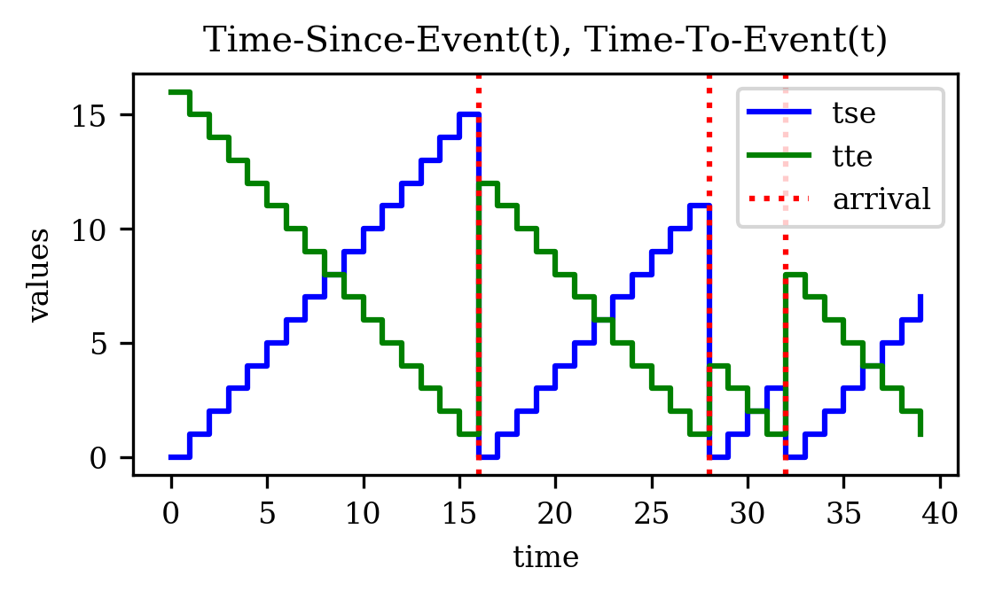
Figure 1: Notation for $\text{tse}(t),\text{tte}(t)$ with three arrivals: The arrival times are at 16, 28 and 32.

The remaining time until next arrival ($Z_{t}$) is a conditional random variable that depends only on $Y_{N(t)+1}$, which is the inter-arrival time of the subsequent arrival. We can thereby define this random variable given the observed information [Equation 5], which is commonly known as a conditional excess random variable [7].

$$Z_{t}=Y_{N(t)+1}-\text{tse}(t)\ |\ Y_{N(t)+1}>\text{tse}(t).$$ (5)

In our approach, we do not model the distribution of $Z_{t}$ directly. Instead, the RNN predict parameters for $Y_{N(t)+1}$ and the losses are computed based on the distribution of $Z_{t}$, which has a distribution induced by $Y_{N(t)+1}$ based on partial information (i.e. $\text{tse}(t)$) . This additional structure helps to simplify the incomplete information problem.

For example, consider $Z=Y-t\ |\ Y>t$. This random variable $Z$ is conditioned on the fact that $Y$ has been observed to exceed $t$ and we are interested in the excess value (i.e. $Y-t$). It is clear that the distribution of $Y$ induces a distribution on $Z$ [Equation 6].

$$P(Z>s)=P(Y-t>s|Y>t)=\frac{P(Y>s+t)}{P(Y>t)}.$$ (6)

III-B Log-Likelihood Computation

There are two cases to properly define the log-likelihood function. When the next arrival time is observed, the likelihood evaluation is $P(Z_{t}\in[\text{tte}(t),\text{tte}(t)+1])$, since inter-arrival times are only discretely observed. However, where the time to next arrival is not observed (i.e. no more subsequent arrivals are observed by end of training), the likelihood evaluation is instead $P(Z_{t}>\text{tte}(t))$, namely the survival function. Therefore at each time $t$, the random variable $Y_{N(t)+1}$ which has distribution parametrized by $\theta_{t}$, induces a distribution on $Z_{t}$. Thus the log-likelihood at each time $t$ can be written as follows [Equation 7].

$$l_{t}(\theta_{t})=\begin{cases}\log P(Z_{t}\in[\text{tte}(t),\text{tte}(t)+1])&\text{if uncensored}\\ \log P(Z_{t}>\text{tte}(t))&\text{otherwise}\end{cases}$$ (7)

In survival analysis terminology, we recall that $Z_{t}$ is the remaining lifetime random variable (i.e. time to death conditioned on current age). For the uncensored case, the likelihood is the death probability and in the right-censored case, it is the survival probability.

We plot distributional estimates at two times to illustrate these cases [Figure 2]. In the uncensored log-likelihood computation, we assume that f3 is the density function of $Z_{3}$, which is the predictive distribution for the remaining time until next arrival at time step 3. Since the next arrival is observed to have occurred at time 6, the remaining time to next arrival is 3, so we evaluate f3 at the value 3. In the censored case, we consider the predictive distribution for remaining time until next arrival at time step 7. We note that the next arrival was not observed by end of training period at time step 10 hence the right tail of $Z_{7}$ (i.e. $\geq 3$) was used to compute the log-likelihood.

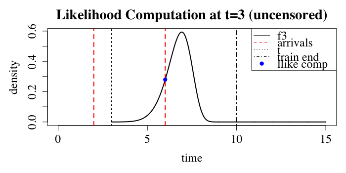
(a) If next arrival is observed then log-likelihood is density

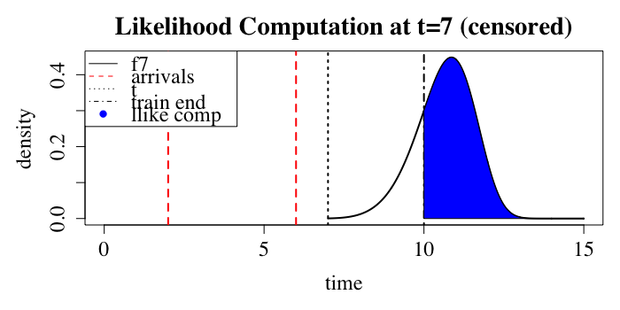
(b) If next arrival is unobserved then log-likelihood is survival.

Figure 2: Log-Likelihood Visualization for Different Censoring Status

It is essential that the class of distributions for $Y_{n}$ is assumed to have differentiable and numerically stable forms for the density and survival functions to exploit the back-propagation algorithm for efficient gradient computation [12]. An example is the Weibull distribution parametrized by scale ($\lambda$) and shape ($k$), which is used in our approach, whose survival function is made up of only exp() and power() functions [Equation 8]. The details of the conditional excess random variables based on Weibull distributions can be found in the Appendix [Section VIII].

$$S(y)=P(Y>y)=e^{-(y/\lambda)^{k}}$$ (8)

III-C An RNN with distributional outputs

A particular RNN structure that had proven to be successful in modeling sequential data is Long Short Term Memory (LSTM) [12], although it can be replaced by other RNN implementations. At each time ($t$), the outputs of the LSTM, which is parametrized by $\Theta$, are passed through an activation function so that they are valid parameters of a distribution function ($\theta_{t}$). Then, the log-likelihood is computed for each time step ($l_{t}$) as defined earlier [Equation 7]. The computational graph is shown [Figure 3], where $h_{t}$ is the internal state of the LSTM and $X_{t}$ are the covariates at each time $t$.

Figure 3: RNN Computational Flow: Outputs ($\theta_{t}$) are generated by an LSTM. Log-likelihoods at each time are computed as log of densities parametrized by $\theta_{t}$, evaluated at $z_{t}$

The loss under such a set-up is the negative of the log-likelihood. Optimal parameters for the LSTM ($\Theta$) are ones that output a series of distributional estimates $\theta_{t}$ that best “explain” the sequence of data observed. In the event of an uncensored arrival time at time $t$, the optimal choice of weights $\theta_{t}$ is one that generates a density that has a peak close to the actual arrival time.

III-D Computing Overall Loss through Conditional Independence

We assume a Bayesian Network similar to a Hidden-Markov model, where random variables at each time $t$ are emitted from a hidden state $h_{t}$ [Figure 4]. Recall that $h_{t}$ represents the internal state of the RNN at each time $t$ [Figure 3], and $Z_{t}$ is the observed time series.

Figure 4: Bayesian Network: Observations are independent conditioned on hidden states

We can therefore factor the joint distribution of $\{Z_{t}\}$, giving the log-likelihood computation for the entire time series as a sum of log-likelihoods at each time, such that we obtain the sum below, for arbitrary events $E_{t}$. Since $E_{t}$ is determined by the censoring status [Equation 7], where $E_{t}=\{[\text{tte}(t),\text{tte}(t)+1]\}$ if uncensored and $E_{t}=\{>\text{tte}(t)\}$ otherwise, we can decompose the overall log-likelihood as a sum [Equation 9].

$$P(\{Z_{t}\in E_{t}\}_{t=1}^{\tau}|\ \{h_{t}\}_{t=1}^{\tau}) =\prod_{t=1}^{\tau}P(Z_{t}\in E_{t}|\ h_{t})$$ (9)

$$l(\{\theta_{t}\}) =\sum_{t}l_{t}(\theta_{t})$$

Assuming that the LSTM/RNN is parametrized by $\Theta$, we note that there exists a function $g$ that recursively maps $X_{t}$ to $(\theta_{t},h_{t})$ that depends only on $\Theta$ [Equation 10]. By substituting $h_{t-1}$, we can write $l_{t}(\theta_{t})=l_{t}(g_{t}(\Theta))$ where $g_{t}$ depends only on $\Theta,g,\{X_{l}\}_{l\leq t}$. Then since the overall log-likelihood is a sum of $l_{t}(\theta_{t})$, it can be written as a function of only the RNN parameters ($\Theta$) and observed data. The structure of the RNN and the back-propagation algorithm allows us to compute gradients of any order efficiently and therefore find the $\hat{\Theta}$, the minimizer of the overall observed loss [12].

$$(\theta_{t},h_{t})=g(h_{t-1},X_{t}\ |\ \Theta)$$ (10)

III-E Activation Functions for Distributional Parameters

The neural net outputs must be transformed such that they are parameters of a distribution. In our case, we used a Weibull distribution, which is parametrized by shape and scale parameters, both of which are positive values. We initialized the RNN output for scale at the maximum-likelihood estimate (MLE) for the scale parameter of a Weibull distribution whose shape parameter is 1 as this was found to be useful in preventing likelihood-evaluation errors [21]. We also chose a maximum shape parameter (set at 10) and pass the RNN output for shape through a sigmoid function, which is rescaled and shifted such that $\sigma^{*}:\mathbb{R}\rightarrow(0,10)$ and $\sigma^{*}(0)=1$. For the scale parameter, an exponential function is used, which is rescaled such that it maps 0 to the average inter-arrival-time.

III-F Extension to Multi-Variate Waiting Times

To model multivariate arrivals, we assume there are $p$ different arrival processes of interest. For the $i$-th waiting time of interest, we define $W_{i,n}$ to be the time of the $n$-th arrival of this type and $N_{i}(t),Y_{i,n}$ be likewise defined. We also need to define $\text{tse}(i,t),\text{tte}(i,t)$ to be that for the $i$-th type as well. Similarly define its associated conditional excess random variable [Equation 11].

$$Z_{i,t}=Y_{i,N_{i}(t)+1}-\text{tse}(i,t)\ |\ Y_{i,N_{i}(t)+1}>\text{tse}(i,t)$$ (11)

In the earlier framework [Figure 4], we can let $Z_{t}=[Z_{1,t},\ldots,Z_{p,t}]$ and let the RNN output $\theta_{t}=[\theta_{1,t},\ldots,\theta_{p,t}]$.

Then we write the log-likelihoods for each event type where $l_{i,t}(\theta_{i,t})=\log P(Z_{i,t}=\text{tte}(i,t))$ or $l_{i,t}(\theta_{i,t})=\log P(Z_{i,t}>\text{tte}(i,t))$, recalling that the former is for the case where the next arrival is observed while the latter is for the case where the no arrivals are observed until the end of training.

The earlier Bayesian Network structure [Figure 4] requires minimal modifications as we merely require that the emissions are conditionally independent given $h_{t}$. This then allows us to compute the log-likelihood at each time as a sum, $l_{t}(\theta_{t})=\sum_{i}l_{i,t}(\theta_{i,t})$. Since the LSTM network is still parameterized by $\Theta$, the remaining operations are exactly the same as earlier. In this way, temporal dependence as well as dependence between the $p$ arrival processes can be modeled by the RNN, whose weights $\Theta$ will then be optimized by training data. This allows us to model other outputs as well by appending $[K_{1,t},\ldots,K_{p,t}]$ to $Z_{t}$ where $K_{j,t}$ is some other variable of interest for process $j$ at time $t$.

III-G Masking of Non-Inter-Arrival-Times

In multi-variate purchase arrival times, we found that masking sequences observed before the first arrival of each product is useful in preventing numerical errors encountered in stochastic gradient descent. As such, log-likelihoods computed for time steps before the earliest arrival are masked. This ensures that RNN parameters are not updated due to losses incurred during these times.

III-H Predicting Time to Next Arrival

Predictions are simple to compute since at each time $t$, we can use the estimated parameter $\theta_{t}$ to compute the expectation of any function of $Z_{t}$, assuming that $Z_{t}$ is distributed according to $\theta_{t}$. Since we are concerned with the next arrival time after the end of training period (time $\tau$), we can compute many different values of interest.

For example, if we want to find the predicted probability that the next arrival will occur within $\gamma$ time after end of training, we can compute $P(Z_{\tau}\leq\gamma)$. We can also compute a deferred arrival probability, which is the probability that the next arrival will occur within an interval between $\gamma_{1}$ and $\gamma_{1}+\gamma_{2}$ time after end of training given that we know it will not occur within $\gamma_{1}$ time after the end of training. This can be found by computing $P(Z_{\tau}\in[\gamma_{1},\gamma_{1}+\gamma_{2}]\ |\ Z_{\tau}>\gamma_{1})$. The quantities of interest may not necessarily be limited to probabilities (e.g. mean, quantiles of the predictive distribution) and can be extended to generate other analytics for revenue analysis or forecasting that depends on the subsequent purchase time.

IV Experimental Results

We ran experiments to show the efficacy of the proposed model. Since our model provides distributional estimates for time to next event, we can evaluate its performance in a binary classification framework as well as in a regression context. This is explored by running experiments on two open datasets. The first is store purchases so there are multiple arrivals but with no covariates. The second is failure time prediction with many covariates. Finally, we apply the model to a real dataset of retail purchases in order to compare real-world performances of the considered models. We were unable to find open data for multivariate arrival times with a large number of arrival types but the publicly available code can be easily extended to run on such data.

IV-A Performance Evaluation

Binary classification performance is evaluated using the Receiver Operating Characteristics Area Under Curve (ROC-AUC), which is equivalent to the Concordance Index (C-Index) commonly used in survival analysis [11]. Point prediction performance is evaluated using specified distance metrics.

IV-B Recurrent Neural Net Structure

For all experiments in this section, a simple structure for our neural net is chosen where there are only three stacked layers, with two LSTM layers of size $W$ followed by a densely connected layer of size $2p$, where $p$ is the number of arrival processes. The densely connected layer transforms the LSTM outputs to a vector of length $2p$. We chose a Weibull distribution as the family of distributions for our inter-arrival times, which has two parameters, namely the scale and shape. In MAT-RNN, the outputs are then passed through an activation layer [Section III-E]. For squared-loss RNNs, the activation is passed through a softplus layer since time to arrivals are non-negative. A masking layer is applied prior to the other layers on time indices prior to the initialization of the time series so that losses incurred during those time steps do not affect optimization.

Figure 5: Recurrent Network Setup for a $p$-variate Arrival Process with $W$-long Hidden State

This structure is the same for other neural network based models used for benchmark comparison. The networks are trained with Adam [16] and non-default training parameters are specified where possible. Gradients are component-wise clipped at $5$ to prevent numerical issues. Implementation was done using Keras [4] as our TensorFlow [5] wrapper. Evaluation metrics and ensemble predictors are implemented using scikit-learn [24]. Implementations and comparisons on open datasets will be published on a publicly-accessible repository .

IV-C Comparisons on Open Datasets

We show the flexibility of the proposed MAT-RNN model with two open dataset benchmarks. These two problems are often tackled with different models since the prediction problem is different. The proposed MAT-RNN model however, can be adapted to solve these problems since they can be modeled by a distributional approach to inter-arrival times.

The first example is the CDNOW dataset [Section IV-C1]. We consider a binary classification problem where we predict if purchases are made during a testing period. Predictions from MAT-RNN can be computed as the probability that the inter-arrival time occurs before the end of the testing period. Data available is limited to only the transaction history (i.e. purchase date, purchase quantity, customer id, etc) without other covariate data. This type of data is particularly suited to the simple Pareto/NBD type models discussed earlier. We show that MAT-RNN out-performs on a dataset even with no covariates.

The second example is based on the CMAPSS dataset [Section IV-C2] where we predict the remaining useful lifetime, or the time to failure. Predictions from MAT-RNN can be computed as the mode, mean or some other function of the inter-arrival time distribution. The training data is an uncensored time series where sensor readings and operational settings are collected until the engine fails. A customized loss function was used to evaluate models in the PHM08 competition [26], which we will include for our evaluation. Since the training data is fully observed, we would expect the RNN model to perform well.

IV-C1 Binary Classification Comparison on CDNOW

Purchase transactions are available from the CDNOW dataset [10] where number of customer purchases are recorded. Only transaction dates, purchase counts and transaction value are available as covariates. Our model is trained on weekly purchases and hidden layers are 1-long (i.e. $W=1$ [Section IV-B]). Binary classification performance is compared to the Pareto/NBD model, which is a classical demand forecasting model [29] using the lifetimes package [3]. This dataset is often used as an example where Pareto/NBD type models do well since there’s limited covariate data available and there’s only a single event type.

With $W=1$, there are only $32$ trainable parameters in the MAT-RNN model. The training period is set at 1.5 years, from 1997-01-01 to 1998-05-31. Predictions are made for customer purchases within a month of the end of training (i.e. before 1998-06-30). We see that MAT-RNN achieves an ROC-AUC of 0.84 which is better compared to 0.80 that is obtained using the Pareto/NBD estimate for the “alive” probability [Figure 6]. Results from WTTE-RNN are similar and yields almost the same ROC-AUC curve. This is likely due to the mostly memoryless nature of these customer purchases. It can be seen that this approach of integrating a survival-based maximum log-likelihood method with a RNN can yield improved prediction accuracy even with a small number of weights and on a small dataset.

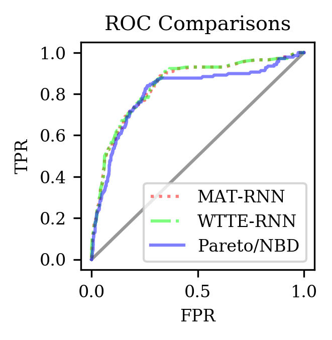
Figure 6: ROC Curves for CDNOW predictions

IV-C2 Point Estimate Comparison on CMAPSS

The CMAPSS dataset [27], is a high dimensional dataset on engine performance with 26 sensor measurements and operational settings. In the training model, the engines are run until failure. In the testing model, data is recorded until a time prior to failure. The goal is to predict the remaining useful life (RUL) for these engines. We used the first set of engine simulations in the dataset (train_FD001.txt) which has 100 uncensored time series of engines that were run until failure. The maximum cycles run before failure was found to be at 363. Time series for each engine was segmented into sliding windows of window length 78, resulting in 323 windowed time series each of length 78. For the testing dataset, RNN is run on time series 78 cycles before end of observation.

A custom loss function was defined for the PHM08 conference competition that was based on this dataset, where over-estimation is more heavily penalized [26]. The loss function is defined as follows, where $d$ is the predicted RUL subtracted by the true RUL [Equation 12].

$$\text{loss}(d)=\begin{cases}e^{-d/13}-1&d<0\\ e^{d/10}-1&d>0\\ \end{cases}.$$ (12)

We compare the performances of the RNN models since they are able to make point predictions fro RUL. The SQ-LOSS model was used with a softplus activation layer scaled by average failure time and the weights are fitted on squared loss. The RNN models were trained with $W=64$ [Section IV-B], where there are 2 hidden layers each of $W$-long. A variety of training iterations and learning rates were used, and a grid search was performed over all combinations. Performance is evaluated on the test set based on the root mean squared loss metric (rMSE) as well as the mean custom loss metric (MCL) [Equation 12]. Testing set losses are presented in a table [Table I]. We find that MAT-RNN is generally easier to train, achieving the smallest losses under almost all hyper-parameters other than a slow learning rate and small training iteration.

TABLE I: Comparison on RNN-based Methods for CMAPSS

lr	iters	loss	MAT-RNN	WTTE-RNN	SQ-LOSS
1e-3	1e2	MCL	41.79	275.73	262.39
		rMSE	32.82	41.05	42.50
	1e4	MCL	41.79	275.73	262.39
		rMSE	32.82	41.05	42.50
1e-4	1e2	MCL	45.84	355.48	446.88
		rMSE	33.16	42.10	47.53
	1e4	MCL	41.79	275.73	262.39
		rMSE	32.82	41.05	42.50
1e-5	1e2	MCL	1926.13	386.16	10041.36
		rMSE	53.16	42.04	60.22
	1e4	MCL	29.34	36.84	262.39
		rMSE	28.85	31.49	42.50

We visualize the predictions of the best performing model, achieved by MAT-RNN with $\text{iters}=1e4,\text{lr}=1e-5$ [Figure 7]. As expected, we find that the predicted density of the remaining lifetime to be highest at the true RUL. Taking point estimate as the model of the predicted density, we can then plot predicted RUL against true RUL, which indicates that we have a good predictive accuracy.

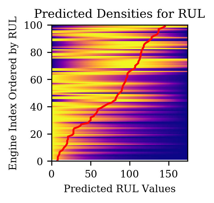
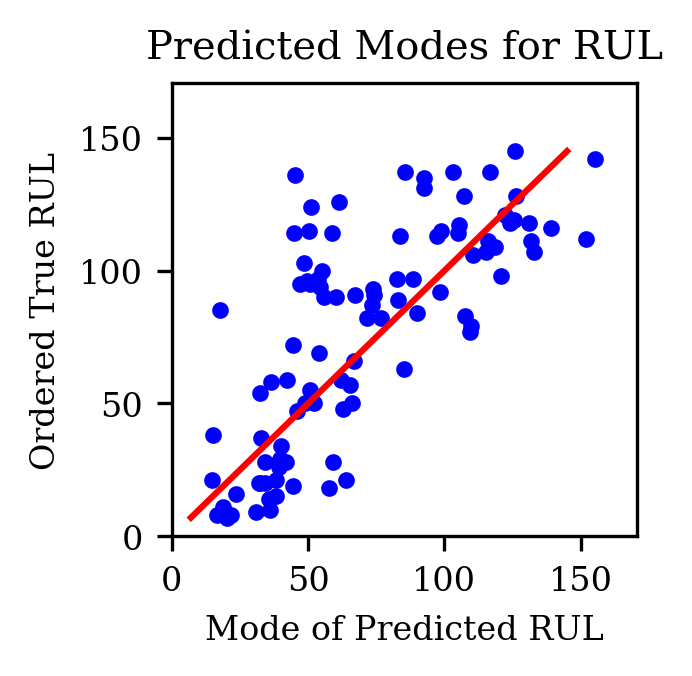
Figure 7: Predicted RUL Density and Mode on C-MAPSS and True RUL (in red) for MAT-RNN with $1e4$ iterations and $1e-5$ learning rate.

IV-D Demand Forecasts for a Large Retailer

We investigate the predictive performance for purchases of of a few baskets of goods sold by a large retailer. The time resolution of our dataset is on a weekly level. Training data is available over roughly 1.5 years, which gives us 78 weeks of training data from 2014-01-01 to 2015-06-30. Performance of our MAT-RNN model is measured on the binary classification problem of predicting whether a customer purchases the product within 4 weeks after the end of training period from 2015-06-30 to 2015-07-31.

IV-D1 Benchmark Models

Even though our model can predict many different quantities of interest [Section III-H], we chose to compare the predictive performance to a few benchmark models in terms of whether an event will arrive within $\gamma$ time after the end of the training period. These models are namely the Squared-Loss RNN (SQ-RNN) and a Random Forest Predictor (RNG-F), which are state-of-the-art models in personalized demand forecasting [20] and forecasting event arrival times [1]. Models are trained on all customers who bought an item in the basket during the training period and performance is evaluated on this group of customers during the testing period.

• RNG-F is trained by splitting the training period into two periods. Covariates at the end of the first period are fed into the model, which is trained to predict whether subjects purchase in the second period of length $\gamma$. A different RNG-F model is trained for each product, but is fed covariate datasets for all products.

• SQ-LOSS is trained by setting the loss function as the squared difference between the predicted time-to-arrival and the actual time-to-arrival. An activation function of softplus is applied. Predictions of SQ-LOSS are then compared to the testing period length of $\gamma$. If by the end of the training period, SQ-LOSS predicts the next time-to-arrival as $s$, then the prediction metric is $\gamma-s$. For time periods where no actual time-to-arrival was observed (i.e. no further purchases were observed by end of training), loss is set to 0.

IV-D2 Covariates

For each customer, at each time period, we compute the Recency, Frequency and Monetary (RFM) metrics which are commonly used in demand modeling [20] at three different levels: namely for all products, in-basket products and each individual product. Recency is the time since last purchase, frequency is the number of repeat purchases and monetary is the amount of money spent on all purchases to date. Included in the covariates are time-since-event ($\text{tse}(t)$) and indicators for whether a first purchase has occurred ($\text{pch}(t)$). We also compute the time-to-event ($\text{tse}(t)$) as well as the censoring status of the next arrival ($\text{unc}(t)$), which are only passed to the loss function.

On a per-product level, the types of covariates are limited to only RFM metrics (3 covariates) and transformations of purchase history (2 series). RFM metrics on the category and overall purchase history levels are available as well, but these account for an additional 6 covariates that are shared across the various purchase arrival processes. The total number of covariates for each product is thus 11, of which 6 are shared with other products.

IV-D3 Data Summaries for Product Baskets

We selected 5 baskets of popular replenishable products. These are selected from products ranked by a score, where $N_{\text{unique}}$ is the number of unique customers and $X$ is the average purchases per customer.

$$\text{score}=X*\log N_{\text{unique}}$$ (13)

The selected baskets are bars, deli, floss, pads, soda. Their data summaries are presented [Table II], where $\mu_{\text{overall}}$ is the average in-basket purchase counts, $\mu_{\text{per-sku}}$ is the mean over the per-product average purchase counts and $p_{\text{others}}$ is the mean over the per-product proportion of buyers who bought another product in-basket. Also note that $p_{\text{trial}}$ is the mean over the per-product proportion of trial customers (i.e. those who have made only a single purchase).

TABLE II: Data Summary of Product Baskets

		customers
basket	SKUs	(x1000)	$\mu_{\text{overall}}$	$\mu_{\text{per-sku}}$	$p_{\text{others}}$	$p_{\text{trial}}$
bars	6	44	4.78	0.79	0.71	0.43
deli	12	79	3.58	0.29	0.55	0.62
floss	11	200	2.58	0.23	0.40	0.64
pads	7	317	2.26	0.32	0.28	0.66
soda	8	341	2.97	0.37	0.45	0.63

We note that pads has the highest proportion of trial customers along with the smallest proportion of customers who bought another item in the basket. On the other hand, we find that $\mu_{\text{per-sku}}$ is roughly median in the baskets considered. This is similar for floss as well. For these categories, it would be reasonable to expect product purchases are strongly dependent. A good joint-prediction model should separate trial purchasers from repeat purchasers who decided to stick to one product after trying another.

IV-D4 Performance of Joint Predictions

Performance is measured based on the ROC-AUC metric where each of the models (i.e. RNG-F, SQ-LOSS, MAT-RNN) predict whether customers who made in-basket purchases will make another in-basket purchase in a 4 week period after the end of a training period of 78 weeks. Framing this as a binary prediction problem allows us to compare these state-of-the-art models. The RNN-based models share the same network specifications with $W=36$ [Section IV-B] and predict arrival times jointly over different products for each customer. These models are run for 100 iterations with a learning rate set to $1e-3$. The RNG-F model is trained with 100 trees with covariates at week 74 and purchases between week 74 and 78 but predicts purchases for only one product at a time using default parameters in scikit-learn. As such, a separate RNG-F model is trained for each product. We note that RNG-F model is favored since the training metric is directly related to the testing metric, whereas the RNN-based models train and predict based on arrival times.

TABLE III: ROC-AUC for Products in Category. Empirical quantiles are taken over per-product ROC-AUCs in each category.

	Customers			# Improved	ROC-AUC Quantiles					ROC-AUC
Category	(x1000)	Products	Model	over RNG-F	Min	Q25	Q50	Q75	Max	Average
bars	44	6	RNG-F	-	0.7696	0.7986	0.8428	0.8648	0.8710	0.8304
			SQ-LOSS	0	0.6608	0.7165	0.7228	0.7406	0.7550	0.7204
			MAT-RNN	2	0.7588	0.7762	0.8174	0.8537	0.8783	0.8167
deli	79	12	RNG-F	-	0.7452	0.7995	0.8389	0.9004	0.9220	0.8468
			SQ-LOSS	4	0.7763	0.8047	0.8248	0.8458	0.8810	0.8259
			MAT-RNN	8	0.8686	0.8823	0.8911	0.9021	0.9131	0.8919
floss	200	11	RNG-F	-	0.5537	0.6066	0.6199	0.6517	0.7683	0.6408
			SQ-LOSS	10	0.7298	0.7809	0.8089	0.8366	0.8739	0.8055
			MAT-RNN	11	0.8680	0.9016	0.9317	0.9421	0.9640	0.9214
pads	317	7	RNG-F	-	0.5851	0.6148	0.6358	0.6411	0.8234	0.6509
			SQ-LOSS	4	0.5650	0.6149	0.6392	0.6941	0.7154	0.6482
			MAT-RNN	7	0.8544	0.9160	0.9459	0.9511	0.9621	0.9281
soda	341	8	RNG-F	-	0.6959	0.7372	0.7663	0.7903	0.8300	0.7641
			SQ-LOSS	1	0.6844	0.7221	0.7259	0.7320	0.7612	0.7258
			MAT-RNN	8	0.8605	0.8669	0.8795	0.8854	0.8909	0.8768

We are interested in the performance of each model for every product in the basket so there are multiple ROC-AUC metrics. The results are presented in terms of summary statistics for ROC-AUCs for each item in the basket [Table III]. In our testing, we found that the MAT-RNN model almost always dominates in the ROC-AUC metric for every category other than bars and deli, which has the smallest number of customers. Even so, MAT-RNN still performs the best in terms of average ROC-AUC among products in each category [Table III] other than bars.

The number of products for which ROC-AUC has improved over RNG-F is substantial for MAT-RNN. Excluding bars where only 2 out of 6 products saw improved performance, other categories saw ROC-AUC improvements in more than 60% of the products in-category, with soda and pads showing improvements in all products. The ability to model sequential data and sequential dependence separates MAT-RNN model from RNG-F. Even though RNG-F is trained on the evaluation metric, we find that MAT-RNN almost always performs better in this binary classification task.

Also notable is that the performance difference of MAT-RNN over SQ-LOSS and RNG-F is greatest for the pads category. This is likely due to the large amount of missing data since customers are least likely to buy other products [Table II]. We also find that SQ-LOSS performs poorly compared to MAT-RNN [Table III], even though these models have the same recurrent structure and are fed the same sequential data. One possible explanation is that the lack of ground truth data has a significant impact on the ability of SQ-LOSS to learn. In cases where event arrivals are sparse or where inter-purchase periods are long, the censored nature of the data gives no ground truth to train SQ-LOSS on. Therefore, even though the recurrent structure makes it possible to model sequential dependence, the structure that MAT-RNN imposes on the problem makes it much easier to make predictions with censored observations.

We should note that RNG-F out-performs MAT-RNN for 4 out of 12 deli products and 4 out of 6 bars products. A possible reason is that these categories have a smaller sample size. One limitation of the RNN models is that regularization options are more limited compared to ensemble methods used in RNG-F. Based on the results, it appears that MAT-RNN performs better for more customers [Table III].

IV-D5 Joint Predictions and Individual Predictions

It is clear that joint predictions enjoy some advantages over individual predictions. As stated earlier, we expect correlations in product purchases to be modeled better through joint modeling. If network structure is the same, then the amount of time required to train a separate model for each product scales linearly with the number of products. The number of parameters in a collection of individual models is also significantly larger than that of a joint model.

We study the advantages of training a joint MAT-RNN model over a collection of individual ones by comparing ROC-AUC performance in the soda basket. The per-product individual models are given the same covariates but trained only on the purchase arrivals of that particular product. The network structure is the same with $W=36$, but the final densely connected layer outputs only a vector of size 2, since distributional parameters for one product is required. However, since the collection of single models have different weights for their RNNs, they have approximately 8 times the number of parameters found in the joint model. We observe a consistent advantage of a joint model over the individually trained single models, with improvements ranging from 0.0029 to 0.1098 [Table IV]. It is clear that potential improvements in model performance can be observed by modeling purchase arrivals jointly, even with much fewer parameters in the joint model.

TABLE IV: Comparison of ROC-AUC performance on soda for single and joint MAT-RNN models

sku	single	joint	diff
1	0.8868	0.8897	+0.0029
2	0.8073	0.8686	+0.0614
3	0.8331	0.8605	+0.0274
4	0.8501	0.8761	+0.0260
5	0.8445	0.8829	+0.0384
6	0.8193	0.8615	+0.0422
7	0.8640	0.8909	+0.0269
8	0.7742	0.8840	+0.1098

V Conclusion

We described a method to incorporate a survival analysis approach with recurrent neural nets (RNN) to forecast joint arrival times till next purchase for each individual customer over multiple products. This was achieved by transforming the arrival time problem into a likelihood-maximization one with loose distributional assumptions regarding inter-arrival times. Our experiments show that this leads to significant improvement over current state-of-the-art methods is possible. This is the result of being able to model purchases jointly as well as combining a parametric approach to modeling partially observed information with recent advances in neural networks.

VI Future Work

Future work includes modeling more features, as the structure allows for the observed processes to be independent given the parameter generation process. An extra feature to model is first-arrival times, which can help predict whether a customer might make their first purchase in response to marketing campaigns. However, to model this effectively, we require a model-based solution to address the sparsity of observations of first-arrival times.

VI-A Scaling to Inventory-Wide Predictions

Including thousands of products is infeasible in the current implementation. It would be useful to extend the model to make joint inventory-wide predictions for purchase arrival times. Inventory-wide predictions also brings about other technical problems such as memory usage and ETL (data extraction, transformation, loading). The computation of time-since-event and time-to-event as well as other features to be used in log-likelihood computation [Section III-B] is also problematic in that it transforms a sparse dataset (i.e. transactional information) into a dense dataset (i.e. temporal data). An inventory-wide extension needs to address these issues by either implementing an efficient method to compute these matrices or avoid the problem through a variant of MAT-RNN. Nonetheless, we believe that the current implementation can suffice for the purposes of targeted advertising where we are only interested in predicting demand and pushing sales for a few product lines.

VII Acknowledgments

We would like to thank Kanchana Padmanabhan and Erin Wilder at Rubikloud Technologies Inc for their expertise in editing this paper as well as the Data Science and Engineering team for their technical support. This would also not have been possible without the supervision and advice of Professor Nancy Reid and Professor Andrei Badescu at the University of Toronto. Lastly, we’d like to thank the NSERC (Natural Sciences and Engineering Research Council) Engage and Mitacs Accelerate programs for funding this project.

VIII Appendix: Weibull Likelihoods

A random variable $Y\sim\texttt{Weibull}(\textbf{scale}=\lambda,\textbf{shape}=k)$ has simple densities and cumulative distribution functions, since the survival function $(S(x))$ has a simple form:

$$S(y) =P(Y>y)$$ (14)

$$=e^{-(y/\lambda)^{k}}.$$

$$f(y) =(k/\lambda)(y/\lambda)^{k-1}e^{-(y/\lambda)^{k}}$$

$$=(k/\lambda)(y/\lambda)^{k-1}S(y).$$

The conditional excess random variable, given that it exceeds $s$, is $W=Y-s|Y>s$. Recall the definition of conditional probability in terms of some continuous random variable $X_{1},X_{2}$, for any measurable set $A_{1},A_{2}$, given $P(X_{2}\in A_{2})>0$:

$$P(X_{1}\in A_{1}|X_{2}\in A_{2})=\frac{P(X_{1}\in A_{1},X_{2}\in A_{2})}{P(X_{2}\in A_{2})}.$$ (15)

We can therefore derive the conditional excess survival function:

$$S_{W}(t) =P(W>t)$$ (16)

$$=P(Y>s+t|Y>s)$$

$$=S(s+t)/S(s)$$

$$=\exp\left\{-((s+t)/\lambda)^{k}+(s/\lambda)^{k}\right\}.$$

Also, we can find the conditional excess density function:

$$f_{W}(t) =f(s+t)/S(s)$$ (17)

$$=(k/\lambda)((s+t)/\lambda)^{k-1}S(s+t)/S(s)$$

$$=(k/\lambda)((s+t)/\lambda)^{k-1}S_{W}(t).$$

References

- [1] Edward Choi, Mohammad Taha Bahadori, Andy Schuetz, Walter F. Stewart, and Jimeng Sun. Doctor ai: Predicting clinical events via recurrent neural networks. arXiv, 1511.05942, 2015.
- [2] D. R. Cox and D. Oakes. Analysis of Survival Data. Chapman and Hall, United Kingdom, 1984.
- [3] Cameron Davidson-Pilon. github.com/CamDavidsonPilon/lifetimes, 2001.
- [4] François Chollet et al.
- [5] Martin Abadi et al. Tensorflow: Large-scale machine learning on heterogeneous systems. https://www.tensorflow.org/, 2015.
- [6] Peter S. Fader, Bruce G. S. Hardie, and Ka Lok Lee. Counting your customers the easy way: An alternative to the pareto/nbd model. Marketing Science, 24(2):275–84, 2005.
- [7] Maxim Finkelstein. Failure Rate Modelling for Reliability and Risk. Springer, London, 2008.
- [8] Valentin Flunkert, David Salinas, and Jan Gasthaus. Deepar: Probabilistic forecasting with autoregressive recurrent networks. arXiv, 1704.04110, 2017.
- [9] Alex Graves, Abdel-Rahman Mohamed, and Geoffrey Hinton. Speech recognition with deep recurrent neural networks. Proceedings of IEEE International Conference on Acoustics and Speech and Signal Processing, 1:6645–49, 2013.
- [10] Bruce Hardie. www.brucehardie.com/datasets/CDNOW_master.zip, 2001.
- [11] Frank E Harrell, Kerry L Lee, Robert M Califf, David B Pryor, and Robert A Rosati. Regression modeling strategies for improved prognostic prediction. Statistics in Medicine, 3(2):143–152, 1984.
- [12] Sepp Hochreiter and Jurgen Schmidhuber. Long short-term memory. Neural Computation, 9:1735–80, 1997.
- [13] Direct Marketing Association (U.S.) Global Insight Inc. The Power of Direct Marketing: ROI, Sales, Expenditures, and Employment in the U.S. DMA, New York and NY, 13 edition, 2009.
- [14] Rashmi Joshi and Colin Reeves. Beyond the cox model: artificial neural networks for survival analysis part ii. Proceedings of the eighteenth inter-national conference on systems engineering, 1:179–84, 2006.
- [15] Jared Katzman, Uri Shaham, Jonathan Bates, Alexander Cloninger, Tingting Jiang, and Yuval Kluger. Deepsurv: Personalized treatment recommender system using a cox proportional hazards deep neural network. Proceedings of International Conference of Machine Learning Computational Biology Workshop, 2016.
- [16] Diederik P. Kingma and Jimmy Ba. Adam: A method for stochastic optimization. Proceedings of The 3rd International Conference for Learning Representations, -, 2015.
- [17] John P. Klein and Melvin L. Moeschberger. Survival analysis: Techniques for censored and truncated data. Springer, 2003.
- [18] Bart Lariviere and Dirk Van den Poel. Investigating the role of product features in preventing customer churn and by using survival analysis and choice modeling: The case of financial services. Expert Systems With Applications, 27(2):277–285, 2004.
- [19] Linxia Liao and Hyung il Ahn. Combining deep learning and survival analysis for asset health management. The International Journal of Prognostics and Health Management, 7(020):7, 2016.
- [20] Gordon Linoff and Michael Berry. Data Mining Techniques: For Marketing and Sales and and Customer Relationship Management. Wiley, New York and NY, 2004.
- [21] Egil Martinsson. Wtte-rnn : Weibull time to event recurrent neural network. Master’s thesis, Chalmers University Of Technology, 2016.
- [22] McKinsey Practice Publications. Perspectives on retail and consumer goods. 2016.
- [23] Rupert G. Miller. Survival analysis. John Wiley & Sons, 1997.
- [24] Fabian Pedregosa, Gael Varoquaux, Alexandre Gramfort, Vincent Michel, Bertrand Thirion, Olivier Grisel, Mathieu Blondel, Peter Prettenhofer, Ron Weiss, Vincent Dubourg, Jake Vanderplas, Alexandre Passos, David Cournapeau, Matthieu Brucher, Matthieu Perrot, and Edouard Duchesnay. Scikit-learn: Machine learning in python. Journal of Machine Learning Research, 12:2825–30, 2011.
- [25] David M. W. Powers. Evaluation: From precision, recall and f-measure to roc, informedness, markedness & correlation. Journal of Machine Learning Technologies, 2(1):37–63, 2011.
- [26] Emmanuel Ramasso and Abhinav Saxena. Performance benchmarking and analysis of prognostic methods for cmapss datasets. International Journal of Prognostics and Health Management, 5(2):15, 2014.
- [27] Abhinav Saxena, Kai Goebel, and Don Simon. Damage propagation modeling for aircraft engine run-to-failure simulation. International Conference on Prognostics and Health Management, page 1–9, 2008.
- [28] Juergen Schmidhuber. Deep learning in neural networks: An overview. Neural Networks, 61:85–117, 2015.
- [29] David C. Schmittlein, Donald G. Morrison, and Richard Colombo. Counting your customers: Who are they and what will they do next? Management Science, 33:1–24, January 1987.
- [30] Rafet Sifa, Fabian Hadiji, Julian Runge, Anders Drachen, Kristian Kersting, and Christian Bauckhage. Predicting purchase decisions in mobile free-to-play games. Proc. of AAAI AIIDE, (78), 2015.
- [31] David C Yen, Shin-Yuan Hung, and Hsiu-Yu Wang. Applying data mining to telecom churn management. Expert Systems with Applications, 31.3:515–24, 2006.