Fermion-parity switches of the ground state of Majorana billiards

Abstract

Majorana billiards are finitely sized, arbitrarily shaped superconducting islands that host Majorana bound states. We study the fermion-parity switches of the ground state of Majorana billiards. In particular, we study the density and statistics of these fermion-parity switches as a function of applied magnetic field and chemical potential. We derive formulae that specify how the average density of fermion-parity switches depends on the geometrical shape the billiard. Moreover, we show how oscillations around this average value is determined by the classical periodic orbits of the billiard. Finally, we find that the statistics of the spacings of these fermion-parity switches are universal and are described by a random matrix ensemble, the choice of which depends on the antiunitary symmetries of the system in its normal state. We thus demonstrate that “one can hear (information about) the shape of a Majorana billiard” by investigating its “fermion-parity switch spectrum”.

I Introduction

Eigenvalue spectra of finite quantum systems are related to their shape in the short wavelength limit REF:Book:Weyl68 ; REF:Book:Baltes76 . The celebrated Weyl expansion relates the smooth part of the density of states to the volume, boundary area, curvature as well as the Euler characteristics of the shape of the system REF:Balian70 ; REF:Book:Baltes76 ; REF:Book:Brack03 . The remaining part, namely the density of states fluctuations, sensitively depends on the set of periodic orbits of the corresponding classical dynamics as well as the type of scattering featured in the system REF:Balian72 ; REF:Berry85 ; REF:Book:Gutzwiller90 ; REF:Book:Mehta04 ; REF:Wurm09 . Moreover, if all unitary symmetries are completely broken, the level-spacing distribution becomes universal and reflects the presence (or absence) of antiunitary symmetries REF:Wigner55 ; REF:Dyson62 ; REF:Dyson62b ; REF:Dyson63 ; REF:Bohigas84 ; REF:Book:Mehta04 .

The ground state of conventional superconductors have even number of fermions, reflecting their completely paired nature (even fermion-parity). However, under certain conditions, the energy level of a state with an odd number of fermions (odd fermion-parity) can cross the the energy level of the state with even fermion-parity to become the new ground state. This crossing, dubbed fermion-parity crossing (FPX), is protected since perturbations that mix different fermion-parity states are prohibited. While well known within the context of impurity states in superconductors REF:Balatsky06 ; REF:Mi14 , these crossings can be viewed as topological phase transitions REF:Fu09 ; REF:Ryu10 ; REF:Stanescu11 ; REF:Lee12 ; REF:Beenakker13b ; REF:Rieder13 ; REF:Chang13 ; REF:Sau13b ; REF:Badiane13 ; REF:Chevallier2013 ; REF:Lee14 ; REF:Hedge15 . The modes that form at the degeneracy point are the well known Majorana zero modes featuring non-Abelian statistics REF:Kitaev01 ; REF:Hasan10 ; REF:Qi11 ; REF:Alicea12 ; REF:Book:Bernevig13 ; REF:Elliott15 , which have attracted recent attention as the candidate system for realization of topological quantum computers.

Currently there are experimental signatures of zero-bias conductance peaks, suggestive of edge-bound zero-bias states REF:Mourik12 ; REF:Nadj-Perge14 ; REF:Fornieri19 ; REF:Vaitiekenas18 . However, conclusive experimental demonstration of the Majorana bound states has been elusive so far as these observed peaks could have non-topological origins such as Andreev bound states REF:Lee14 ; REF:Hsieh2012 ; REF:Prada12 ; REF:Chevallier2013 ; REF:Silva2016 ; REF:Liu2017 ; REF:Nichele2017 ; REF:Zuo2017 ; REF:Tang2018 ; REF:Moore2018a ; REF:Hell2018 ; REF:Liu18 ; REF:Vuik2018 ; REF:Moore2018b ; REF:Reeg2018 ; REF:Kayyalha2019 ; REF:Chen2019 ; REF:Woods2019 ; REF:Cao2019 , Kondo effect, weak antilocalization, and disorder REF:Motrunich2001 ; REF:Brouwer2011a ; REF:Brouwer2011b ; REF:Pikulin12 ; REF:Popinciuc2012 ; REF:Bagrets12 ; REF:Liu12 ; REF:Neven2013 ; REF:Churchill13 ; REF:Sau2013a ; REF:Pan2019 . Hence new methods of distinguishing Majorana zero modes from other sources as well as new ways of understanding these nanowires has become desirable. The presence of FPX sequences has been regarded as the smoking gun signature of Majorana states in ballistic 1D wires REF:DasSarma12 ; REF:Rodriguez-Mota19 . The universal statistics of these FPXs were first studied by Beenakker et al REF:Beenakker13b . Recent measurements on proximity coupled nanowires, expected to feature topological superconductivity, found sequences of FPXs as a function of magnetic field as well as gate voltage REF:Chen2019 ; REF:Woods2019 .

In this work, we study the FPXs in finite sized topological superconducting systems through the lens of (i) spectral geometry, (ii) semiclassical physics and (iii) random matrix theory. We call these finite superconducting systems that feature FPXs Majorana billiards (MBs) REF:Footnote:MBRealizations . These FPXs in MBs occur as an external parameter of the system, such as the chemical potential $\mu$ or the Zeeman energy $B$, is varied. We call the set of values at which FPXs occur (FPX) spectrum, and the elements of this set FPX points. We first extract geometrical information from the FPX spectrum. In particular, we investigate the relation between the average density of FPXs and the geometry of the system. In other words, we ask and answer the question whether one can “hear” the shape of a Majorana billiard from its FPX spectrum, alluding to Kac’s famous question (as phrased by L. Bers), “Can one hear the shape of a drum?” REF:Kac66 ; REF:Footnote:IsospectralDomains . In the same spirit, we next explore the connection between the dynamics of MBs and the oscillations around the average density of FPXs. These oscillations are analogous to supershell effects in nuclei, atomic clusters or nanoparticles REF:Book:Brack03 . To the best of our knowledge, there has been no theoretical investigation of these supershell effects in MBs so far. We stress that as the FPX spectrum is experimentally accessible REF:Shen2018 ; REF:Chen2019 , it would be possible to analyze available experimental data on FPXs and observe the shell and supershell effects predicted in this manuscript. Finally, we show that the FPX spectrum of MBs exhibits universal statistics that depends on whether the underlying normal system is regular, diffusive, chaotic or localized.

Our manuscript is organized as follows: In Section II, we describe the physical systems that we focus on in this work. In Section III, we focus on the average density of FPXs of a MB and study the relation between this density and the geometry of a MB billiard. In addition, we derive a scaling property of FPX points for a spinful Majorana billiard. We also show how non-zero density of FPX points in disordered systems are induced below the clean-system topological phase transition, analogous to Lifshitz tails in disordered systems. In Section IV, we discuss the oscillatory part of the density of FPXs due to supershell effects and how it relates to classical periodic orbits of the billiard. In Section V, we focus on the universality of the statistics of FPXs in integrable and chaotic MBs and explore the universality crossover as the system goes from diffusive to localized.

II Description of the system

II.1 Majorana Billiards from s- and p-wave topological superconductors

We study finite 2D Majorana billiard systems whose dynamics are described by the Bogoliubov–de Gennes Hamiltonian REF:deGennes99

$$H_{s} =h(\mathbf{p},\mathbf{r})\,\tau_{z}+\alpha(p_{x}\sigma_{y}-p_{y}\sigma_{x})\tau_{z}+B\sigma_{x}+\Delta\tau_{x},$$ (1)

where $\sigma_{i}$ [$\tau_{i}$] are the Pauli matrices in spin [particle-hole] space ($i=x,y,z$), $h(\mathbf{p},\mathbf{r})=p^{2}/2m+V(\mathbf{r})-\mu$ is the spinless part of the single-particle Hamiltonian with $\mu$ being the chemical potential, $\alpha$ is the Rashba spin-orbit coupling strength, $B$ is the Zeeman energy and $\Delta$ is the s-wave pair potential and $V({\bf r})$ is the single-particle potential which consists of disorder and confinement potentials. The systems can be clean or disordered, and their dynamics can therefore be ballistic chaotic/integrable or diffusive in the classical limit. Hence our numerical tight-binding simulations focus on these cases as shown in Fig. 1.

For a one dimensional system, if the Zeeman energy is large enough to deplete one of the spin-polarized bands of the Hamiltonian in Eq. (1), the system is described by a spinless Bogoliubov–de Gennes Hamiltonian with an effective p-wave pair potential REF:Lutchyn10 ; REF:Oreg10 . In this work, we consider this system as well as its 2D generalization, whose Hamiltonian is given by

$$H_{p}=h(\mathbf{p},\mathbf{r})\,\tau_{z}+\Delta^{\prime}\boldsymbol{\tau}\cdot\mathbf{p},$$ (2)

where $\Delta^{\prime}=\alpha\,\Delta/\epsilon$ is the (p-wave) pair potential strength, with $\epsilon=\sqrt{B^{2}-\Delta^{2}}$ for $B>\Delta$. Throughout this manuscript, we call systems featuring the Hamiltonian $H_{s}$ [$H_{p}$] “s-wave” [“p-wave”].

Figure 1: The 2D geometries used in the tight-binding numerical simulations: a) Rectangle, b) Lorentz gas cavity, c) Quarter-stadium cavity, d) Disk.

II.2 Density of fermion-parity crossings

We now define the density of fermion-parity crossings. We envision finding the zero energy solutions of $H_{s}$ and $H_{p}$ in Eqs. (1) and (2) as an external parameter is varied. This parameter for $H_{p}$ is the chemical potential $\mu$. For $H_{s}$, the external parameter could either be the chemical potential $\mu$ or the Zeeman energy $B$. We then record the values of these parameters at which $H_{s}$ or $H_{p}$ have zero energy solutions as the FPX points. (We show below in Section III.3 that the FPX points of a given s-wave MB with respect to $\mu$ and with respect to $B$ are related.) Finally we define the density of FPX points of a MB with respect to the dimensionless parameter $\beta$ ($\beta=\mu/t$ or $\beta=B/t$) as

$$\rho(\beta) \equiv\sum_{i}\delta(\beta-\beta_{i}),$$ (3)

where $\beta_{i}=\mu_{i}/t$ or $\beta_{i}=B_{i}/t$, $\mu_{i}$ and $B_{i}$ are the FPX points and $t$ determines the the bandwidth of the system in that in in $d$ dimensions the bandwidth is $2dt$. (In tight-binding simulations, $t=\hbar^{2}/2ma^{2}$ is the hopping term and $a$ is the lattice parameter.) We also define the integrated density $\mathcal{N}(\beta)$ of FPX points, given by

$$\mathcal{N}(\beta) =\int_{-\infty}^{\beta}\rho(\beta^{\prime})\,d\beta^{\prime}.$$ (4)

We separate the density $\rho(\beta)$ into its average value $\bar{\rho}(\beta)$ and the oscillations around this average $\rho_{\rm osc}(\beta)$ as is customary in the semiclassical study of the DOS of a billiard REF:Balian70 ; REF:Book:Brack03 ; REF:Balian72 ; REF:Berry85 ; REF:Book:Gutzwiller90 and write

$$\rho(\beta) =\bar{\rho}(\beta)+\rho_{\rm osc}(\beta).$$ (5)

We study $\bar{\rho}(\beta)$ in Section III and $\rho_{\rm osc}(\beta)$ in Section IV.

III Average density of fermion-parity crossings

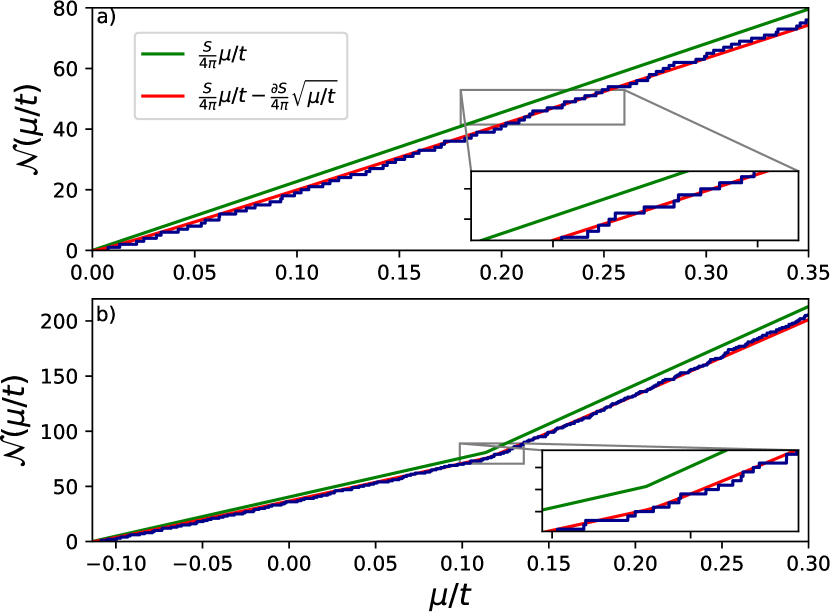
Figure 2: (Color online) $\mathcal{N}(\mu/t)$ for a ballistic quarter stadium MB (see Fig. 1c. The solid lines are obtained using Eq. (10) for the top panel and Eq. (17) for the bottom panel, as a function of $\mu/t$. The green line refers to the first term in the Weyl expansion whereas the red line includes the surface corrections. The staircase plot (blue line) is the result of tight-binding simulations. Lower-right insets are zoom-ins to show the fit between tight-binding simulation and theory. a) p-wave Majorana billiard with with $L=80a$, $W=40a$ and $\Delta^{\prime}=0.001ta$. b) s-wave MB with $L=100a$, $W=50a$, $B=0.23t$, $\Delta=0.2t$ and $\alpha=0.001ta$. The kink in the plot is at $\mu=\epsilon$ and signals the entrance of the second spin band, previously spin-polarized, into the picture.

In this section, we investigate the density of FPXs for p- and s-wave topological superconductors. We show that the FPX points of $H_{p}$ and $H_{s}$ are real eigenvalues of a corresponding non-Hermitian operator (Eqs. (7) and (12)). Further simplification is possible if $S\ll\xi\partial S$, where $S$ is the system area, $\partial S$ is the size of the boundary and $\xi$ is the superconducting coherence length. (For example, for a rectangular cavity of width $W$, this limit corresponds to $W\ll\xi$ .) In this limit, the non-Hermitian eigenvalue problem for $H_{p}$ and $H_{s}$ can be transformed by a local rescaling transformation to a Hermitian eigenvalue problem (Eqs. (9) and (15)). We thus show that, surprisingly, the FPX points of MBs are related to the energy eigenvalues of a Hermitian operator which we identify as the normal state Hamiltonian. We next derive the Weyl expansion for the average density of FPXs, which is expressed in Eqs. (10) and (17) for the p- and s-wave cases, respectively. We also perform numerical tight-binding simulations, which we detail in Appendix A, and compare our results with our formulae. We present our results for a 2D Majorana billiard in Figs. 2a and b, where we plot the integrated density of FPXs $\mathcal{N}(\mu/t)$ for p- and s-wave systems. We see that the analytical and numerical results fit remarkably well without any fitting parameters, once the boundary corrections in the Weyl expansion are taken into account.

III.1 Average density of FPXs of a p-wave Majorana billiard

We first focus on the FPXs of a p-wave Majorana billiard described by the Hamiltonian $H_{p}$ (Eq. (2)). In this case, there’s only a single external parameter, namely the chemical potential, to be varied, hence $\beta=\mu/t$. The FPX points are the $\mu_{i}$ values for which the p-wave h Hamiltonian has a zero-energy eigenstate:

$$H_{p}|_{\mu=\mu_{i}}\,\chi =0.$$ (6)

We map the problem of finding the FPX points to that of finding eigenvalues of a non-Hermitian operator by premultiplying Eq. (6) by $\tau_{z}$:

$$\Bigg{(}\frac{\big{(}\mathbf{p}+im\Delta^{\prime}\boldsymbol{\eta}\big{)}^{2}}{2m}+V(\mathbf{r})+m\Delta^{\prime 2}\Bigg{)}\chi =\mu\,\chi,$$ (7)

where $\boldsymbol{\eta}=\tau_{y}\hat{x}-\tau_{x}\hat{y}$. We identify this operator as the Hamiltonian of a Rashba 2DEG with an imaginary Rashba parameter $\alpha=i\Delta^{\prime}$. Eq. (7) shows that the real right-eigenvalues of this non-Hermitean operator correspond to the FPX points, whereas the complex eigenvalues are associated with avoided crossings.

There is no general reason to assume that a given right-eigenvalue of Eq. (7) is real. However, further simplification is possible in the limit of $S/\partial S\ll\xi=\hbar/m\Delta^{\prime}$. Rescaling the eigenfunction $\chi={\rm e}^{\boldsymbol{\eta}\cdot\mathbf{r}/\xi-r^{2}/\xi^{2}}\tilde{\chi}$ and expanding in powers of $S/(\xi\,\partial S)$, we obtain REF:Adagideli14

$$\Bigg{(}\frac{\big{(}\mathbf{p}+\frac{2m^{2}\Delta^{\prime 2}}{\hbar}(\hat{\mathbf{z}}\times\mathbf{r})\,\tau_{z}\big{)}^{2}}{2m}+V(\mathbf{r})+m\Delta^{\prime 2}\Bigg{)}\,\tilde{\chi} =\mu\,\tilde{\chi}.$$ (8)

We see that the crossing points are eigenvalues of the normal state Hamiltonian with a fictitious magnetic field $\pm 2m^{2}(\Delta^{\prime})^{2}/e\hbar$ and a constant potential shift $m(\Delta^{\prime})^{2}$. We further note that the energy levels are even functions of applied magnetic fields. Therefore, to the order we are working in, the effect of the fictitious magnetic field on the crossing points can be ignored, as they only serve to modify the nonzero split in energy levels. Hence we see that all eigenvalues of Eq. (8) are real. We thus arrive at the remarkable result that all FPX points are simply eigenvalues of a normal state Hamiltonian:

$$\left(\frac{p^{2}}{2m}+V(\mathbf{r})+m\Delta^{\prime 2}\right)\,\tilde{\chi} =\mu\tilde{\chi}.$$ (9)

This identification allows us to map the average density of FPXs to the conventional density of states of a normal state Hamiltonian. Well known results, such as the Weyl expansion for average DOS REF:Book:Weyl68 ; REF:Balian70 ; REF:Book:Baltes76 (or, for the case of soft confinement, the Thomas-Fermi approximation REF:Book:Brack03 ); Gutzwiller’s trace formula in billiards for oscillations (supershell effects) in DOS REF:Book:Gutzwiller90 ; REF:Jalabert90 ; REF:Ishio95 ; REF:Adagideli02a ; REF:Adagideli02 ; the theory of Lifshitz tails REF:Lifshitz64 ; REF:Halperin65 ; REF:BOOK:Itzykson89 for disordered systems; as well as the random matrix theory results for DOS fluctuations REF:Beenakker97 ; REF:Beenakker13b , carry over to the spectra of fermion-parity crossings.

For the average density of FPXs for the p-wave system $\bar{\rho}_{\textrm{w},p}(\mu)$ in $d$ dimensions, we thus obtain REF:Footnote:3DDoFPX :

$$\bar{\rho}_{\textrm{w},p}(\mu) =\begin{cases}\frac{L}{2\pi\sqrt{\mu}}+\mathcal{O}(1)&\textrm{if }d=1\\ \frac{S}{4\pi}-\frac{\partial S}{8\pi\sqrt{\mu}}&\textrm{if }d=2\\ \frac{V\sqrt{\mu}}{4\pi^{2}}-\frac{\partial V}{16\pi}&\textrm{if }d=3,\end{cases}$$ (10)

where $L$ is the length of the 1D wire, $S$ and $\partial S$ are the area and perimeter of the 2D billiard, and $V$ and $\partial V$ the volume and surface area of the 3D dot cavity respectively.

III.2 Average density of FPXs of a s-wave Majorana billiard

We now focus on the FPXs of an s-wave Majorana billiard described by $H_{s}$ (Eq. (1)). In this case, there are two external parameters, namely the chemical potential and the Zeeman energy. Hence $\beta$ can be either $\mu/t$ or $B/t$. We again start with the zero energy eigenvalue problem

$$H_{s}|_{\mu_{i},B_{j}}\,\psi =0$$ (11)

where $\mu_{i}$ and $B_{j}$ are the FPX points. Here, we have two equivalent choices of obtaining a non-Hermitian eigenvalue problem: eigenvalues corresponding to $B$ or to $\mu$. This equivalence leads to a scaling relation between $\mu_{i}$ and $B_{j}$ which we discuss in Section III.3. Without loss of generality we focus on the eigenvalue problem for $\mu_{i}$ below. We premultiply Eq. (11) with $\tau_{z}$ and obtain

$$\left(\frac{\mathbf{p}^{2}}{2m}+V(\mathbf{r})+\alpha\boldsymbol{\eta}\cdot\mathbf{p}+B\sigma_{x}\tau_{z}+i\Delta\tau_{y}\right)\psi =\mu\,\psi,$$ (12)

where $\boldsymbol{\eta}=(\sigma_{y}\hat{x}-\sigma_{x}\hat{y})$. This equation can then be solved using tight binding methods, see appendix A.

In order to proceed analytically, we follow Ref. [REF:Adagideli14, ] and [REF:Pekerten17, ] to again transform the usual eigenvalue problem ($H_{s}\,\psi=E\,\psi$ with $E=0$) to a non-Hermitian eigenvalue problem and obtain:

$$\left(h(\mathbf{p},\mathbf{r})\sigma_{z}-i\alpha p_{x}\sigma_{x}\mp B\mp\Delta\sigma_{x}\right)\,\phi_{\pm} =0.$$ (13)

Here, we have ignored the chiral symmetry breaking term $i\alpha p_{y}\sigma_{y}$, which is justified in the limit $S\ll\xi\partial S$, as in the previous section. For a finite system, the solution that satisfies all boundary conditions can be expressed as

$$\phi_{n,\pm}=\zeta_{\pm}(E_{n}){\rm e}^{\pm x/\xi}\psi_{n},$$ (14)

where $\zeta_{\pm}(\epsilon)$ are the eigenvectors of the $2\times 2$ matrix $\epsilon\,\sigma_{z}\mp\Delta\sigma_{x}$ with eigenvalue $\pm\sqrt{\epsilon^{2}+\Delta^{2}}$ and $\psi_{n}$ satisfies the eigenvalue equation:

$$h\,\psi_{n} =E_{n}\,\psi_{n}.$$ (15)

Substituting Eq. (14) into Eq. (13), we find that the zero mode solutions (hence the fermion-parity crossings) happen on families of curves in the $B-\mu$ plane. The curves satisfy

$$B^{2}=(\mu-E_{n})^{2}+\Delta^{2}$$ (16)

for a given eigenvalue $E_{n}$ of the spinless single particle Hamiltonian $h(\mathbf{p},\mathbf{r})$. Hence, the density of FPX spectrum (with respect to either $\mu$ or $B$) can be obtained by analyzing the set of eigenvalues $\{E_{n}\}$ of $h(\mathbf{p},\mathbf{r})$. Noting that $h(\mathbf{p},\mathbf{r})$ is the same for s- and p-wave cases, we write the s-wave Weyl expansion for $\rho_{\textrm{w},s}(\mu)$ and $\rho_{\textrm{w},s}(B)$ for fermion-parity crossing densities in terms of their p-wave counterpart $\rho_{\textrm{w},p}(\mu)$ in Eq. (10):

$$\rho_{\textrm{w},s}(\mu,B)=\sum_{\varsigma=\pm 1}\rho_{\textrm{w},p}(\mu+\varsigma\epsilon)\,\theta(\mu+\varsigma\epsilon),$$ (17)

where $\theta(x)$ is the Heaviside step function, $\epsilon=\sqrt{B^{2}-\Delta^{2}}$ as before and the $\varsigma=\pm 1$ terms in the sum correspond to the densities of different spin species separated in energy by the Zeeman field.

III.3 Universal scaling properties of fermion-parity crossing points in s-wave systems

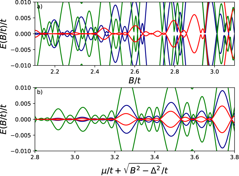
Figure 3: (Color online) A plot of the lowest four eigenvalues of the disordered s-wave Hamiltonian in Eq. (1), discretized on a 1D lattice of 100 sites, plotted as a function of (a) $B/t$ and (b) $\mu/t+\sqrt{B^{2}-\Delta^{2}}/t$, for different values of Hamiltonian parameters. In both plots, the green set of curves represents the lowest four eigenvalues obtained for $\Delta=1.5t$, $\alpha=0.05ta$, $\mu=1.8t$; the blue set is for $\Delta=1.8t$, $\alpha=0.05ta$, $\mu=2.0t$; and the red set is for $\Delta=1.8t$, $\alpha=0.08ta$, $\mu=1.6t$. In all cases, the same disorder realization with a disorder strength $V_{d}=0.5t$ is utilized.

As a consequence of Eq. (16), the FPX spectra exhibit a scaling relation for a given disorder realization: all the FPXs corresponding to different values of $\mu$, $B$ or $\Delta$, collapse on the same set of points if expressed in terms of the combination $\mu\pm\sqrt{B^{2}-\Delta^{2}}$ (Fig. 3). Moreover, if the FPX spectrum of one of the Zeeman-split spin bands is known, the other can immediately be determined by shifting the spectrum by $2\sqrt{B^{2}-\Delta^{2}}$.

This universality is evident in Fig. 3, where we plot the first four eigenvalues of a 1D s-wave system with a specific disorder realization for different values of $\mu$ and $\Delta$ as a function of $B$ in Fig. 3a and as a function of $\mu+\sqrt{B^{2}-\Delta^{2}}$ in Fig. 3b. These plots are obtained by discretizing the s-wave Hamiltonian in Eq. (1) in 1D over $100$ sites and numerically solving the resulting eigenvalue problem. We see that in Fig. 3b, all energy level crossings happen at the same set of values of $\mu+\sqrt{B^{2}-\Delta^{2}}$ for systems with the same disorder realization but different system parameters.

III.4 Lifshitz tail in disordered MBs

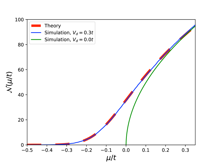
Figure 4: (Color online) $\mathcal{N}(\mu/t)$ vs. $\mu/t$ for a p-wave 1D MB for a wire of length $500a$ and $\Delta^{\prime}=0.001ta$. For the disordered case, the tight-binding simulation plot is the average of $200$ disorder realizations. The theory lines are the plots of Eq. (18) for $V_{d}=0$ and $V_{d}=0.3t$.

Disordered systems feature states below zero energy due to the presence of islands with an average of below zero potential, even though the average potential for the whole system is zero. Called the Lifshitz tail REF:Lifshitz64 ; REF:Halperin65 ; REF:BOOK:Itzykson89 , this phenomenon is also present in density of FPXs in MBs (see Fig. 4). The overall disorder-averaged integrated density of FPXs $\mathcal{N}(\mu/t)$ for a 1D p-wave MB with Gaussian disorder (i.e. $\left\langle V(\mathbf{r})V(\mathbf{r}^{\prime})\right\rangle=D\,\delta(\mathbf{r}-\mathbf{r}^{\prime})$ ) is given by the formula REF:BOOK:Itzykson89 :

$$\mathcal{N}(\mu) =\frac{\kappa_{0}}{\pi^{2}\,\varepsilon_{0}}\,\frac{1}{[\textrm{Ai}(-2\mu/\varepsilon_{0})]^{2}+[\textrm{Bi}(-2\mu/\varepsilon_{0})]^{2}},$$ (18)

where Ai and Bi are the Airy functions, $\varepsilon_{0}=(D^{2}\,m\hbar^{-2})^{1/3}$ and $\kappa_{0}=(D\,m^{2}\hbar^{-4})^{1/3}$.

In Fig. 4, we plot Eq. (18) and tight-binding simulations for a 1D disordered wire (and a tight-binding simulation for the same wire with zero disorder for comparison). We observe FPXs in the fully spin-polarized wire even in negative values of $\mu$, caused by rare disorder configurations. We note that the theory and the numerical simulations show remarkable agreement without any fitting parameters.

IV Oscillatory part of density of fermion-parity crossings

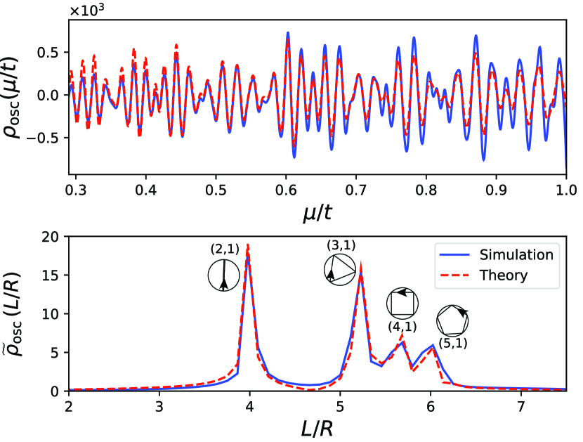
Figure 5: (Color online) a) Density oscillations of fermion-parity crossings $\rho_{\textrm{osc}}$ for a clean p-wave disk Majorana billiard with $R=100a$, $\Delta^{\prime}=0.001ta$. b) The Fourier transform of $\rho_{osc}$. The $(v,w)$ pairs and corresponding classical orbits for the peaks are labeled. The smoothing parameter for both figures is $\gamma=0.4/R$.

We next investigate the oscillatory part $\rho_{\rm osc}$ of the density of FPXs (see Eq. (5)). The DOS analog of such oscillations are the so-called shell and supershell effects known from the studies of finite quantum systems such as nuclei, atomic clusters and nanoparticles. The celebrated Guztwiller or Balian-Bloch trace formula show that each periodic orbit contributes a term oscillating with its classical action REF:Balian70 ; REF:Book:Gutzwiller90 ; REF:Jalabert90 ; REF:Ishio95 ; REF:Adagideli02a ; REF:Adagideli02 .

In this section, we extend the analysis of the oscillatory part of DOS in Ref. [REF:Balian70, ] and [REF:Book:Brack03, ] to the case of the FPX spectrum of a clean p-wave MB. We again take advantage of the mapping described in Section III.1 of the p-wave Hamiltonian to a normal state Hamiltonian with eigenvalues yielding the FPX points. We thus extend the Gutzwiller and/or Balian Bloch trace formula REF:Balian70 ; REF:Book:Gutzwiller90 from its original setting of the DOS of finite systems into the FPXs of finite Majorana platforms. The new trace formula expresses the oscillating part $\rho_{\textrm{osc}}$ as a sum over classical periodic orbits $\zeta$. Its general form is

$$\rho_{\textrm{osc}}(\mu)=\sum_{\zeta}{\cal A}_{\zeta}\cos\Phi_{\zeta}(\mu),$$ (19)

where ${\cal A}_{\zeta}$ is related to the stability of the orbit and $\hbar\Phi_{\zeta}$ is related to its classical action as well as the Maslov indices. Their detailed form depends on whether the orbits are isolated or part of a family of orbits (sometimes called degenerate orbits). For isolated periodic orbits,

$${\cal A}_{\zeta}=\frac{T_{\zeta}/\pi\hbar}{\sqrt{|\det(M_{\zeta}-I)|}},\quad\Phi_{\zeta}(\mu)=\frac{S_{\zeta}(\mu)}{\hbar}-\frac{\sigma_{\gamma}\pi}{2},$$ (20)

where $T_{\zeta}$ is the period of the corresponding primitive periodic orbit (i.e. the parent orbit with no retracings), $M_{\zeta}$ is the stability matrix of the orbit REF:FOOTNOTE:stabilityM and $\sigma_{\gamma}$ is the Maslov index. The final ingredient is the classical action, given by $S_{\zeta}(\mu)=\oint_{\zeta}\mathbf{p}\cdot d\mathbf{r}$. The weight of individual contributions increases for degenerate orbits. For two dimensional systems–which is our main focus–and singly degenerate orbits

$${\cal A}_{\zeta}=\frac{2m}{(2\pi\hbar)^{3/2}p_{F}}\int\left|\frac{\partial r_{\perp}}{\partial p^{\prime}_{\perp}}\right|^{-1/2}_{\zeta}dr_{\parallel}\,dr_{\perp}\,,$$

$$\Phi_{\zeta}(\mu)=\frac{S_{\zeta}(\mu)}{\hbar}-\frac{\sigma_{\gamma}\pi}{2}-\frac{\pi}{4},$$ (21)

where $p_{F}$ is the Fermi momentum. Here an initial transverse perturbation of momentum $p_{\perp}^{\prime}$ leads to a final transverse deviation $r_{\perp}$ after a full round. We note that in a billiard system $|\mathbf{p}|=p_{F}$, hence the classical action corresponding to a periodic orbit is $S_{\zeta}(\mu)=p_{F}L_{\zeta}$ where $L_{\zeta}$ is the length of the orbit $\zeta$.

In order to demonstrate our results, we specialize to a clean p-wave disk MB of radius $R$ (see Fig. 1). For this system, it is possible to obtain closed-form analytical formulae using Eq. (19) and compare the numerical simulations with these formulae. We first note that a periodic orbit of a disk billiard is uniquely determined by the number $w$ times the orbit winds around the billiard and the number $v$ times it reflects from the boundary. Then a simple geometrical consideration allows one to express the length of the orbit as $L_{vw}=2vR\sin(\pi w/v)$. We thus obtain

$$\rho_{\mathrm{osc}}(\mu) =\frac{2mR^{2}}{\hbar^{2}}\,\bigg{(}\frac{\hbar}{\pi R\,p(\mu)}\bigg{)}^{1/2}\,$$

$$\quad\times\sum_{w=1}^{\infty}\sum_{v=2w}^{\infty}f_{vw}\frac{\sin^{3/2}(\pi w/v)}{\sqrt{v}}$$

$$\quad\times\mathrm{Im}\bigg{[}\exp\bigg{\{}i\frac{p_{F}L_{vw}}{\hbar}+i\phi_{\textrm{po}}\bigg{\}}\bigg{]},$$ (22)

where $\phi_{\textrm{po}}=-3v\pi/2+3\pi/4$, $f_{vw}=2\,\theta(v-2w)$ with $\theta(x)$ being the Heaviside step function. In Fig. 5a, we plot $\rho_{\textrm{osc}}(\mu/t)$ as determined from numerical solutions of the Majorana billiard REF:Scharf2015 ; REF:FOOTNOTE:Scharf (blue, solid line) and as given by Eq. (IV) (red, dashed line) for a p-wave disk MB. Both lines are smoothed using a Gaussian smoothing function. The plots show remarkable agreement. In Fig. 5b, we plot the Fourier transform $\tilde{\rho}_{\textrm{osc}}(L/R)$ of Fig. 5a in order to observe the location of the periodic orbits and their relative amplitudes. (We choose to show the Fourier transform as a function of the dimensionless parameter $L/R$, i.e. orbit length divided by disk radius, rather than as a function of the period of the orbit for convenience, since the length and the period of a given orbit are proportional.) As discussed above, the peaks are centered around the $L/R$ values of the high-degeneracy orbits (shown in the insets) and their relative amplitude reflects their order of degeneracy.

It is a straightforward task to extend Eq. (IV) for the case of a generic (tight-binding) energy dispersion and obtain the corresponding $\rho_{\textrm{osc}}$, for details we refer the reader to Appendix B.

V Universal fluctuations of fermion-parity crossings

We now focus on how consecutive fermion-parity crossings are correlated. We first work in the limit $S/\partial S\ll\xi$ (i.e. one of the system size parameters (the “width”) becomes smaller than the superconducting coherence length) and we obtain the FPX spacing distributions. We find that the FPX points are uncorrelated for systems that are localized in their normal state and the spacing distribution is Poissonian:

$$P(\delta\mu)=\exp\big{(}-\delta\mu/\langle\delta\mu\rangle\big{)},$$ (23)

where $\delta\mu$ is the FPX spacing and $\langle\delta\mu\rangle$ is its ensemble-averaged value. When the normal state system is near a delocalization transition, the FPX points become correlated and feature antibunching for small spacings, while large spacings remain uncorrelated. This behaviour is reflected in the semi-Poissonian distribution, signaling the fractal nature of the wavefunction near the metal insulator transition REF:Shklovskii93 :

$$P(\delta\mu)=\frac{\delta\mu}{\langle\delta\mu\rangle}\exp\big{(}-2\delta\mu/\langle\delta\mu\rangle\big{)}.$$ (24)

Finally if the normal system is delocalized enough that the escape time is shorter than $\hbar/\langle\delta\mu\rangle$, the FPX points feature correlations that are reminiscent of the eigenvalues of an ensemble of real Hermitian random matrices and the corresponding distribution is the Wigner-Dyson distribution for orthogonal matrices REF:Wigner55 ; REF:Dyson62 ; REF:Dyson62b ; REF:Dyson63 ; REF:Beenakker97 ; REF:Book:Mehta04 :

$$P(\delta\mu)=\frac{\pi\delta\mu}{2\langle\delta\mu\rangle}\exp\bigg{(}-\frac{\pi\delta\mu^{2}}{4\langle\delta\mu\rangle^{2}}\bigg{)},$$ (25)

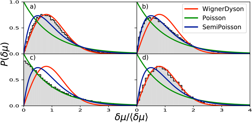
Figure 6: (Color online) a-c) Level spacing distributions for a disordered rectangular p-wave MBs of varying lengths, averaged over 500 disorder realizations, with $\Delta^{\prime}=0.025ta$, disorder strength $V_{d}=0.5t$, width $W=20a$. a) $L=40a<\xi$, b) $L=100a\gtrsim\xi$ and c) $L=1600a\gg\xi$, with $\xi=80a$ being the superconducting coherence length. d) Level spacing distributions, averaged over 225 cavity realizations, for a clean p-wave Lorentz cavity MB. Here, $\Delta^{\prime}=0.001ta$, $L=50a$, $W=50a$, and $r_{1}=r_{2}=10a$. The values of $L/\xi$ in panels a)-d) are $0.5$, $1.25$, $20$ and $0.4$, respectively.

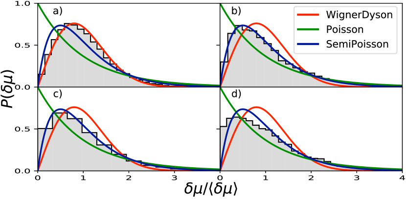
Figure 7: (Color online) a-c) Level spacing distributions for disordered rectangular s-wave MBs with increasing Zeeman energy $B$, averaged over 500 disorder realizations, with $L=200a$, $W=10a$, $V_{d}=0.2t$, $\alpha=0.025ta$, $\Delta=0.12t$, and a) $B=1.12t$, b) $B=0.22t$ and c) $B=0.13t$. d) Level spacing distributions for clean s-wave Lorentz cavity MB, averaged over 225 cavity realizations. Here, $\alpha=0.001ta$, $\Delta=0.2t$, $B=0.23t$, $L=50a$, $W=50a$, and $r_{1}=r_{2}=10a$. The values of $L/\xi$ in panels a)-d) are $0.27$, $1.63$, $6.1$ and $0.04$, respectively.

We again utilize a tight-binding model in order to numerically obtain the FPX spacings and plot the results against the distribution functions given in Eq. (23), (24) and (25). Fig. 6 [Fig. 7] shows our p-wave [s-wave] results for disordered rectangle cavities (a-c) and chaotic billiards (d). In agreement with our predictions, the distributions evolve from Wigner-Dyson to semi-Poissonian to Poissonian as the escape time is increased (the system becomes more localized), and fit the respective distributions well (see Fig. 6). We note, however, that in the s-wave case, $P(\delta\mu\rightarrow 0)$ approaches $0.5$ if both spin species are populated. This is due to FPX points constituting two interlaced sequences belonging to different spin species REF:Pekerten17 for larger $B$ (see Eq. (17)). While the elements of each sequence feature level repulsion, one sequence is the shifted version of the other. For large enough shifts, the two sequences become uncorrelated, hence the consecutive spacings between FPX of differing sequences will also be uncorrelated, suppressing the level repulsion.

Finally, we demonstrate a crossover between the universality classes in thin ($W\ll\xi$) 2D MBs as the system length $L$ is varied from being small to large with respect to $\xi$, hence modulating escape time relative to $\hbar/\langle\delta\mu\rangle$ and summarize the values of $L/\xi$ for the systems depicted in Figs. 6a-d and 7a-d. In Fig. 8, we note the locations of all of the Figs. 6a-d and 7a-d on the $L/\xi$ axis. All of these systems have one dimension (say, $W$) much smaller than $\xi$. However we stress that the numerical simulations depicted here do not use this approximation. The simulations use the full tight-binding version of the Bogoliubov–de Gennes Hamiltonian (see Appendix A).) Fig. 8 clearly shows the universality crossover in these systems.

The short coherence length limit, where the system size exceeds $\xi$ in all directions, was considered by Beenakker et al. REF:Beenakker13b In this case the FPX points have the same statistics as real eigenvalues of a real non-Hermitian matrix. For completeness, we also present the FPX spacing statistics in this limit in Fig. 9, where we show the statistics of a system with both dimensions $L_{1}$ and $L_{2}$ much larger than $\xi$, corresponding to a real Hamiltonian with semi-Poissonian statistics.

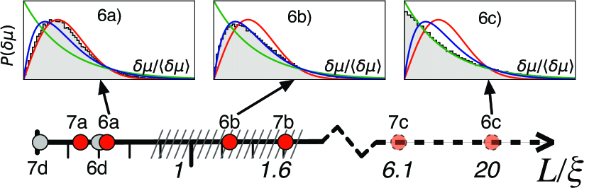
Figure 8: (Color online) The $L/\xi$ values for Figs. 6a-d and 7a-d. The shaded region on the $L/\xi$ axis around $L/\xi=1$ schematically represents the universality crossover region where the statistics are semi-Poissonian. Three panes from Fig. 6 are reproduced as an example of Gaussian, semi-Poissonian and Poissonian statistics. Here, $L$ for each shape is defined in Fig. 1.

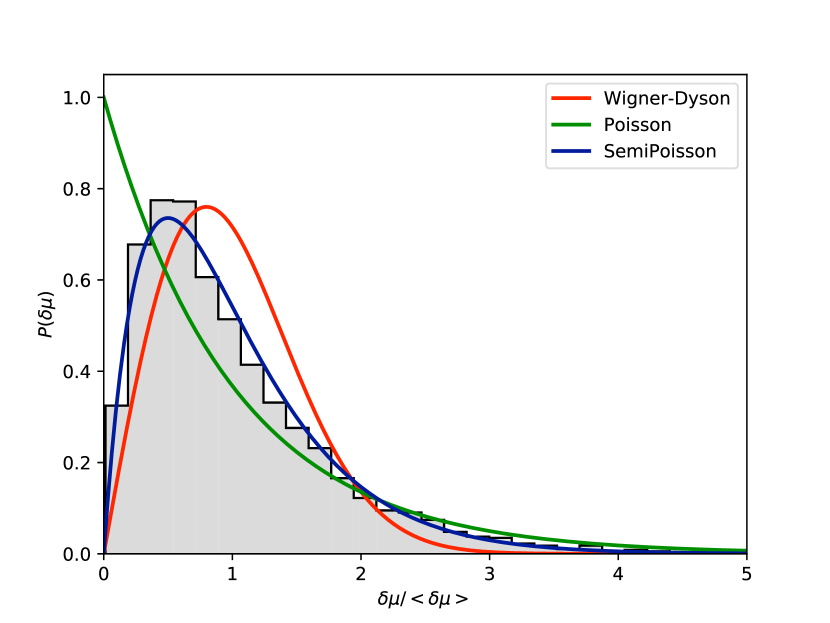
Figure 9: (Color online) Fermion-parity crossing spacing statistics for a p-wave system with both dimensions much larger than $\xi$ ($L=W=5\xi$), showing the statistics obtained from a tight-binding simulation of a disordered system in a square geometry (500 disorder realizations) whose parameters are $L=W=80a$, $V_{0}=0.32t$, $\Delta^{\prime}=0.125ta$ and $\xi=16a$.

VI Conclusions

In summary we studied the spectra of fermion-parity switches of a Majorana billiard using methods from semiclassical physics and quantum chaos. In particular, we show that the average density of fermion-parity crossings is described by a Weyl expansion and the disordered billiards feature Lifshitz tails in the fully depleted limit. Moreover, we demonstrate that the parity crossings has a tendency to sequentially bunch and anti-bunch, which is reminiscent of supershell effects in finite systems. We show that the oscillations in the density of fermion-parity crossings resulting from this bunching can be obtained by semiclassical means, extending Gutzwiller’s trace formula for conventional quantum billiards to Majorana billiards. Finally, we show that the fermion-parity crossing spacings obey a universal distribution as described by random matrix theory. We thus demonstrate that “one can hear (information about) the shape of a Majorana billiard” from fermion parity switches.

Appendix A Numerical tight-binding simulations

In order to demonstrate our analytical results in Sections III.1 and III.2 for average density of fermion-parity crossings, we perform tight-binding simulations of fermion-parity crossings in a p-wave and s-wave MBs using the Kwant toolbox for quantum transport REF:Kwant14 .

For the p-wave numerical results, we start with the LHS of Eq. (7), which is a non-Hermitian operator, as opposed to the p-wave Hamiltonian in Eq. (2). This non-Hermitean operator and the p-wave Hamiltonian in Eq. (2) are equivalent in the sense that no approximation was made in going from Eq. (2) to Eq. (7). We convert this non-Hermitean operator to its tight-binding form, which satisfies $\hat{O}_{\mathrm{TB}}^{\mathrm{PW}}\chi=\mu\chi$, using conventional methods (see, for example, Ref. [REF:Book:Datta97, ]):

$$\hat{O}_{\mathrm{TB}}^{\mathrm{PW}} =\big{(}2dt+V(x,y)\big{)}\,\tau_{0}\,\ket{x,y}\bra{x,y}$$

$$\qquad-t\tau_{0}\big{[}\ket{x+a,y}\bra{x,y}+\ket{x,y+a}\bra{x,y}+\mathrm{h.c.}\big{]}$$

$$\qquad+i\Delta^{\prime}\bigg{[}\frac{i}{2}\tau_{y}\ket{x+a,y}\bra{x,y}$$

$$\qquad\qquad-\frac{i}{2}\tau_{x}\ket{x,y+a}\bra{x,y}+\mathrm{h.c.}\bigg{]},$$ (26)

where $t=\hbar^{2}/2ma^{2}$ is the hopping parameter, $a$ is the lattice constant for the tight-binding lattice and $V(x,y)$ is the onsite potential. For disordered systems, we take the disorder to be Gaussian, i.e. $\left\langle V(\mathbf{r})V(\mathbf{r}^{\prime})\right\rangle=D\delta(\mathbf{r}-\mathbf{r}^{\prime})$ for $\mathbf{r},\mathbf{r}^{\prime}$ within the system, where $\left\langle\ldots\right\rangle$ represents averaging over disorder realizations, $D\equiv V_{d}^{2}a^{d}$ with $V_{d}$ being the disorder strength and $d$ is the dimension of the system. (In most of our manuscript, $d=2$; if $d=1$, then the hoppings in the $y$-direction are absent). In tight-binding simulations, this corresponds to choosing randomly the on-site potential from a Gaussian distribution. For ballistic cavity results, we set $V(x,y)=0$ within the cavity. The boundaries of the system are defined by the lack of hopping to outside. We form the tight-binding sparse matrix of this operator using the Kwant library REF:Kwant14 over the system shape described in Fig. 1 and the relevant plots. We then numerically obtain the eigenvalues of this (non-Hermitian) sparse matrix using LAPACK libraries present in the SciPy package REF:Scipy01 . We finally discard non-real eigenvalues to obtain our results.

For the s-wave results, we go through the same procedure, except for utilizing the appropriate tight-binding-representation of the non-Hermitian operator derived from the Hamiltonian in Eq. (1). For $E=0$, the tight-binding model for the s-wave equivalent of Eq. (7) reads $\hat{O}_{\mathrm{TB}}^{\mathrm{SW}}\chi=\mu\chi$, with the non-Hermitian operator $\hat{O}_{\mathrm{TB}}^{\mathrm{SW}}$ defined as:

$$\hat{O}_{\mathrm{TB}}^{\mathrm{SW}} =\big{[}\big{(}2dt+V(x,y)\big{)}\,\sigma_{0}\tau_{0}+B\,\sigma_{x}\tau_{z}\big{]}\,\ket{x,y}\bra{x,y}$$

$$\qquad-t\sigma_{0}\tau_{0}\big{[}\ket{x+a,y}\bra{x,y}+\ket{x,y+a}\bra{x,y}+\mathrm{h.c.}\big{]}$$

$$\qquad-\sigma_{y}\tau_{0}\,\big{[}\frac{i\alpha}{2}\,\ket{x+a,y}\bra{x,y}+\mathrm{h.c.}\big{]}$$

$$\qquad+\sigma_{x}\tau_{0}\,\big{[}\frac{i\alpha}{2}\,\ket{x,y+a}\bra{x,y}+\mathrm{h.c.}\big{]}$$

$$\qquad+i\Delta\sigma_{0}\tau_{y}\ket{x,y}\bra{x,y}.$$ (27)

Again, in the plots where $d=1$, the hoppings in the $y$-direction are absent.

For disorder averaging, we create many realizations of the same disordered system and do statistics over the combined results of each realization. For shape averaging over chaotic cavities, we create many realizations of the same chaotic cavity, the difference between realizations being the positioning of a relevant geometrical feature of the cavity, without changing the size of the system volume or boundary. For the Lorentz cavity, for example, we slightly change the position of the central stopper for each realization (making sure the stopper never comes too close to a wall). We check that the change is large enough numerically to yield a completely different set of eigenvalues.

Appendix B Oscillatory behavior of the density of fermion-parity crossings in a disk Majorana billiard

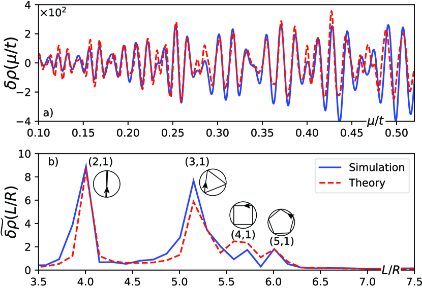
Figure 10: (Color online) a) Density oscillations of fermion-parity crossings $\rho_{\textrm{osc}}$ for a clean p-wave disk Majorana billiard on a lattice with $R=100a$, $\Delta^{\prime}=0.001ta$. b) The Fourier transform of $\rho_{osc}$. The $(v,w)$ pairs and corresponding classical orbits for the peaks are labeled. The smoothing parameter for both figures is $\gamma=0.4/R$.

In this section, we demonstrate the trace formula for $\rho_{\rm osc}$ (see Eq. (5)) for a p-wave disk MB of radius $R$. As opposed to the calculation in the main text, here we compare the trace formula to tight binding simulations.

We remind the reader that the oscillatory part $\rho_{\mathrm{osc}}(E)$ of the density of states $\rho(E)$ for a two dimensional disk billiard of radius $R$ with quadratic dispersion is given by REF:Book:Brack03 :

$$\rho_{\mathrm{osc}}(E) =\frac{1}{E_{0}}\sqrt{\frac{\hbar}{\pi pR}}\,\sum_{w=1}^{\infty}\sum_{v=2w}^{\infty}f_{vw}\frac{\sin^{3/2}(\varphi_{vw})}{\sqrt{v}}$$

$$\quad\times\mathrm{Im}\big{[}\exp\{i(S_{vw}/\hbar-3v\pi/2+3\pi/4)\}\big{]},$$ (28)

with

$$f_{vw}=\begin{cases}1&\mbox{if }v=2w\\ 2&\mbox{if }v>2w\end{cases}$$ (29)

and $E_{0}\equiv\hbar^{2}/(2mR^{2})$. For a quadratic Hamiltonian, $S_{vw}=p\,L_{vw}$ is the classical action of the orbit with $L_{vw}=2vR\sin(\varphi_{vw})$ being the classical orbit length of 2D disk, $\varphi_{vw}\equiv\pi w/v$ is half of the polar angle and $p$ is the momentum of the particle. As before, $v,w$ are two integers that correspond to the number of vertices and windings of the classical periodic orbit, respectively.

However the tight binding dispersion breaks the rotational symmetry of the problem weakly. The orbits that belong to the families that have the same action for a quadratic dispersion have slightly different actions for the tight binding dispersion. This type of symmetry breaking can then be treated by the semiclassical perturbation theory as discussed in REF:Book:Brack03 (see pp. 272). This would involve averaging the variation of the phases over all the orientations of the orbits, resulting in an effective dispersion $E_{\textrm{eff}}(p)$ of a fictitious rotationally invariant problem. We find that the (one dimensional tight-binding–like) dispersion $E_{\textrm{eff}}=2t\,(1-\cos{(pa/\hbar)})$ produces a very good fit to the numerical simulations. We thus obtain the expression for momentum $p(\mu)$:

$$p(\mu) =\frac{\hbar}{a}\arccos\bigg{(}1-\frac{\mu}{2t}\bigg{)}.$$ (30)

The deviations from the quadratic dispersion lead to a correction $S_{vw}\rightarrow S_{vw}+\Delta S_{vw}$ in the action:

$$\Delta S_{vw}=\frac{\hbar}{a}\tan\bigg{(}\frac{p(\mu)a}{2\hbar}\bigg{)}L_{vw}.$$ (31)

We now obtain the oscillatory part of the density of fermion-parity crossings corrected for tight binding dispersion:

$$\rho_{\mathrm{osc}}(\mu) =\frac{1}{E_{0}}\,\bigg{(}\frac{\hbar}{\pi R\,p(\mu)}\bigg{)}^{1/2}\,\sum_{w=1}^{\infty}\sum_{v=2w}^{\infty}f_{vw}\frac{\sin^{3/2}(\varphi_{vw})}{\sqrt{v}}$$

$$\quad\times\mathrm{Im}\bigg{[}\exp\bigg{\{}iL_{vw}$$

$$\qquad\times\,\bigg{(}\frac{p(\mu+i\gamma)}{\hbar}-\frac{1}{a}\,\tan\frac{p(\mu+i\gamma)\,a}{2\hbar}\bigg{)}$$

$$\quad+i\big{(}-3v\pi/2+3\pi/4\big{)}\bigg{\}}\bigg{]}.$$ (32)

Here, we combined Eq. (B), (30) and (31) at $\mu\rightarrow\mu+i\gamma$, with $\gamma$ being the smoothing parameter.

The numerical results for $\rho_{\mathrm{osc}}$ and $\widetilde{\rho}_{\mathrm{osc}}$ plotted in Fig. 10 is obtained by solving a tight-binding p-wave system shaped as a disk using the Kwant toolbox as described in Appendix A. We then obtain $\rho_{\mathrm{osc}}$ as

$$\rho_{\mathrm{osc}}(\mu/t) =\rho_{\gamma}(\mu/t)-\rho_{\textrm{w}}(\mu/t),$$ (33)

where $\rho_{\textrm{w}}$ corresponds to the volume and surface terms of the Weyl expansion in Eq. (10) and $\rho_{\gamma}$ is the smoothed density of fermion-parity crossings

$$\rho_{\gamma}(\mu/t) =\int d\mu^{\prime}\sum_{\mu_{c}}\delta(\mu^{\prime}-\mu_{c})\,F\bigg{(}\frac{\mu-\mu^{\prime}}{\gamma}\bigg{)},$$

$F\big{(}\frac{\mu-\mu^{\prime}}{\gamma}\big{)}$ is the Gaussian smoothing function with smoothing width $\gamma$. We then take the Fourier transform of $\rho_{\mathrm{osc}}(k(\mu/t)\,a)\xrightarrow{\mathrm{FT}}\widetilde{\rho}_{\mathrm{osc}}(L/R)$ to identify the peaks corresponding to the lowest length $L$ and the highest symmetry semiclassical periodic orbits REF:Book:Brack03 and plot the results in Fig. 10b. We find good agreement with our analytical results.

References

- (1) H. Weyl and K. Chandrasekharan Gesammelte Abhandlungen I, v.4 (Springer Berlin Heidelberg, 1968).
- (2) H. Baltes and E. Hilf, Spectra of finite systems: a review of Weyl’s problem, the eigenvalue distribution of the wave equation for finite domains and its applications on the physics of small systems (Bibliographisches Institut, 1976).
- (3) R. Balian and C. Bloch, Annals of Physics 60, 401 (1970).
- (4) M. Brack and R. K. Bhaduri, Semiclassical Physics, (Westview, Boulder, Colo., 2003).
- (5) R. Balian and C. Bloch, Annals of Physics 69, 76–160 (1972).
- (6) M. V. Berry, Proc. R. Soc. of London. Series A, Mathematical and Physical Sciences 400, 229 (1985).
- (7) M. C. Gutzwiller, Chaos in Classical and Quantum Mechanics, (Springer, New York, 1990).
- (8) M. Mehta, Random Matrices, Pure and Applied Mathematics (Elsevier Science, 2004).
- (9) J. Wurm, A. Rycerz, İ. Adagideli, M. Wimmer, K. Richter, and H. U. Baranger, Phys. Rev. Lett. 102, 056806 (2009).
- (10) E. P. Wigner, Annals of Mathematics 62, 548 (1955).
- (11) F. J. Dyson, Journal of Mathematical Physics 3, 1199 (1962).
- (12) F. J. Dyson, Journal of Mathematical Physics 3, 157–165 (1962).
- (13) F. J. Dyson and M. L. Mehta, Journal of Mathematical Physics 4, 701–712 (1963).
- (14) O. Bohigas, M. J. Giannoni, and C. Schmit, Phys. Rev. Lett. 52, 1 (1984).
- (15) A. V. Balatsky, I. Vekhter, and J.-X. Zhu, Rev. Mod. Phys. 78, 373 (2006).
- (16) S. Mi, D.I. Pikulin, M. Marciani, and C.W.J. Beenakker, J. Exp. Theor. Phys. 119, 1018 (2014).
- (17) L. Fu and C. L. Kane, Physical Review B 79, 161408(R) (2009).
- (18) S. Ryu, A. P. Schnyder, A. Furusaki, and A. W. W. Ludwig, New Journal of Physics 12, 065010 (2010).
- (19) T. D. Stanescu, R. M. Lutchyn, and S. Das Sarma, Phys. Rev. B 84, 144522 (2011).
- (20) E. J. H. Lee, X. Jiang, R. Aguado, G. Katsaros, C. M. Lieber, and S. De Franceschi, Phys. Rev. Lett. 109, 186802 (2012).
- (21) C. W. J. Beenakker, J. M. Edge, J. P. Dahlhaus, D. I. Pikulin, S. Mi, and M. Wimmer, Phys. Rev. Lett. 111, 037001 (2013).
- (22) M.-T. Rieder, P. W. Brouwer, and İ. Adagideli, Phys. Rev. B 88, 060509(R) (2013).
- (23) W. Chang, V. E. Manucharyan, T. S. Jespersen, J. Nygård, and C. M. Marcus, Phys. Rev. Lett. 110, 217005 (2013).
- (24) J. D. Sau and E. Demler, Phys. Rev. B 88, 205402 (2013).
- (25) D. M. Badiane, L. I. Glazman, M. Houzet, and J. S. Meyer, Comptes Rendus Physique 14, 840–856 (2013).
- (26) D. Chevallier, P. Simon, and C. Bena, Phys. Rev. B 88, 165401 (2013).
- (27) E. J. H. Lee, X. Jiang, M. Houzet, R. Aguado, C. M. Lieber, and S. De Franceschi, Nat. Nano. 9, 79 (2014).
- (28) S. Hegde, V. Shivamoggi, S. Vishveshwara, and D. Sen, New J. Phys. 17, 053036 (2015).
- (29) A. Y. Kitaev, Physics-Uspekhi 44, 131 (2001).
- (30) M. Z. Hasan and C. L. Kane, Rev. Mod. Phys. 82, 3045 (2010).
- (31) X.-L. Qi and S.-C. Zhang, Rev. Mod. Phys. 83, 1057 (2011).
- (32) J. Alicea, Reports on Progress in Physics 75, 076501 (2012).
- (33) B. A. Bernevig and T. Hughes Topological Insulators and Topological Superconductors (Princeton University Press, 41 William Street, Princeton, New Jersey 08540, 2013).
- (34) S. R. Elliott and M. Franz, Rev. Mod. Phys. 87, 137 (2015).
- (35) V. Mourik, K. Zuo, S. M. Frolov, S. R. Plissard, E. P. A. M. Bakkers and L. P. Kouwenhoven, Science 336, 1003 (2012).
- (36) S. Nadj-Perge, I. K. Drozdov, J. Li, H. Chen, S. Jeon, J. Seo, A. H. MacDonald, B. A. Bernevig and A. Yazdani, Science 346, 602 (2014).
- (37) A. Fornieri, A. M. Whiticar, F. Setiawan, E. P. Marín, A. C. C. Drachmann, A. Keselman, S. Gronin, C. Thomas, T. Wang, R. Kallaher, G. C. Gardner, E. Berg, M. J. Manfra, A. Stern, C. M. Marcus, and F. Nichele, Nature 569, 89–92 (2019).
- (38) S. Vaitiekėnas, M.-T. Deng, P. Krogstrup, and C. M. Marcus, arXiv:1809.05513 (2018).
- (39) T.H. Hsieh and L. Fu, Phys. Rev. Lett. 108, 107005 (2012).
- (40) E. Prada, P. San-Jose, and R. Aguado, Phys. Rev. B 86, 180503(R) (2012).
- (41) J.F. Silva and E. Vernek, Journal of Physics: Condensed Matter 28, 435702 (2016).
- (42) C.-X. Liu, J.D. Sau, T.D. Stanescu, and S. Das Sarma, Phys. Rev. B 96, 075161 (2017).
- (43) F. Nichele, A.C.C. Drachmann, A.M. Whiticar, E.C.T. O’Farrell, H.J. Suominen, A. Fornieri, T. Wang, G.C. Gardner, C. Thomas, A.T. Hatke, P. Krogstrup, M.J. Manfra, K. Flensberg, and C.M. Marcus, Phys. Rev. Lett. 119, 136803 (2017).
- (44) K. Zuo, V. Mourik, D.B. Szombati, B. Nijholt, D.J. van Woerkom, A. Geresdi, J. Chen, V.P. Ostroukh, A.R. Akhmerov, S.R. Plissard, D. Car, E.P.A.M. Bakkers, D.I. Pikulin, L.P. Kouwenhoven, and S.M. Frolov, Phys. Rev. Lett. 119, 187704 (2017).
- (45) H.-Z. Tang, Y.-T. Zhang, and J.-J. Liu, Physics Letters A 382, 991 (2018).
- (46) C. Moore, T.D. Stanescu, and S. Tewari, Phys. Rev. B 97, 165302 (2018).
- (47) M. Hell, K. Flensberg, and M. Leijnse, Phys. Rev. B 97, 161401(R) (2018).
- (48) C.-X. Liu, J. D. Sau, and S. Das Sarma, Phys. Rev. B 97, 214502 (2018).
- (49) A. Vuik, B. Nijholt, A.R. Akhmerov, and M. Wimmer, SciPost Physics 7, (2019).
- (50) C. Moore, C. Zeng, T.D. Stanescu, and S. Tewari, Phys. Rev. B 98, 155314 (2018).
- (51) C. Reeg, O. Dmytruk, D. Chevallier, D. Loss, and J. Klinovaja, Phys. Rev. B 98, 245407 (2018).
- (52) M. Kayyalha, M. Kargarian, A. Kazakov, I. Miotkowski, V.M. Galitski, V.M. Yakovenko, L.P. Rokhinson, and Y.P. Chen, Phys. Rev. Lett. 122, 047003 (2019).
- (53) J. Shen, S. Heedt, F. Borsoi, B. van Heck, S. Gazibegovic, R.L.M.O. het Veld, D. Car, J.A. Logan, M. Pendharkar, S.J.J. Ramakers, G. Wang, D. Xu, D. Bouman, A. Geresdi, C.J. Palmstrøm, E.P.A.M. Bakkers, and L.P. Kouwenhoven, Nat Commun 9, 1 (2018).
- (54) J. Chen, B. D. Woods, P. Yu, M. Hocevar, D. Car, S.R. Plissard, E.P.A.M. Bakkers, T. D. Stanescu, and S.M. Frolov, Phys. Rev. Lett. 123, 107703 (2019).
- (55) B. D. Woods, J. Chen, S.M. Frolov, and T.D. Stanescu, Phys. Rev. B 100, 125407 (2019).
- (56) Z. Cao, H. Zhang, H.-F. Lü, W.-X. He, H.-Z. Lu, and X.C. Xie, Phys. Rev. Lett. 122, 147701 (2019).
- (57) O. Motrunich, K. Damle, and D.A. Huse, Phys. Rev. B 63, 224204 (2001).
- (58) P.W. Brouwer, M. Duckheim, A. Romito, and F. von Oppen, Phys. Rev. B 84, 144526 (2011).
- (59) P.W. Brouwer, M. Duckheim, A. Romito, and F. von Oppen, Phys. Rev. Lett. 107, 196804 (2011).
- (60) D. I. Pikulin, J. P. Dahlhaus, M. Wimmer, H. Schomerus, and C. W. J. Beenakker, New Journal of Physics 14, 125011 (2012).
- (61) M. Popinciuc, V.E. Calado, X.L. Liu, A.R. Akhmerov, T.M. Klapwijk, and L.M.K. Vandersypen, Phys. Rev. B 85, 205404 (2012).
- (62) D. Bagrets and A. Altland, Phys. Rev. Lett. 109, 227005 (2012).
- (63) J. Liu, A. C. Potter, K. T. Law, and P. A. Lee, Phys. Rev. Lett. 109, 267002 (2012).
- (64) P. Neven, D. Bagrets, and A. Altland, New J. Phys. 15, 055019 (2013).
- (65) H. O. H. Churchill, V. Fatemi, K. Grove-Rasmussen, M. T. Deng, P. Caroff, H. Q. Xu, and C. M. Marcus, Phys. Rev. B 87, 241401(R) (2013).
- (66) J.D. Sau and S. Das Sarma, Phys. Rev. B 88, 064506 (2013).
- (67) H. Pan, W.S. Cole, J.D. Sau, and S. Das Sarma, arXiv:1906.08193 [cond-mat] (2019).
- (68) S. Das Sarma, J. D. Sau, and T. D. Stanescu, Phys. Rev. B 86, 220506(R) (2012).
- (69) R. Rodríguez-Mota, S. Vishveshwara, and T. Pereg-Barnea, J. Phys. Chem. Solids 128, 179-187 (2019).
- (70) These topological superconductor systems could be comprised of a finite-sized superconductor or a finite-sized normal-state region proximity coupled to a superconductor (also known as an Andreev billiard REF:Kostzin95 ; REF:Adagideli02a ; REF:Beenakker05 ).
- (71) M. Kac, The American Mathematical Monthly 73, 1 (1966).
- (72) Although isospectral domains of different shapes exist REF:Gordon92 , it turns out to be possible to extract geometrical and dynamical information from the energy spectra REF:Book:Weyl68 .
- (73) P. G. deGennes, Superconductivity of Metals and Alloys (Westview Press, 1999).
- (74) R. M. Lutchyn, J. D. Sau, and S. Das Sarma, Phys. Rev. Lett. 105, 077001 (2010).
- (75) Y. Oreg, G. Refael, and F. von Oppen, Phys. Rev. Lett. 105, 177002 (2010).
- (76) İ. Adagideli, M. Wimmer, and A. Teker, Phys. Rev. B 89, 144506 (2014).
- (77) R. A. Jalabert, H. U. Baranger, and A. D. Stone, Phys. Rev. Lett. 65, 2442 (1990).
- (78) H. Ishio and J. Burgdörfer, Phys. Rev. B 51, 2013 (1995).
- (79) İ. Adagideli and P. M. Goldbart, Phys. Rev, B 65, 201306(R) (2002).
- (80) İ. Adagideli and P. M. Goldbart, Int. J. Mod. Phys. B 16, 1381 (2002).
- (81) I M. Lifshitz, Advances in Physics 13, 483 (1964).
- (82) B. I. Halperin, Phys. Rev. 139, A104 (1965).
- (83) C. Itzykson and J.-M. Drouffe, Statistical Field Theory v.2 (Cambridge University Press, Cambridge [England]; New York, 1989).
- (84) C. W. J. Beenakker, Rev. Mod. Phys. 69, 731 (1997).
- (85) We note that the case in Eq. (10) is a trivial extension of the case in that the p-wave coupling term is considered to be a 2D coupling.
- (86) B. Pekerten, A. Teker, O. Bozat, M. Wimmer, and İ. Adagideli, Phys. Rev. B 95, 064507 (2017).
- (87) For a precise definition, see Appendix C of Ref. [REF:Book:Brack03, ].
- (88) We numerically solve Eq. (A6) of Ref. [REF:Scharf2015, ] for and thus obtain the set of ’s that allow a zero mode solution.
- (89) B. I. Shklovskii, B. Shapiro, B. R. Sears, P. Lambrianides, and H. B. Shore Phys. Rev. B 47 , 11487 (1993).
- (90) C. W. Groth, M. Wimmer, A. R. Akhmerov, and X. Waintal, New Journal of Physics 16, 063065 (2014).
- (91) S. Datta, Electronic Transport in Mesoscopic Systems (Cambridge University Presss, 1997).
- (92) E. Jones, E. Oliphant, P. Peterson et al. SciPy: Open Source Scientific Tools for Python (2001-) http://www.scipy.org/ [Online; accessed 2018-04-01].
- (93) I. Kosztin, D. L. Maslov, and P. M. Goldbart, Phys. Rev. Lett. 75, 1735 (1995).
- (94) C. W. J. Beenakker, in Quantum Dots: A Doorway to Nanoscale Physics, edited by W. Dieter Heiss (Springer Berlin Heidelberg, Berlin, Heidelberg, 2005), pp. 131–174.
- (95) C. Gordon, D. Webb, and S. Wolpert, Invent. Math 110, 1 (1992).
- (96) B. Scharf and I. Žutić, Phys. Rev. B 91, 144505 (2015).