Invariance Principle for the Random Lorentz Gas – Beyond the Boltzmann-Grad Limit

Abstract

We prove the invariance principle for a random Lorentz-gas particle in 3 dimensions under the Boltzmann-Grad limit and simultaneous diffusive scaling. That is, for the trajectory of a point-like particle moving among infinite-mass, hard-core, spherical scatterers of radius $r$, placed according to a Poisson point process of density $\varrho$, in the limit $\varrho\to\infty$, $r\to 0$, $\varrho r^{2}\to 1$ up to time scales of order $T=o(r^{-2}\left|{\log r}\right|^{-2})$. To our knowledge this represents the first significant progress towards solving rigorously this problem in classical nonequilibrium statistical physics, since the groundbreaking work of Gallavotti (1969) [gallavotti_69, gallavotti_70, gallavotti_99], Spohn (1978) [spohn_78, spohn_80] and Boldrighini-Bunimovich-Sinai (1983) [boldrighini-bunimovich-sinai_83]. The novelty is that the diffusive scaling of particle trajectory and the kinetic (Boltzmann-Grad) limit are taken simultaneously. The main ingredients are a coupling of the mechanical trajectory with the Markovian random flight process, and probabilistic and geometric controls on the efficiency of this coupling.

Similar results have been earlier obtained for the weak coupling limit of classical and quantum random Lorentz gas, by Komorowski-Ryzhik (2006) [komorowski-ryzhik_06], respectively, Erdős-Salmhofer-Yau (2007) [erdos-salmhofer-yau_08, erdos-salmhofer-yau_07]. However, the following are substantial differences between our work and these ones: (1) The physical setting is different: low density rather than weak coupling. (2) The method of approach is different: probabilistic coupling rather than analytic/perturbative. (3) Due to (2), the time scale of validity of our diffusive approximation – expressed in terms of the kinetic time scale – is much longer and fully explicit.

MSC2010: 60F17; 60K35; 60K37; 60K40; 82C22; 82C31; 82C40; 82C41

Key words and phrases: Lorentz-gas; invariance principle; scaling limit; coupling; exploration process.

Dedicated to Oliver Penrose on his 91st birthday.

1 Introduction

We consider the Lorentz gas with randomly placed spherical hard core scatterers in $\mathbb{R}^{d}$. That is, place spherical balls of radius $r$ and infinite mass centred on the points of a Poisson point process of intensity $\varrho$ in $\mathbb{R}^{d}$, where $r^{d}\varrho$ is sufficiently small so that with positive probability there is free passage out to infinity, and define $t\mapsto X^{r,\varrho}(t)\in\mathbb{R}^{d}$ to be the trajectory of a point particle starting with randomly oriented unit velocity, performing free flight in the complement of the scatterers and scattering elastically on them.

A major problem in mathematical statistical physics is to understand the diffusive scaling limit of the particle trajectory

$$t\mapsto\frac{X^{r,\varrho}(Tt)}{\sqrt{T}},\qquad\text{ as }\qquad T\to\infty.$$ (1)

Indeed, the Holy Grail of this field of research would be to prove the invariance principle (i.e. weak convergence to a Wiener process with nondegenerate variance) for the sequence of processes in (1) in either the quenched or annealed setting (discussed in section 1.1). For extensive discussion and historical background see the surveys [spohn_80, dettmann_14, marklof_14] and the monograph [spohn_91].

The same problem in the periodic setting, when the scatterers are placed in a periodic array and randomness comes only with the initial conditions of the moving particle, is much better understood, due to the fact that in the periodic case the problem is reformulated as diffusive limit of particular additive functionals of billiards in compact domains and thus heavy artillery of hyperbolic dynamical systems theory is efficiently applicable. In order to put our results in context, we will summarise very succinctly the existing results, in section 1.4.

There has been, however, no progress in the study of the random Lorentz gas informally described above, since the ground-breaking work of Gallavotti [gallavotti_69, gallavotti_70, gallavotti_99], Spohn [spohn_78, spohn_80] and Boldrighini-Bunimovich-Sinai [boldrighini-bunimovich-sinai_83] where weak convergence of the process $t\mapsto X^{r,\varrho}(t)$ to a continuous time random walk $t\mapsto Y(t)$ (called Markovian flight process) was established in the Boltzmann-Grad (a.k.a. low density) limit $r\to 0$, $\varrho\to\infty$, $r^{d-1}\varrho\to 1$, in compact time intervals $t\in[0,T]$, with $T<\infty$, in the annealed [gallavotti_69, gallavotti_70, gallavotti_99, spohn_78, spohn_80], respectively, quenched [boldrighini-bunimovich-sinai_83] setting.

Our main result (see Theorem 2 in subsection 1.3) proves the invariance principle in the annealed setting if we take the Boltzmann-Grad and diffusive limits simultaneously: $r\to 0$, $\varrho\to\infty$, $r^{d-1}\varrho\to 1$ and $T=T(r)\to\infty$. Thus while the diffusive limit (1) with fixed $r$ and $\varrho$ remains open, this is the first result proving convergence for times growing to infinity as $r\to 0$ in the setting of randomly placed scatterers, and hence it is a significant step towards the full resolution of the problem in the annealed setting.

1.1 The random Lorentz gas

We define now more formally the random Lorentz process. Place spherical balls of radius $r$ and infinite mass centred on the points of a Poisson point process of intensity $\varrho$ in $\mathbb{R}^{d}$, and define the trajectory $t\mapsto X^{r,\varrho}(t)\in\mathbb{R}^{d}$ of a particle moving among these scatterers as follows:

1. If the origin is covered by a scatterer then $X^{r,\varrho}(t)\equiv 0$.

2. If the origin is not covered by a scatterer then $t\mapsto X^{r,\varrho}(t)$ is the trajectory of a point-like particle starting from the origin with random velocity sampled uniformly from the unit sphere $S^{d-1}$ and flying with constant speed between successive elastic collisions on any one of the fixed, infinite mass scatterers.

The randomness of the trajectory $t\mapsto X^{r,\varrho}(t)$ (when not identically $0$) is due to two sources: the random placement of the scatterers and the random choice of initial velocity of the moving particle. Otherwise, the dynamics of the moving particle is fully deterministic, governed by classical Newtonian laws. With probability 1 (with respect to both sources of randomness) the trajectory $t\mapsto X^{r,\varrho}(t)$ is well defined.

Due to elementary scaling and percolation arguments

$$\mathbf{P}\big{(}\text{the moving particle is not trapped in a compact domain}\big{)}=\vartheta_{d}(\varrho r^{d}),$$ (2)

where $\vartheta_{d}:\mathbb{R}_{+}\to[0,1]$ is a percolation probability which is (i) monotone non-increasing; (ii) continuous except for one possible jump at a positive and finite critical value $u_{c}=u_{c}(d)\in(0,\infty)$; (iii) vanishing for $u\in(u_{c},\infty)$ and positive for $u\in(0,u_{c})$; (iv) $\lim_{u\to 0}\vartheta_{d}(u)=1$. We assume that $\varrho r^{d}<u_{c}$. In fact, in the Boltzmann-Grad limit considered in this paper (see (3) below) we will have $\varrho r^{d}\to 0$.

As discussed above, the Holy Grail of this field is a mathematically rigorous proof of the invariance principle of the processes (1) in either one of the following two settings.

1. Quenched limit: For almost all (i.e. typical) realisations of the underlying Poisson point process, with averaging over the random initial velocity of the particle. In this case, it is expected that the variance of the limiting Wiener process is deterministic, not depending on the realisation of the underlying Poisson point process.

2. Averaged-quenched (a.k.a. annealed) limit: Averaging over the random initial velocity of the particle and the random placements of the scatterers.

Remarks on the Hamiltonian character of the problem: We use a probabilistic language and setting in this paper, previously much of the literature has chosen to work in the Hamiltonian setting [gallavotti_69, gallavotti_70, gallavotti_99, spohn_78, spohn_80]. However, we should emphasise that this probabilistic description is equivalent to the annealed setting of a Hamiltonian system: The Lorentz particle moves according to Newton’s Second Law in the potential field of spherical hard core scatterers centred in the points of a Poisson Point Process. The potential field is

$$\Phi^{r,\varrho}(x):=\sum_{q\in\omega_{\varrho}}\varphi((x-q)/r),$$

where $\omega_{\varrho}$ is the realisation of a Poisson Point Process of intensity $\varrho$ in $\mathbb{R}^{d}\setminus B_{0,r}$ (that is, no scatterer within distance $r$ from the origin) and $\varphi(x):=\infty\mathbbm{1}_{\{\left|{x}\right|<1\}}$ is a spherical hard-core potential. The Hamiltonian equations of motion of the Lorentz particle are formally written as follows

$$\dot{X}^{r,\varrho}(t)=V^{r,\varrho}(t),\qquad\dot{V}^{r,\varrho}(t)=-\operatorname{grad}\Phi^{r,\varrho}(X^{r,\varrho}(t)),$$

with initial conditions

$$X^{r,\varrho}(0)=0,\qquad V^{r,\varrho}(0)\in S^{d-1}.$$

However, since the interaction potential is hard core, the equations of motion are singular and should be taken with a grain of salt.

1.2 The Boltzmann-Grad limit

The Boltzmann-Grad limit is the following low (relative) density limit of the scatterer configuration:

$$r\to 0,\qquad\qquad\varrho\to\infty,\qquad\qquad\varrho r^{d-1}\to v_{d-1},$$ (3)

where $v_{d-1}$ is the area of the $(d-1)$-dimensional unit disc. In this limit the expected free path length between two successive collisions will be 1. Other choices of $\lim\varrho r^{d-1}\in(0,\infty)$ are equally legitimate and would change the limit only by a time (or space) scaling factor.

It is not difficult to see that in the averaged-quenched setting and under the Boltzmann-Grad limit (3) the distribution of the first free flight length starting at any deterministic time, converges to an $EXP(1)$ and the jump in velocity after the free flight happens in a Markovian way with transition kernel

$$\mathbf{P}\big{(}v_{\texttt{out}}\in dv^{\prime}\bigm{|}v_{\texttt{in}}=v\big{)}=\sigma(v,v^{\prime})dv^{\prime},$$ (4)

where $dv^{\prime}$ is the surface element on $S^{d-1}$ and $\sigma:S^{d-1}\times S^{d-1}\to\mathbb{R}_{+}$ is the normalised differential cross section of a spherical hard core scatterer, computable as

$$\sigma(v,v^{\prime})=\frac{1}{4v_{d-1}}\left|{v-v^{\prime}}\right|^{3-d}.$$ (5)

Note that in $3$-dimensions the transition probability (4) of velocity jumps is uniform. That is, the outgoing velocity $v_{\tt{out}}$ is uniformly distributed on $S^{2}$, independently of the incoming velocity $v_{\tt{in}}$.

It is intuitively compelling but far from easy to prove that under the Boltzmann-Grad limit (3)

$$\Big{\{}t\mapsto X^{r,\varrho}(t)\Big{\}}\Rightarrow\Big{\{}t\mapsto Y(t)\Big{\}},$$ (6)

where the symbol $\Rightarrow$ stands for weak convergence (of probability measures) on the space of continuous trajectories in $\mathbb{R}^{d}$, see [billingsley_68]. The process $t\mapsto Y(t)$ on the right hand side is the Markovian random flight process consisting of independent free flights of $EXP(1)$-distributed length, with Markovian velocity changes according to the scattering transition kernel (4). A formal construction of the process $t\mapsto Y(t)$ is given in section 2.1. The limit (6), valid in any compact time interval $t\in[0,T]$, $T<\infty$, is rigorously established in the averaged-quenched setting in [gallavotti_69, gallavotti_70, gallavotti_99, spohn_78, spohn_80], and in the quenched setting in [boldrighini-bunimovich-sinai_83]. In [spohn_78] more general point processes of the scatterer positions, with sufficiently strong mixing properties are considered.

The limiting Markovian flight process $t\mapsto Y(t)$ is a continuous time random walk. Therefore, by taking a second, diffusive limit after the Boltzmann-Grad limit (6), Donsker’s theorem (see [billingsley_68]) yields indeed the invariance principle,

$$\Big{\{}t\mapsto T^{-1/2}Y(Tt)\Big{\}}\Rightarrow\Big{\{}t\mapsto W(t)\Big{\}},$$ (7)

as $T\to\infty$, where $t\mapsto W(t)$ is the isotropic Wiener process in $\mathbb{R}^{d}$ of non-degenerate variance. The variance of the limiting Wiener process $W$ can be explicitly computed but its concrete value has no importance.

The natural question arises whether one could somehow interpolate between the double limit of taking first the Boltzmann-Grad limit (6) and then the diffusive limit (7) and the plain diffusive limit for the Lorentz process, (1). Our main result, Theorem 2 formulated in section 1.3 gives a positive partial answer in dimension 3. Since our results are proved in three-dimensions from now on we formulate all statements in $d=3$ rather than general dimension. However, in some comments we will refer to general dimension $d$, when appropriate.

1.3 Results

In the rest of the paper we assume $\varrho=\varrho(r)=\pi r^{-2}$ and drop the superscript $\varrho$ from the notation of the Lorentz process.

Our results (Theorems 1 and 2 formulated below) refer to a coupling – joint realisation on the same probability space – of the Markovian random flight process $t\mapsto Y(t)$, and the quenched-averaged (annealed) Lorentz process $t\mapsto X^{r}(t)$. The coupling is informally described later in this section and constructed with full formal rigour in section 2.2.

The first theorem states that in our coupling, up to time $T\ll r^{-1}$, the Markovian flight and Lorentz exploration processes stay together.

Theorem 1.

Let $T=T(r)$ be such that $\lim_{r\to 0}T(r)=\infty$ and $\lim_{r\to 0}rT(r)=0$. Then

$$\lim_{r\to 0}\mathbf{P}\big{(}\inf\{t:X^{r}(t)\not=Y(t)\}\leq T\big{)}=0.$$ (8)

Remarks on Theorem 1: This result flashes some light on the strength of the probabilistic coupling method employed in this paper. In particular, with some elementary, purely probabilistic arguments it provides a formally stronger result than [gallavotti_69, gallavotti_70, gallavotti_99, spohn_78] which state the weak limit (6) (which follows from (8)) for any fixed $T<\infty$. Note, however, that complementing the cited papers with explicit error bounds (which seems feasible) would give Theorem 1. So, Theorem 1 on its own is a complement to these fundamental results. The full strength of our method is truly exhibit in Theorem 2, our main result, which extends this result to time scales where nontrivial correlations already appear. However the proof of Theorem 1 is included as it sheds light on the structure of the proof of Theorem 2.

Theorem 2.

Let $T=T(r)$ be such that $\lim_{r\to 0}T(r)=\infty$ and $\lim_{r\to 0}r^{2}\left|{\log r}\right|^{2}T(r)=0$. Then, for any $\delta>0$,

$$\lim_{r\to 0}\mathbf{P}\big{(}\sup_{0\leq t\leq T}\left|{X^{r}(t)-Y(t)}\right|>\delta\sqrt{T}\big{)}=0,$$ (9)

and hence

$$\Big{\{}t\mapsto T^{-1/2}X^{r}(Tt)\Big{\}}\Rightarrow\Big{\{}t\mapsto W(t)\Big{\}},$$ (10)

as $r\to 0$, in the averaged-quenched sense. On the right hand side of (10) $W$ is a standard Wiener process of variance $1$ in $\mathbb{R}^{3}$.

Indeed, the invariance principle (10) readily follows from the invariance principle for the Markovian flight process, (7), and the closeness of the two processes quantified in (9). So, it remains to prove (9). This will be the content of the larger part of this paper, sections LABEL:s:_Beyond_Naive-LABEL:s:_End_of_proof.

The point of Theorem 2 is that the Boltzmann-Grad limit of scatterer configuration (3) and the diffusive scaling of the trajectory are done simultaneously, and not consecutively. The memory effects due to recollisions and shading are controlled up to the time scale $T=T(r)=o(r^{-2}\left|{\log r}\right|^{-2})$.

Remarks on dimension: Our proof of Theorem 2 as it stands is valid in dimension $d=3$ only. We give here some comments on this fact and some hints on what can/could be proved by appropriate extensions of our method. However, we stress that any of these extensions would require some extra technical efforts. In order to keep the length of this paper under a reasonable limit, we do not include these arguments and extensions.

1. Issues in dimension $d=2$:

   1. Probabilistic estimates at the core of our proofs are valid (as stated and used) only in the transient dimensions of random walk, $d\geq 3$. This difference is implicit in the Green’s function estimates of sections LABEL:ss:_Bounds_-_Naive and LABEL:ss:_Bounds_for_Z. Nevertheless, with extra effort and the cost of an extra logarithmic factor (of order $\left|{\log r}\right|$) the estimates in section LABEL:ss:_Bounds_-_Naive, used in the proof of Theorem 1, can be saved in $d=2$, as well. Using these estimates (and relying on the Doeblin argument as hinted at in comment 2 below, Theorem 1, with a lorgarithmic factor, i.e. with $T(r)=o(r^{-1}\left|{\log r}\right|^{-1})$ turns out to be valid in $d=2$, as well.

   2. A subtle geometric argument which will show up in sections LABEL:ss:_Geometric_estimates-LABEL:ss:_Proof_of_Corollary_of_main-geom below, is valid only in $d\geq 3$, as well. This is unrelated to the recurrence/transience dichotomy and it is crucial in controlling the short range recollision and shadowing events, in the proof of Theorem 2.

2. The fact that in $d=3$ the differential cross section of hard spherical scatterers is uniform on $S^{d-1}$, c.f. (4), (5), facilitates our arguments, since, in this case, the successive velocities of the random flight process $Y(t)$ form an i.i.d. sequence. In dimensions $d\not=3$ this is not the case. However, this is a technical issue only, not of crucial importance in the argument. In dimensions $d>3$ the differential cross section (5) satisfies Doeblin’s condition $\inf_{v^{\prime}\in S^{d-1}}\sigma(v,v^{\prime})>0$ and, using Doeblin’s subtle trick, the sequence of successive velocities $(u_{n})_{n\geq 1}$ can be broken up in random i.i.d. blocks of exponentially tight lengths. This way, the main probabilistic steps of proof can be saved. In dimension $d=2$ Doeblin’s condition does not hold directly, see (5). However, it holds for the second convolution power $\sigma^{2}(v,v^{\prime}):=\int_{S^{d-1}}\sigma(v,v^{\prime\prime})\sigma(v^{\prime\prime},v^{\prime})dv^{\prime\prime}$ (that is, for the conditional distribution of velocity after two consecutive scatterings). In this way the sequence of successive velocities $(u_{n})_{n\geq 1}$ can be broken up in random 1-dependent strongly stationary (rather than i.i.d.) blocks of exponentially tight lengths. The necessary bounds can be proved with the use of Green’s function estimates for random walks with 1-dependent strongly stationary (rather than i.i.d.) steps.

3. Possible relation with singularity of the diffusion coefficient at $r\ll 1$ and certain limitations of our method:
   We state without proof the following estimates: In any dimension $d\geq 3$, there exist constants $C_{k}$, $k\geq 1$, such that

   $$\mathbf{P}\big{(}\inf_{t>\tau_{k}}\left|{Y(t)-Y(0)}\right|<r\big{)}\leq\begin{cases}C_{k}r^{k}&\text{ if \ }k\in[1,d-2],\\ C_{d-1}r^{d-1}\left|{\log r}\right|&\text{ if \ }k=d-1,\\ C_{k}r^{d-1}&\text{ if \ }k\in[d,\infty).\end{cases}$$

   In plain words, these are bounds on the probability of the continuous time random walk $t\mapsto Y(t)$ returning to the $r$-neighbourhood of its starting point, after $k$ or more scattering events. As we are not going to use these bounds in a technical sense we don’t prove them in this paper. The proof is not hard, however. We present these bounds for the following two reasons:

   1. The logarithmic factor in the case $k=d-1$ seems to be related to the expected singularity of the diffusion coefficient in the presumed (but not proved) diffusive limit (1), at $r\ll 1$.

   2. The fact that for $k\geq d$ the probability of recollision after $k$ scattering events is of order $r^{d-1}$, no matter how large $k$, is a clear warning about a limitation of our method, as is. Indeed, beyond time scales of order $T(r)\sim r^{-d+1}$ recollision patterns of all kinds of complexities occur, preventing any attempt of breaking up the time-line into quasi-independent legs, in a rigorously controlled way, as done in our proof. In conclusion, with hard work (in particular, hard geometric estimates) in dimension $d>3$ our proof could possibly be pushed up to time scales of order $T(r)=o(r^{-d+1}\left|{\log r}\right|^{-\alpha})$, with some $\alpha>0$, but certainly not further than this. Our proof of Theorem 2 reaches essentially this limit, in $d=3$. Going to time scales longer than $r^{-d+1}$ would require some genuinely new idea.

Remarks on robustness of the method: Our coupling method is robust, and could be applied to a variety of other interaction potentials with only technical and not conceptual extra difficulties. However, it does not seem to be easily extendable to point processes with correlations.

1. Extending our methods to non-spherical hard-core scatterers would change the differential cross-section (5). As such, the sequence of successive velocities of the $Y$-process would not be i.i.d. but a genuine Markov chain. However there are probabilistic methods to handle such difficulties (e.g. using Doeblin’s decomposition to independent blocks, as described in comment 2 above). For example, we quote the invariance principle for Ehrenfest’s wind-tree model (with hyper-cube scatterers), where - since the geometry is simpler - in a subsequent work we prove a result analogous to Theorem 2 for times of order $T(r)=o(r^{-2}\left|{\log r}\right|^{-1})$, c.f. [lutsko-toth_19].

2. Extension to smooth potentials can be done as well, though this is somewhat trickier. In this case, besides changing the differential cross section (5) one should also deal with non-instantaneous interactions. This can be handled in the case of finite range smooth potentials. The coupled Markov process will be different: not simple flights with instantaneous velocity jumps but flights with sharp but smooth scatterings. For details of the realisation of this coupling see the forthcoming work [helmuth-toth_20] where the weak coupling limit is pushed beyond the kinetic time scale with a similar, but not identical, probabilistic coupling method.

3. In the construction of the exploration process - as a Markov process - it is essential, however, that the point process where the scatterers are centred be Poisson. Otherwise, the exploration process could not be realised as a Markov process and probably would be of not much use. (Recall that in [spohn_78] the Boltzmann-Grad limit (6) is proved for point processes with certain correlations allowed.) This is certainly a limitation of our method. However, spatially inhomogeneous Poisson Point Processes could be handled.

Remarks on time scales: In various works the kinetic and diffusive limiting procedures are parametrised in different ways. We chose $r\to 0$, $\varrho=r^{-1/(d-1)}\to\infty$. In order to gauge how far beyond the bare kinetic limit the diffusive limit is pushed, and to compare our time scale with existing results on weak coupling diffusive limits, cf [komorowski-ryzhik_06, erdos-salmhofer-yau_08, erdos-salmhofer-yau_07] (see subsection 1.4 below for some details), we should introduce the kinetic time scale $T_{\mathrm{kin}}$. This is the space-time scale on which the kinetic limits [gallavotti_69, gallavotti_70, gallavotti_99, spohn_78, boldrighini-bunimovich-sinai_83, kesten-papanicolaou_80, erdos-yau_00, eng-erdos_05] hold, if formulated as scaling limit of the microscopic trajectory. In our notation it is

$$T_{\mathrm{kin}}:=\varrho^{1/d}=r^{-(d-1)/d}.$$ (11)

This time scale is the reference to which the time scale of validity of the diffusive limit should be gauged. In terms of the microscopic space-time - where typical spacing between scatterers is of order 1 and the Lorentz particle travels with velocity of order 1 - our diffusive limit holds for time scales up to

$$T_{\mathrm{diff}}=T_{\mathrm{kin}}T$$ (12)

with

$$T=o\left(r^{-2}\left|{\log r}\right|^{-2}\right)=o\left(T_{\mathrm{kin}}^{2d/(d-1)}(\log T_{\mathrm{kin}})^{-2}\right)\buildrel d=3\over{=}o\left(T_{\mathrm{kin}}^{3}(\log T_{\mathrm{kin}})^{-2}\right).$$ (13)

This is to be compared with the time scales of the similar-in-spirit classical [komorowski-ryzhik_06], respectively, quantum [erdos-salmhofer-yau_08, erdos-salmhofer-yau_07], weak coupling diffusive limits, cf. (16). See subsection 1.4 below for some details.

The proof of Theorems 1 and 2 will be based on a coupling (that is: a joint realisation on the same probability space) of the Markovian flight process $t\mapsto Y(t)$ and the averaged-quenched realisation of the Lorentz process $t\mapsto X^{r}(t)$, such that the maximum distance of their positions up to time $T$ be small order of $\sqrt{T}$. The Lorentz process $t\mapsto X^{r}(t)$ is realised as an exploration of the environment of scatterers. That is, as time goes on, more and more information is revealed about the position of the scatterers. As long as $X^{r}(t)$ traverses yet unexplored territories, it behaves just like the Markovian flight process $Y(t)$, discovering new, yet-unseen scatterers with rate 1 and scattering on them. However, unlike the Markovian flight process it has long memory, the discovered scatterers are placed forever and if the process $X^{r}(t)$ returns to these positions, recollisions occur. Likewise, the area swept in the past by the Lorentz exploration process $X^{r}(t)$ – that is: a tube of radius $r$ around its past trajectory – is recorded as a domain where new collisions can not occur. For a formal definition of the coupling see section 2.2. Let the associated velocity processes be $U(t):=\dot{Y}(t)$ and $V^{r}(t):=\dot{X}^{r}(t)$. These are almost surely piecewise constant jump processes. The coupling is realised in such a way, that

1. At the very beginning the two velocities coincide, $V^{r}(0)=U(0)$.

2. Occasionally, with typical frequency of order $r$ mismatches of the two velocity processes occur. These mismatches are caused by two possible effects:

   1. Recollisions of the Lorentz exploration process with a scatterer placed in the past. This causes a collision event when $V^{r}(t)$ changes while $U(t)$ does not.

   2. Scatterings of the Markovian flight process $Y(t)$ in a moment when the Lorentz exploration process is in the explored tube, where it can not encounter a not-yet-seen new scatterer. In these moments the process $U(t)$ has a jump discontinuity, while the process $V^{r}(t)$ stays unchanged. We will call these events shadowed scatterings of the Markovian flight process.

3. However, shortly after the mismatch events described in item B above, a new jointly realised scattering event of the two processes occurs, recoupling the two velocity processes to identical values. These recouplings occur typically at an $EXP(1)$-distributed time after the mismatches.

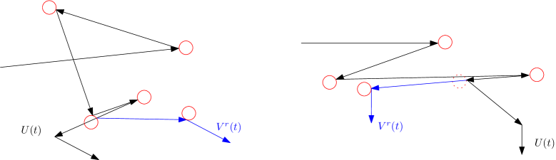
Figure 1: The above image shows a recollision (left) and a shadowing event (right). Note that after each event $U$ and $V^{r}$ are no longer coupled. However at the next scattering, if possible, the velocities are recoupled. On the right-hand-side the virtual scatterer drawn in dotted line is shadowed. That is: it is physically not present in the mechanical trajectory.

Summarising: The coupled velocity processes $t\mapsto(U(t),V^{r}(t))$ are realised in such a way that they assume the same values except for typical time intervals of length of order 1, separated by typical intervals of lengths of order $r^{-1}$. Other, more complicated mismatches of the two processes occur only at time scales of order $r^{-2}\left|{\log r}\right|^{-2}$. If the probability of all mismatches, and the separation associated to those that do occur, can be controlled (this will be the content of the proof) then the following holds:

Up to $T=T(r)=o(r^{-1})$, with high probability there is no mismatch whatsoever between $U(t)$ and $V^{r}(t)$. That is,

$$\lim_{r\to 0}\mathbf{P}\big{(}\inf\{t:V^{r}(t)\not=U(t)\}<T\big{)}=\lim_{r\to 0}\mathbf{P}\big{(}\inf\{t:X^{r}(t)\not=Y(t)\}<T\big{)}=0.$$ (14)

In particular, the invariance principle (10) also follows, with $T=T(r)=o(r^{-1})$, rather than $T=T(r)=o(r^{-2}\left|{\log r}\right|^{-2})$. As a by-product of this argument a new and handier proof of the theorem (6) of [gallavotti_69, gallavotti_70, gallavotti_99, spohn_78, spohn_80] also drops out.

Going up to $T=T(r)=o(r^{-2}\left|{\log r}\right|^{-2})$ needs more argument. The ideas exposed in the outline A, B, C above lead to the following chain of bounds:

$$\max_{0\leq t\leq 1}\left|{\frac{X^{r}(Tt)}{\sqrt{T}}-\frac{Y(Tt)}{\sqrt{T}}}\right|= \frac{1}{\sqrt{T}}\max_{0\leq t\leq 1}\left|{\int_{0}^{Tt}\left(V^{r}(s)-U(s)\right)ds}\right|$$

$$\leq \frac{1}{\sqrt{T}}\int_{0}^{T}\left|{V^{r}(s)-U(s)}\right|ds\asymp\frac{1}{\sqrt{T}}Tr=\sqrt{T}r.$$

In the $\asymp$ step we use the arguments B and C. Finally, choosing in the end $T=T(r)=o(r^{-2})$ we obtain a tightly close coupling of the diffusively scaled processes $t\mapsto X^{r}(Tt)/\sqrt{T}$ and $t\mapsto Y(Tt)/\sqrt{T}$, (9), and hence the invariance principle (10), for this longer time scale. This hand-waving argument should, however, be taken with a grain of salt: it does not show the logarithmic factor, which arises in the fine-tuning.

1.4 Summary of related work

In order to put our results in context we succinctly summarise the related most important results in the mathematically rigorous treatment of diffusion in the Lorentz gas. As Hendrik Lorentz’s seminal paper [lorentz_05] – where he proposes the periodic setting of what we call today the Lorentz gas for modelling diffusion and transport in solids – was published in 1905, and due to the large amount of work done in this field, we can not strive for exhaustion, and mention only a (possibly subjective) selection of the mathematically rigorous results. For more comprehensive historical overview we refer the reader to the survey papers [dettmann_14, marklof_14, spohn_80] and the monograph [spohn_91].

Scaling limit of the periodic Lorentz gas

As already mentioned, diffusion in the periodic setting is much better understood than in the random setting. This is due to the fact that diffusion in the periodic Lorentz gas can be reduced to the study of limit theorems of some particular additive functionals of billiard flows in compact domains. Heavy tools of hyperbolic dynamics provide the technical arsenal for the study of these problems.

The first breakthrough was the fully rigorous proof, by Bunimovish and Sinai [bunimovich-sinai_80], of the invariance principle (diffusive scaling limit) for the Lorentz particle trajectory in a two-dimensional periodic array of spherical scatterers with finite horizon. (Finite horizon means that the length of the straight path segments not intersecting a scatterer is bounded from above.) This result was extended by Chernov [chernov_94], to higher dimensions, under a still-not-proved technical assumption on singularities of the corresponding billiard flow.

In the case of infinite horizon (e.g. the plain $\mathbb{Z}^{d}$ arrangement of the spherical scatterers of diameter less than the lattice spacing) the free flight distribution of a particle flying in a uniformly sampled random direction has a heavy tail which causes a different type of long time behaviour of the particle displacement. The arguments of Bleher [bleher_92] indicated that in the two-dimensional case super-diffusive scaling of order $\sqrt{t\log t}$ is expected. For the Lorentz-particle displacement in the $2$-dimensional periodic case with infinite horizon, a central limit theorem with this anomalous scaling was proved with full rigour by Varjú and Szász [szasz-varju_07] and Dolgopyat and Chernov [dolgopyat-chernov_09]. The periodic infinite horizon case in dimensions $d\geq 3$ remains open.

Boltzmann-Grad limit of the periodic Lorentz gas

The Boltzmann-Grad limit in the periodic case means spherical scatterers of radii $r\ll 1$ placed on the points of the hypercubic lattice $r^{(d-1)/d}\mathbb{Z}^{d}$. The particle starts with random initial position and velocity sampled uniformly and collides elastically on the scatterers. For a full exposition of the long and complex history of this problem we quote the surveys [golse_06, marklof_14] and recall only the final, definitive results.

In Caglioti-Golse [caglioti-golse_08] and Marklof-Strömbergsson [marklof-strombergsson_11] it is proved that in the Boltzmann-Grad limit the trajectory of the Lorentz particle in any compact time interval $t\in[0,T]$ with $T<\infty$ fixed, converges weakly to a non-Markovian flight process which has, however, a complete description in terms of a Markov chain of the successive collision impact parameters and, conditionally on this random sequence, independent flight lengths. (For a full description in these terms see [marklof-toth_16].) As a second limit, the invariance principle is proved for this non-Markovian random flight process, with superdiffusive scaling $\sqrt{t\log t}$, in Marklof-Tóth [marklof-toth_16]. Note that in this case the second limit doesn’t just drop out from Donsker’s theorem as it did in the random scatterer setting. The results of [caglioti-golse_08] are valid in $d=2$ while those of [marklof-strombergsson_11] and [marklof-toth_16] in arbitrary dimension.

Interpolating between the plain scaling limit in the infinite horizon case (open in $d\geq 3$) and the kinetic limit, by simultaneously taking the Boltzmann-Grad limit and scaling the trajectory by $\sqrt{T\log T}$, where $T=T(r)\to\infty$ with some rate, would be the problem analogous to our Theorem 1 or Theorem 2. This is widely open.

The weak coupling limit

The weak coupling is physically a different limiting procedure for obtaining diffusion of moving particle among fixed scatterers. In conformity with the usual notation of the weak coupling literature we will use the scaling parameter $\varepsilon\to 0$. Infinite mass fixed scatterers are again placed on the points of a Poisson point process of density $\varrho=\varepsilon^{-d}$ in $\mathbb{R}^{d}$. However, now it is assumed that the compactly supported and spherically symmetric scattering potential $\mathscr{U}$ of radius $r=\varepsilon$, centred at the scatterer positions, is smooth and bounded rather than hard core. Note that $\varrho=\varepsilon^{-d}$, $r=\varepsilon$ means just a linear spatial scaling by a factor $\varepsilon$. In this limit, rather than scaling down excessively the radius of support, the strength of the potential is scaled. Newton’s equations of motion for the kinetically scaled particle are

$$\dot{X}^{\varepsilon}(t)=V^{\varepsilon}(t),\qquad\dot{V}^{\varepsilon}(t)=-\nabla U^{\varepsilon}(X^{\varepsilon}(t))$$

in the potential field

$$U^{\varepsilon}(x)=\sum_{q\in\omega}\varepsilon^{1/2}\mathscr{U}(\varepsilon^{-1}(x-q)),$$

where $\omega$ is the realisation of the Poisson point process of intensity $\varrho=\varepsilon^{-d}$.

From the work of Kesten and Papanicolaou [kesten-papanicolaou_80] it follows that

$$V^{\varepsilon}(t)\Rightarrow\mathscr{V}(t),\qquad X^{\varepsilon}(t)\Rightarrow\mathscr{X}(t):=\int_{0}^{t}\mathscr{V}(s)ds,$$ (15)

where the limiting velocity process $\mathscr{V}(t)$ is a homogeneous diffusion (i.e. Brownian motion) on the surface of $S^{d-1}$ and the weak convergence is meant in the space of continuous trajectories endowed with uniform topology on compact time intervals, cf [billingsley_68]. See also the survey [spohn_80]. Taking a second, diffusive limit, $T^{-1/2}\mathscr{X}(Tt)\rightarrow W(t)$, the displacement process converges to Brownian motion, as $T\to\infty$.

The simultaneous kinetic and diffusive limit in this context is done by Komorowski and Ryzhik in [komorowski-ryzhik_06] where it is proved that in dimension $d\geq 3$, up to time scales

$$T=T(\varepsilon)=\varepsilon^{-\kappa}=T_{\mathrm{kin}}^{\kappa},\qquad\kappa\in(0,\kappa_{0}),\qquad\kappa_{0}>0,$$ (16)

the diffusive limit

$$T^{-1/2}X^{\varepsilon}(Tt)\Rightarrow W(t)$$ (17)

holds. In (16) $\kappa_{0}$ is small (possibly, very small) and positive, its numerical value is not specified and difficult to determine from the various technical estimates.

To our knowledge this was the first case when diffusive limit was rigorously established beyond the kinetic time scale in a context which includes the random Lorentz gas. We also note that the results in [kesten-papanicolaou_80] and [komorowski-ryzhik_06] are formulated in more general context of spatially ergodic random potential fields with regularity conditions assumed. This covers weak coupling of the random Lorentz gas as particular case. Our main Theorem 2 should be compared with this result. In particular, the time scale of validity of the diffusive limit (16) is to be compared with the time scale (13) up to which our Theorem 2 is valid.

In the forthcoming work [helmuth-toth_20] the diffusive limit under weak coupling (17) is proved with probabilistic coupling method somewhat similar but not identical to the present one, for time scales $T(\varepsilon)=o(\varepsilon^{-d+2}\left|{\log\varepsilon}\right|^{-\alpha})$ in any $d\geq 3$, with some $\alpha<\infty$, improving thus considerably the result of [komorowski-ryzhik_06].

The quantum Lorentz gas

The quantum versions of the weak coupling and low density limits for the random Lorentz gas were considered in Erdős-Yau [erdos-yau_00], respectively, Eng-Erdős [eng-erdos_05], where the long time evolution of a quantum particle interacting with a random potential is studied. It is proved that the phase space density of the quantum evolution converges weakly to the solution of the linear Boltzmann (or, Langevin) equation, with diffusive, respectively, hopping scattering kernels. These results are the quantum analogues of the classical (i.e. non-quantum) kinetic limits of [kesten-papanicolaou_80] (for weak coupling), respectively, [gallavotti_69, gallavotti_70, gallavotti_99, spohn_78, spohn_80] (for low density).

In the weak coupling setup the simultaneous kinetic and diffusive scaling limit, formally analogous to [komorowski-ryzhik_06] was done by Erdős-Salmhofer-Yau [erdos-salmhofer-yau_08, erdos-salmhofer-yau_07] where it is proved that under a scaling limit similar to (16), (17) the time evolution of the spatial density of the quantum particle weakly coupled with the fixed scatterers converges to the solution of the heat equation. In this case the numerical value of the upper bound on the scaling exponent $\kappa$ is specified in $d=3$ as $\kappa_{0}=1/370$ (see Theorem 2.2 in [erdos-salmhofer-yau_08]).

For a comprehensive survey of the kinetic and kinetic-diffusive limits in the quantum case see also [erdos_12].

Miscellaneous

Looking into the future: Liverani investigates the periodic Lorentz gas with finite horizon with local random perturbations in the cells of periodicity: a basic periodic structure with spherical scatterers centred on $\mathbb{Z}^{d}$ with extra scatterers placed randomly and independently within the cells of periodicity, [aimino-liverani_18]. This is an interesting mixture of the periodic and random settings which could succumb to a mixture of dynamical and probabilistic methods, so-called deterministic walks in random environment.

1.5 Structure of the paper

The rest of the paper is devoted to the rigorous statement and proof of the arguments exposed in A, B, C above. Its overall structure is as follows:

• Section 2: We construct the Markovian flight and Lorentz exploration processes and thus lay out the coupling argument which is essential moving forward. Moreover, we will also introduce an auxiliary process, $Z$, a short-sighted or forgetful version of $X$ which somehow interpolates between the processes $Y$ and $X$.

• Section LABEL:s:_Naive: We prove Theorem 1. We go through the proof of this statement as it is both informative for the dynamics, and the proof of Theorem 2 in its full strength will follow partially similar lines, however with substantial differences.

Sections LABEL:s:_Beyond_Naive-LABEL:s:_End_of_proof are fully devoted to the proof of Theorem 2, as follows:

• Section LABEL:s:_Beyond_Naive: We break up the process $Z$ into independent legs of exponentially tight lengths. From here we state two propositions which are central to the proof. They state that
  (i) with high probability the process $X$ does not differ from $Z$ in each leg;
  (ii) with high probability, the different legs of the process $Z$ do not interact (up to times of our time scales).

• Section LABEL:s:_Proof_of_Proposition_bw-legs: We prove the proposition concerning interactions between legs.

• Section LABEL:s:_Proof_of_Proposition_Z=X_in_one_leg: We prove the proposition concerning coincidence, with high probability, of the processes $X$ and $Z$ within a single leg. This section is longer than the others, due to the subtle geometric arguments and estimates needed in this proof.

• Section LABEL:s:_End_of_proof: We finish off the proof of Theorem 2.

2 Construction

2.1 Ingredients and the Markovian flight process

Let $\xi_{j}\in\mathbb{R}_{+}$ and $u_{j}\in\mathbb{R}^{3}$, $j=-2,-1,0,1,2,\dots$, be completely independent random variables (defined on an unspecified probability space $(\Omega,\mathscr{F},\mathbf{P})$) with distributions:

$$\xi_{j}\sim EXP(1),\qquad u_{j}\sim UNI(S^{2}),$$ (18)

and let

$$y_{j}:=\xi_{j}u_{j}\in\mathbb{R}^{3}.$$ (19)

For later use we also introduce the sequence of indicators

$$\epsilon_{j}:=\mathbbm{1}\{\xi_{j}<1\},$$ (20)

and the corresponding conditional exponential distributions $EXP(1|1):=\text{distrib}(\xi\,|\,\epsilon=1)$, respectively, $EXP(1|0)=\text{distrib}(\xi\,|\,\epsilon=0)$, with distribution densities

$$(e-1)^{-1}e^{1-x}\mathbbm{1}\{0\leq x<1\},\qquad\text{ respectively, }\qquad e^{1-x}\mathbbm{1}\{1\leq x<\infty\}.$$

We will also use the notation $\underline{\epsilon}:=(\epsilon_{j})_{j\geq 0}$ and call the sequence $\underline{\epsilon}$ the signature of the i.i.d. $EXP(1)$-sequence $(\xi_{j})_{j\geq 0}$.

The variables $\xi_{j}$ and $u_{j}$ will be, respectively, the consecutive flight length/flight times and flight velocities of the Markovian flight process $t\mapsto Y(t)\in\mathbb{R}^{3}$ defined below.

Denote, for $n\in\mathbb{Z}_{+}$, $t\in\mathbb{R}_{+}$,

$$\tau_{n}:=\sum_{j=1}^{n}\xi_{j},\qquad\quad\nu_{t}:=\max\{n:\tau_{n}\leq t\},\qquad\quad\{t\}:=t-\tau_{\nu_{t}}.$$ (21)

That is: $\tau_{n}$ denotes the consecutive scattering times of the flight process, $\nu_{t}$ is the number of scattering events of the flight process $Y$ occurring in the time interval $(0,t]$, and $\{t\}$ is the length of the last free flight before time $t$.

Finally let

$$Y_{n}:=\sum_{j=1}^{n}\xi_{j}u_{j}=\sum_{j=1}^{n}y_{j},\qquad\qquad Y(t):=Y_{\nu_{t}}+\{t\}u_{\nu_{t}+1}.$$

We shall refer to the process $t\mapsto Y(t)$ as the Markovian flight process. This will be our fundamental probabilistic object. All variables and processes will be defined in terms of this process, and adapted to the natural continuous time filtration $(\mathscr{F}_{t})_{t\geq 0}$ of the flight process:

$$\mathscr{F}_{t}:=\sigma(u_{0},(Y(s))_{0\leq s\leq t}).$$

Note that the processes $n\mapsto Y_{n}$, $t\mapsto Y(t)$ and their respective natural filtrations $(\mathscr{F}_{n})_{n\geq 0}$, $(\mathscr{F}_{t})_{t\geq 0}$, do not depend on the parameter $r$.

We also define, for later use, the virtual scatterers of the flight process $t\mapsto Y(t)$. Let

$$\begin{aligned} Y^{\prime}_{k}&:=Y_{k}+r\frac{u_{k}-u_{k+1}}{\left|{u_{k}-u_{k+1}}\right|}=Y_{k}+r\frac{\dot{Y}(\tau_{k}^{-})-\dot{Y}(\tau_{k}^{+})}{\left|{\dot{Y}(\tau_{k}^{-})-\dot{Y}(\tau_{k}^{+})}\right|},&&\qquad k\geq 0,\\ \mathscr{S}^{Y}_{n}&:=\{Y^{\prime}_{k}\in\mathbb{R}^{3}:0\leq k\leq n\},&&\qquad n\geq 0.\end{aligned}$$

Here and throughout the paper we use the notation $f(t^{\pm}):=\lim_{\varepsilon\downarrow 0}f(t\pm\varepsilon)$.
The points $Y^{\prime}_{n}\in\mathbb{R}^{3}$ are the centres of virtual spherical scatterers of radius $r$ which would have caused the $n$th scattering event of the flight process. They do not have any influence on the further trajectory of the flight process $Y$, but will play role in the forthcoming couplings.

2.2 The Lorentz exploration process

Let $r>0$, and $\varrho=\varrho(r)=\pi r^{-2}$. We define the Lorentz exploration process $t\to X(t)=X^{r}(t)\in\mathbb{R}^{3}$, coupled with the flight process $t\mapsto Y(t)$, adapted to the filtration $\left(\mathscr{F}_{t}\right)_{t\geq 0}$. The process $t\mapsto X(t)$ and all upcoming random variables related to it do depend on the choice of the parameter $r$ (and $\varrho$), but from now on we will suppress explicit notation of dependence upon these parameters.

The construction goes inductively, on the successive time intervals $[\tau_{n-1},\tau_{n})$, $n=1,2,\dots$. Start with LABEL:stepone and then iterate indefinitely LABEL:steptwo and LABEL:stepthree below.