Energy Budget and Core-Envelope Motion in Common Envelope Evolution

Abstract

We analyze a 3D hydrodynamic simulation of common envelope evolution to understand how energy is transferred between various forms and whether theory and simulation are mutually consistent given the setup. Virtually all of the envelope unbinding in the simulation occurs before the end of the rapid plunge-in phase, here defined to coincide with the first periastron passage. In contrast, the total envelope energy is nearly constant during this time because positive energy transferred to the gas from the core particles is counterbalanced by the negative binding energy from the closer proximity of the inner layers to the plunged-in secondary. During the subsequent slow spiral-in phase, energy continues to transfer to the envelope from the red giant core and secondary core particles. We also propose that relative motion between the centre of mass of the envelope and the centre of mass of the particles could account for the offsets of planetary nebula central stars from the nebula’s geometric centre.

1 Introduction

In a binary stellar system, common envelope evolution (CEE) occurs when the envelope of a primary star, usually a giant, engulfs a smaller companion. Many astrophysical phenomena are believed to be preceded by one or more common envelope (CE) phases. Examples include asymmetric and bipolar planetary nebulae (PNe) and pre-PNe (PPNe), black hole (BH)-BH and neutron star (NS)-NS mergers, high- and low-mass X-ray binaries, and likely type Ia supernovae (SNe) (see Ivanova et al., 2013, for a recent review). Many observed binary systems have such small binary separations that they must be post-CE systems.

The so-called “energy formalism” (EF) was developed to predict the fate of a given binary system undergoing CEE and is useful for population synthesis studies (van den Heuvel, 1976; Tutukov & Yungelson, 1979; Livio & Soker, 1988; de Kool, 1990; Dewi & Tauris, 2000). In this prescription, the two possible fates of CEE are merger or envelope ejection, depending on the value of an efficiency parameter $\alpha_{\mathrm{CE}}$, which is poorly constrained and cannot be reliably estimated from simulations if the envelope is not completely unbound (i.e. ejected). Thus far, 3D hydrodynamical simulations have yet to result in an ejected envelope unless an additional energy source (recombination energy) is introduced. However, the role of recombination is not yet universally agreed upon, in part because the released energy may be radiated away before it can be absorbed to contribute much to envelope ejection. In general, the absence of envelope ejection in simulations may also involve some combination of limitations of the theory (unjustified approximations, missing physics) or limitations of the simulations (unrealistic initial conditions, small duration, limited resolution, missing physics).

Due to the complexity and 3D morphology of CEE, global 3D models are useful. Early 3D hydrodynamical simulations of CEE were performed by Livio & Soker (1988), followed by Rasio & Livio (1996), who used smoothed particle hydrodynamics (SPH) and by Sandquist et al. (1998) and Sandquist et al. (2000), who used a finite difference code with nested grids. These papers analyzed the global energy budget and measured the amount of bound mass versus time.

More recent papers exploring the energy budget and mass unbinding include Passy et al. (2012), using a SPH code, Ricker & Taam (2012), using adaptive mesh refinement (AMR), and Ohlmann et al. (2016), using a moving mesh code. Our initial conditions herein closely match those of the latter to facilitate comparisons.

Iaconi et al. (2017) reviewed all previous simulations and compared SPH and AMR results, including a compilation of unbound mass for each simulation. Both Iaconi et al. (2017) and Iaconi et al. (2018) found that the unbound mass can increase as the resolution is enhanced in both AMR and SPH simulations. Iaconi et al. (2018) also found that the final fraction of unbound mass is generally larger for less massive envelopes or more massive secondaries.

The main goal of this work is to analyze the various energy terms in our simulation as accurately as possible as an example to assess whether simulation and theory are mutually consistent given the choices of the setup. In doing so, we also shed light on the envelope ejection process. Specifically we address: how does the energy transition from one form to another with time? What are the expectations for envelope removal and energy transfer from analytic theory based on the EF? Do these expectations agree with simulation results? What strategies should be prioritized to achieve envelope ejection in future simulations?

In Sec. 2 we describe the simulation methods and setup. We analyze the global energy budget in Sec. 3. In Sec. 4, we explore how and to what extent the envelope becomes unbound. Sec. 5 focusses on the relative motion between the gas and particles, its effect on envelope unbinding, and implications for explaining observed offsets of some PN central stars from the geometric centres of their nebulae. In Sec. 6, we apply the EF to interpret our simulation results. We conclude in Sec. 7.

2 Simulation overview

The simulation that we analyze here is Model A of Chamandy et al. (2018) (hereafter Paper I), which involves the interaction of a $2.0\,\mathrm{M_{\odot}}$ red giant (RG) primary with a $0.4\,\mathrm{M_{\odot}}$ point particle core and a $1.0\,\mathrm{M_{\odot}}$ point particle representing a white dwarf (WD) or main sequence (MS) secondary. Unlike Model B of that paper, Model A did not have a subgrid model for accretion onto the secondary and Model A is simpler in that respect. See Paper I for a detailed description of the simulation setup which we summarize here.

The 3-D hydrodynamic simulation utilized the 3D AMR multi-physics code AstroBEAR (Cunningham et al., 2009; Carroll-Nellenback et al., 2013), and accounts for all gravitational interactions (particle–particle, particle–gas, and gas–gas). The RG density and pressure profiles were set up by first running a 1D simulation with the code Modules for Experiments in Stellar Astrophysics (MESA) (Paxton et al., 2011; Paxton et al., 2013, 2015), selecting a snapshot corresponding to the RGB phase, and then adapting it to the resolution of our 3D simulation (Paper I, and also see Ohlmann et al. 2017). A comparison of the radial profiles of the RGB star in our initial condition with those of the MESA model used is presented in Appendix B.

The stars are initialized in a circular orbit at $t=0$ with orbital separation $a|_{t=0}=49.0\,\mathrm{R_{\odot}}$, slightly larger than the RG radius of $R_{1}=48.1\,\mathrm{R_{\odot}}$. To focus our computational resources on the post-plunge evolution, we chose not to start the simulation at an earlier phase of evolution, e.g. Roche lobe overflow. The simulation was terminated at $t=40\,{\rm d}$. The mesh was refined at the highest level with voxel dimension $\delta=0.14\,\mathrm{R_{\odot}}$ before $t=16.7\,{\rm d}$ and $\delta=0.07\,\mathrm{R_{\odot}}$ thereafter everywhere inside a large spherical region centered on the point particles. The initial radius of this maximally resolved region was $r_{\mathrm{ref}}=72\,\mathrm{R_{\odot}}$ and at all times $r_{\mathrm{ref}}>2.5a$. The spline softening radius for both particles was set to $r_{\mathrm{soft}}\approx 17\delta$ for the entire simulation. The base resolution used was $2.25\,\mathrm{R_{\odot}}$, and a buffer zone of $16$ cells allowed the resolution to transition gradually between base and highest resolution regions. To assess the effects of changing $\delta$, $r_{\mathrm{ref}}$ or $r_{\mathrm{soft}}$, we performed some additional runs. The results of these convergence tests are presented in Appendix C.

The box dimension is $1150\,\mathrm{R_{\odot}}$ and no envelope material reaches the boundary by the end of the simulation. We use extrapolating hydrodynamic boundary conditions and there is a small inflow during the simulation that is fully accounted for in the analysis. The ambient pressure is $1.0\times 10^{5}\,{\rm dyn\,cm^{-2}}$, so chosen to truncate the pressure profile of the primary and resolve the small pressure scale height at the surface. To prevent a large ambient sound speed and an unreasonably small time step, the ambient density is set to $6.7\times 10^{-9}\,{\rm g\,cm^{-3}}$. This equals the density at the primary surface. Effects of the ambient gas are discussed throughout the text (see also Paper I) and do not affect the main conclusions of this work.

3 Energy budget

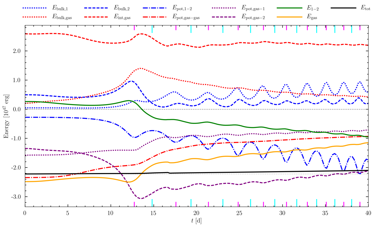
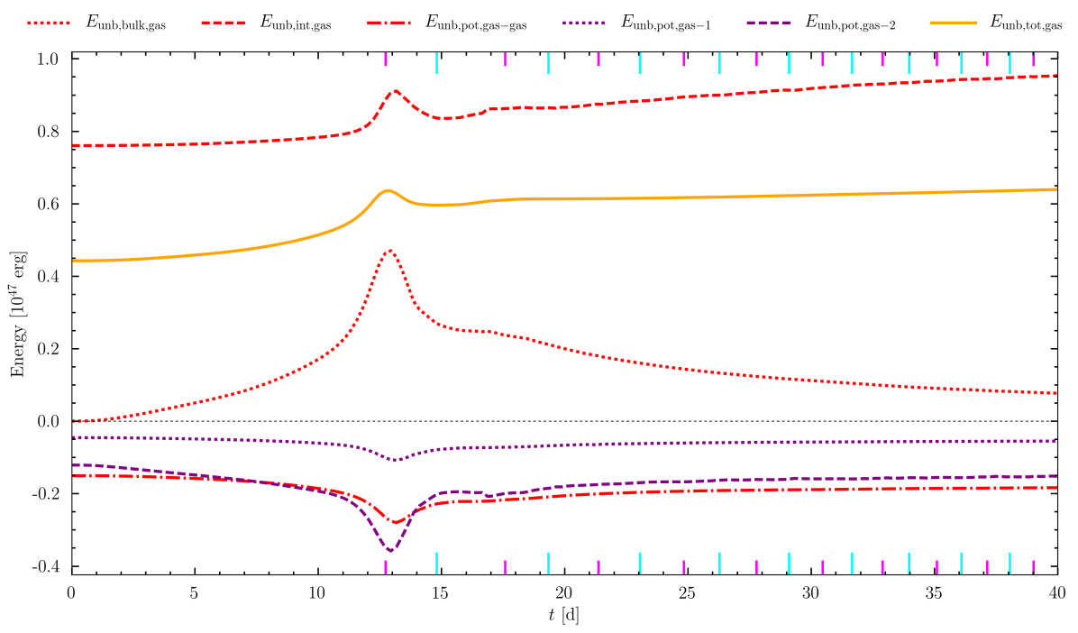
Figure 1: Top: Evolution of the various energy components integrated over the simulation domain (see Tab. 1 for symbol definitions). Those terms involving only particles are plotted in blue, only gas in red, and those involving gas and particles are plotted in mauve. Total energy is shown by a black line, with its initial value plotted as a grey dashed line for reference. Green and orange solid lines show the total particle and gas energies, respectively, with terms involving both particles and gas counting toward the total gas energy. A discontinuity at $t=16.7\,{\rm d}$ is caused by the change in the spline softening length of both particles from $2.4\,\mathrm{R_{\odot}}$ to $1.2\,\mathrm{R_{\odot}}$. The sampling rate of the data plotted is about one frame every $0.23\,{\rm d}$. Times of apastron and periastron passage are shown as long cyan and short magenta tick marks, respectively. Bottom: As in the top panel but now showing the energy of the unbound gas only, where ‘unbound’ is defined as $\mathcal{E}_{\mathrm{gas}}\geq 0$. Note the difference in vertical axis range compared to the top panel.

Table 1: Terms in the energy budget, in units of $10^{47}\,{\rm erg}$, integrated over the simulation domain. Values are shown for the start of the simulation at $t=0$, end of plunge-in at $t=13\,{\rm d}$, and end of the simulation at $t=40\,{\rm d}$. Also shown are the changes in the values between these times. For ease of presentation, expressions involving the gas–particle interactions neglect the modification of the particle potential at distances from the particle less than the spline softening length, but the values quoted were obtained using the full expressions for the potential.

Energy component	Symbol	Expression	$t=0$	$t=13\,{\rm d}$	$t=40\,{\rm d}$	$\mathrm{\Delta}E_{0-13\,{\rm d}}$	$\mathrm{\Delta}E_{13-40\,{\rm d}}$	$\mathrm{\Delta}E_{0-40\,{\rm d}}$
Particle 1 kinetic	$E_{\mathrm{bulk,1}}$	$\tfrac{1}{2}M_{\mathrm{1,c}}v_{\mathrm{1,c}}^{2}$	$0.05$	$0.30$	$0.59$	$0.25$	$0.29$	$0.54$
Particle 2 kinetic	$E_{\mathrm{bulk,2}}$	$\tfrac{1}{2}M_{\mathrm{2}}v_{\mathrm{2}}^{2}$	$0.49$	$0.86$	$0.20$	$0.37$	$-0.66$	$-0.29$
Particle-particle potential	$E_{\mathrm{pot,1-2}}$	$-\mathrm{G}M_{\mathrm{1,c}}M_{\mathrm{2}}/a$	$-0.28$	$-0.96$	$-1.74$	$-0.69$	$-0.78$	$-1.46$
Gas bulk kinetic	$E_{\mathrm{bulk,gas}}$	$\tfrac{1}{2}\int\rho(\bm{x})v_{\mathrm{gas}}^{2}(\bm{x})\mathrm{d}V$	$0.20$	$1.35$	$0.42$	$1.15$	$-0.93$	$0.22$
Gas internal	$E_{\mathrm{int,gas}}$	$\tfrac{3}{2}\int P(\bm{x})\mathrm{d}V$	$2.59$	$2.53$	$2.19$	$-0.06$	$-0.33$	$-0.39$
Gas-gas potential	$E_{\mathrm{pot,gas-gas}}$	$\tfrac{1}{2}\int\Phi_{\mathrm{gas}}(\bm{x})\rho(\bm{x})\mathrm{d}V$	$-2.35$	$-1.90$	$-0.93$	$0.45$	$0.97$	$1.41$
Gas-particle 1 potential	$E_{\mathrm{pot,gas-1}}$	$-\mathrm{G}M_{\mathrm{1,c}}\int(\rho(\bm{x})/|\bm{x}-\bm{x}_{\mathrm{1,c}}|)\mathrm{d}V$	$-1.58$	$-1.40$	$-0.72$	$0.18$	$0.68$	$0.86$
Gas-particle 2 potential	$E_{\mathrm{pot,gas-2}}$	$-\mathrm{G}M_{\mathrm{2}}\int(\rho(\bm{x})/|\bm{x}-\bm{x}_{\mathrm{2}}|)\mathrm{d}V$	$-1.35$	$-2.99$	$-2.12$	$-1.64$	$0.87$	$-0.77$
Particle total	$E_{\mathrm{1-2}}$	$E_{\mathrm{bulk,1}}+E_{\mathrm{bulk,2}}+E_{\mathrm{pot,1-2}}$	$0.26$	$0.20$	$-0.95$	$-0.06$	$-1.15$	$-1.21$
Gas total	$E_{\mathrm{gas}}$	$E_{\mathrm{bulk,gas}}+E_{\mathrm{int,gas}}+\sum_{j}E_{\mathrm{gas-j}}$	$-2.49$	$-2.40$	$-1.15$	$0.08$	$1.25$	$1.33$
Total	$E_{\mathrm{tot}}$	$E_{\mathrm{1-2}}+E_{\mathrm{gas}}$	$-2.22$	$-2.20$	$-2.10$	$0.02$	$0.10$	$0.12$

We write the total energy $E_{\mathrm{tot}}=E_{1-2}+E_{\mathrm{gas}}$. Here $E_{1-2}$ is particle orbital energy and is equal to the sum of particle kinetic energy $E_{\mathrm{bulk,1}}+E_{\mathrm{bulk,2}}$ and mutual potential energy of particles $E_{\mathrm{pot,1-2}}$. Complementally, the binding energy $E_{\mathrm{gas}}$ is defined as the sum of the gas-particle potential energy $E_{\mathrm{pot,gas-1}}+E_{\mathrm{pot,gas-2}}$ plus the gas-only contribution $E_{\mathrm{bulk,gas}}+E_{\mathrm{int,gas}}+E_{\mathrm{pot,gas-gas}}$. Since the binding energy is negative, transferring energy from $E_{1-2}$ to $E_{\mathrm{gas}}$ would make $E_{\mathrm{gas}}$ less negative, and the gas less bound. In what follows, ‘increase’ of energy means toward more positive (or less negative) values, while ‘decrease’ means toward less positive (or more negative) values.

To alleviate confusion from previous literature, we include gas-particle potential energy and gas bulk kinetic energy in $E_{\mathrm{gas}}$, not in $E_{1-2}$. By doing so, we can characterize the problem in terms of transfer between “particle energy” and “gas energy”. The theory is addressed further in Sec. 6 but here we focus on simulation results.

In the top panel of Fig. 1 we show the time-evolution of each energy component integrated over the simulation domain. Apastron and periastron passages are labeled on the time axis by long cyan or short magenta tick marks respectively. Expressions for the various contributions and their values at $t=0$, $t=13\,{\rm d}$ and $t=40\,{\rm d}$, are given in Tab. 1. Time $t=13\,{\rm d}$ is approximately that of first periastron passage and conveniently delineates the transition between the end of the plunge-in phase and the beginning of the slow in-spiral. The inter-particle separation evolves from $a=49.0\,\mathrm{R_{\odot}}$ at $t=0$ to $a=14.1\,\mathrm{R_{\odot}}$ at $t=13\,{\rm d}$ and $a=7.8\,\mathrm{R_{\odot}}$ at $t=40\,{\rm d}$ (Paper I).

A key result from Fig. 1 (top) and Tab. 1 is that the potential energy term $E_{\mathrm{pot,gas-2}}$ is important even when the secondary is situated outside the RG surface at $t=0$ and by the end of plunge-in at $t=13\,{\rm d}$ comprises almost half of the gas potential energy. We note that for a more realistic initial condition for which the initial separation is equal to the Roche limit separation of $\sim 109\,\mathrm{R_{\odot}}$, this term would be less important initially, and the initial energy of the particles and envelope would be less negative by about $0.4\times 10^{47}\,{\rm erg}$ (this is discussed in detail in Sec. 6).

The net energy transferred to $E_{\mathrm{gas}}$ from $t=0$ until $t=13\,{\rm d}$ is negligible even though almost all of the envelope unbinding occurs during this time (Sec. 4). The reason is that although the plunge-in of the secondary violently disrupts and energizes the outer layers of the envelope, it moves the secondary deeper in the envelope and more tightly binds it. The gain in gas kinetic energy is offset by the potential energy becoming more negative, and therefore negligible net exchange between particle energy and gas energy from the start of the simulation up to the end of plunge-in.

Complementally, owing to the continuous and highly variable gravitational force exerted on the particles by the gas, the total particle kinetic energy increases by almost as much as their mutual potential energy decreases between $t=0\,{\rm d}$ and $t=13\,{\rm d}$, resulting in almost zero net change in particle orbital energy.

Subsequently, after $t\approx 15\,{\rm d}$, energy is transferred from particle energy to gas energy at a roughly constant rate as the particles spiral in closer together. We estimate that up to $\sim 0.3\times 10^{47}\,{\rm erg}$ of the intial energy in the particles and envelope is transferred to the ambient gas during the simulation. In the subsections below we expand on these points and discuss each of the curves in the top panel of Fig. 1 in detail.

3.1 Total energy

The total energy is plotted in solid black in Fig. 1 and changes by $5\%$ between $t=0$ and $t=40\,{\rm d}$ (a dotted horizontal grey line shows the initial value for reference). The total energy rises gradually, except for a dip after $t=16.7\,{\rm d}$ when the softening radius around both particles and the smallest resolution element $\delta$, were halved. This discontinuity is expected because reducing the spline softening radius from $r_{\mathrm{soft}}=r_{\mathrm{soft,0}}$ to $r_{\mathrm{soft}}=r_{\mathrm{soft,0}}/2$ immediately strengthens the gravitational force for $r<r_{\mathrm{soft,0}}$. About $16\%$ of the net increase in energy during the simulation is caused by inflow of the ambient medium from the domain boundaries. The remaining error in energy conservation might be caused numerically by the finite time step, which leads to particle orbits that are not completely smooth, or by errors introduced by the multipole Poisson solver. This small variation in the total energy does not affect the conclusions of the present study. We note that our initial RGB star is more bound than the 1D MESA model by about $50\%$ (App. B), and this, along with other details of the setup, imply that our numerical results do not represent detailed observational predictions.

3.2 Particle and gas contributions

The solid green and solid orange lines in the top panel of Fig. 1 show the particle energy $E_{\mathrm{1-2}}$ and gas energy $E_{\mathrm{gas}}$, respectively. The quantity $E_{\mathrm{1-2}}$ is the sum of the quantities shown by the blue curves, namely the kinetic energies of both particles and their mutual potential energy. $E_{\mathrm{1-2}}>0$ at $t=0$ even though the binary system is bound because $E_{\mathrm{1-2}}$ does not include the contribution from $E_{\mathrm{pot,gas-2}}$. $E_{\mathrm{gas}}$ is equal to the sum of the quantities shown by the red and mauve curves pertaining to gas–only and gas–particle energy terms, respectively. The sum $E_{\mathrm{1-2}}+E_{\mathrm{gas}}=E_{\mathrm{tot}}$ is shown in solid black. The green and orange curves show how the orbital energy of the particles is gradually transferred to the gas once the plunge-in phase ends.

To explain the energy evolution in greater detail, we now discuss the relationships between individual energy terms.

3.2.1 Particles

Energy terms pertaining to the particles only (RG core primary, labeled with subscript ‘1’ and hereafter referred to as ‘particle 1,’ and secondary, labeled with subscript ‘2’ and hereafter referred to as ‘particle 2’) are shown in blue. The kinetic energy of particle 1, $E_{\mathrm{bulk,1}}$ (dotted blue), first remains steady and then gradually rises as the inter-particle separation reduces. It oscillates approximately synchronously with the orbit, with maxima in kinetic energy coinciding with periastron passages. The kinetic energy of particle 2, $E_{\mathrm{bulk,2}}$ (dashed blue), first increases during the plunge-in phase from $t=8$ and $t=13\,{\rm d}$. This $E_{\mathrm{bulk,2}}$ then decreases as the secondary migrates from having orbited the larger RG (core+envelope) mass to orbiting primarily only the smaller mass of particle 1. Following this decrease, $E_{\mathrm{bulk,2}}$ then rises less rapidly than $E_{\mathrm{bulk,1}}$, as there is continued competition between reduced particle separation and reduced gas mass interior to the orbit. Naturally, $E_{\mathrm{bulk,2}}$ oscillates in phase with $E_{\mathrm{bulk,1}}$.

The potential energy of particles $E_{\mathrm{pot,1-2}}$ (which excludes that from gas–particle gravitational forces) is shown in dash-dotted blue, and its mean value over an orbit period reduces by $1.7\times 10^{47}\,{\rm erg}$ between $t=0$ and $t=40\,{\rm d}$. $E_{\mathrm{pot,1-2}}$ steadily decreases at $t=40\,{\rm d}$, even as the rate of change of the mean inter-particle separation $\dot{\overline{a}}(<0)$ (where bar denotes mean) reduces in magnitude (Paper I) so that $\ddot{\overline{a}}>0$. This behaviour is expected from the $1/a$ Newtonian potential; for a circular orbit this gives $\dot{E}_{\mathrm{pot,1-2}}\propto\dot{a}/a^{2}$ so the decrease in $|\dot{a}|$ competes with the reduction in $a$. Whether $\ddot{E}_{\mathrm{pot,1-2}}$ is positive or negative depends on the details of orbital evolution.

3.2.2 Gas

Energy terms pertaining to gas only are shown in red in Fig. 1. The total bulk kinetic energy of gas $E_{\mathrm{bulk,gas}}$ (dotted red) rises during plunge-in as envelope material is propelled outward and then gradually reduces as gravity and shocks decelerate the envelope. The dashed red curve shows the internal energy of the gas $E_{\mathrm{int,gas}}$, of which about $0.8\times 10^{47}\,{\rm erg}$ comes from the ambient medium. The latter has a pressure of $1\times 10^{5}\,{\rm dyn\,cm^{-2}}$ and fills the simulation domain. The ambient medium hardly contributes to $E_{\mathrm{bulk,gas}}$ however. $E_{\mathrm{int,gas}}$ is initially fairly steady, but then incurs modest variations from gas expansion and compression. Both $E_{\mathrm{int,gas}}$ and $E_{\mathrm{bulk,gas}}$ show small-amplitude oscillations with maxima approximately coinciding with periastron passages.

Each close encounter of the particles dredges up material in dual spiral wakes. During plunge-in, the gas acquires mostly bulk kinetic energy, but also significant internal energy, as expected from the observed spiral shocks. The subsequent slow decrease of $E_{\mathrm{bulk,gas}}$ is accompanied by an increase in potential energy from gas self-gravity $E_{\mathrm{pot,gas-gas}}$ (dash-dotted red). Of the total $E_{\mathrm{pot,gas-gas}}$, the gravitational interaction between the ambient medium and envelope and that of the ambient medium with itself respectively contribute the relatively small amounts of $0.2\times 10^{47}\,{\rm erg}$ and $0.1\times 10^{47}\,{\rm erg}$. Between $t=0$ and $t=40\,{\rm d}$, substantial work ($1.4\times 10^{47}\,{\rm erg}$) is done expanding the envelope against its own gravity. In principle, unbinding the gas from the particles does not require the gas to become unbound from itself, but much of the kinetic energy acquired by the envelope in the simulations is drained into expansion against its own self-gravity.

3.2.3 Gas-particles interaction

The mauve curves in Fig. 1 show the potential energy terms accounting for the gas–particle 1 gravitational force $E_{\mathrm{pot,gas-1}}$ (dotted mauve) and gas–particle 2 gravitational force $E_{\mathrm{pot,gas-2}}$ (dashed mauve). These terms must be included in assessing the extent to which the envelope is bound. The ambient medium contributes negligibly to them ($<0.2\times 10^{47}\,{\rm erg}$ total).

Initially the inner layers of the RG are hardly affected by interaction with the secondary, and so $E_{\mathrm{pot,gas-1}}$ varies slowly until the plunge-in, when the inner envelope is strongly disrupted. After the end of the plunge-in at $t=13\,{\rm d}$, $E_{\mathrm{pot,gas-1}}$ increases with time as work is done to expand the envelope against the gravitational force from particle 1, situated roughly at its centre.

The gravitational interaction between gas and particle 2 (dashed mauve) is a bit more subtle and not fully accounted for in previous analyses using the CE energy formalism. Even at $t=0$, $E_{\mathrm{pot,gas-2}}$ is important, being almost equal to $E_{\mathrm{pot,gas-1}}$ because particle 1 is closer to the bulk of the gas even though particle 2 is more massive. However, as particle 2 plunges toward the envelope centre, $E_{\mathrm{pot,gas-2}}$ increases in magnitude by $1.6\times 10^{47}\,{\rm erg}$ and by $t=13\,{\rm d}$ becomes the most important contribution to the gas potential energy. From $t=0$ until the end of plunge-in, $E_{\mathrm{gas}}$ gains only $0.1\times 10^{47}\,{\rm erg}$, or about $3\%$. This highlights that the liberation of orbital energy as particle 2 plunges in does not come “for free” because when $M_{\mathrm{2}}$ arrives close to the envelope centre, the envelope is bound inside a much deeper potential well. During plunge-in, the energy liberated by $E_{\mathrm{pot,gas-2}}$ becoming more negative is transferred to the bulk kinetic energy of gas. Part of this kinetic energy does work to expand the envelope against gravity, as evidenced by increases in the gas-particle 1 and gas-gas potential energies.

From $t=13\,{\rm d}$ to $t=40\,{\rm d}$, the envelope then expands to become less bound at the expense of the gas kinetic energy (dotted red) and particle–particle potential energy (dash-dotted blue) and significant work is expended on moving gas outward against self-gravity and the gravitational forces of particle 2 and particle 1.

4 Partial envelope unbinding

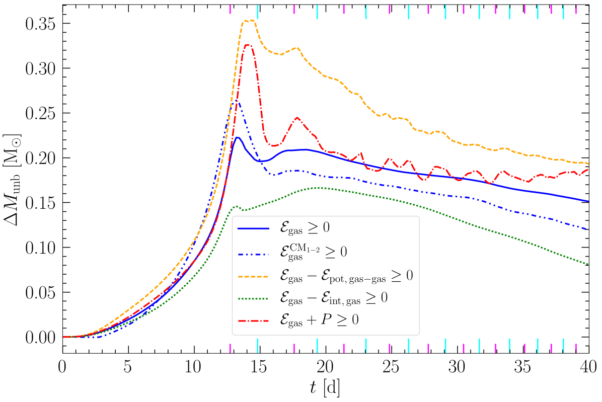
Figure 2: Change in unbound mass of the envelope with time according to the fiducial definition of ‘unbound,’ $\mathcal{E}\geq 0$ (solid blue), as well as various alternative definitions labeled in the legend (see Sec. 4).

We delineate gas as ‘unbound’ if its total energy density, $\mathcal{E}_{\mathrm{gas}}=\mathrm{\delta}E_{\mathrm{gas}}/\mathrm{\delta}V\geq 0$, where $\mathcal{E}_{\mathrm{gas}}$ equals the sum of bulk kinetic, internal and potential (due to self-gravity and interactions with both particles) energy densities.

As we explain below, virtually all of the unbinding of gas occurs between the start of the simulation and end of the plunge-in phase. As will become apparent in Sec. 4.2, this happens in spite of the negligible total energy transfer between particle orbital energy and gas binding energy (Sec. 3), but can be explained by recognizing that the nature and relative importance of energy exchange between various forms depends strongly on position.

4.1 Unbound mass

In Fig. 2 we plot the change in the unbound mass (defined by $\mathcal{E}_{\mathrm{gas}}\geq 0$) as a function of time (solid blue), not including the unbound ambient gas that inflows through the domain boundaries. Note that most of the ambient medium is already unbound at $t=0$ (about $1.7\,\mathrm{M_{\odot}}$). Only a small amount of ambient mass is bound at $t=0$ ($<0.04\,\mathrm{M_{\odot}}$), and while some of this bound mass may become unbound during the course of the simulation, its contribution to Fig. 2 would be negligible. In principle there could also be a small negative contribution from unbound ambient mass becoming bound, but data from 2D slices suggests that unbound ambient material, located at a distance $\gtrsim 200\,\mathrm{R_{\odot}}$ from particle 1, generally remains unbound. Therefore, the change in unbound mass $\mathrm{\Delta}M_{\mathrm{unb}}$ plotted in Fig. 2 corresponds quite closely to the unbinding of bound envelope material.

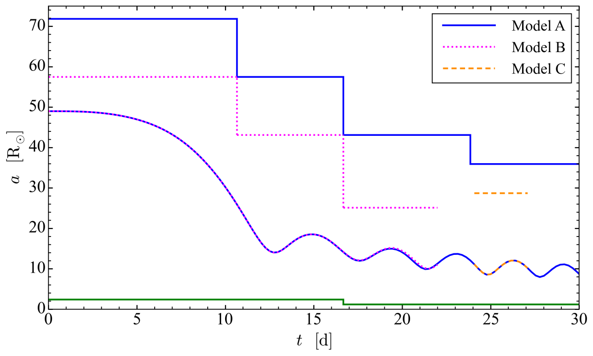
Figure 9: Orbital separation $a$ between particles 1 and 2, now plotted along with the radius $r_{\mathrm{ref}}$ of the spherical volume refined at the highest level (jagged line with colour the same colour as the separation curve for that run). Plotted are the fiducial run, Model A (solid blue), as well as Models B (dotted magenta) and C (dashed orange), which both have smaller refinement radius $r_{\mathrm{ref}}$ than Model A. The softening radius $r_{\mathrm{soft}}$ (same for all runs) is also shown, for reference (solid green).

The unbound mass increases from the start of the simulation until the end of plunge-in, then reduces slightly, recovers, levels off at $t\approx 17\,{\rm d}$, and then decreases steadily after $t\approx 19\,{\rm d}$. The steady decrease is caused by energy transferred from the envelope to the ambient medium. We estimate the total energy transfer in Sec. 4.3. As the ambient material has fairly large density and pressure in our simulation, this decrease is not seen in most other simulations. In nature, a circumbinary torus formed during the Roche-lobe overflow (RLOF) phase would be present and likely produce a similar effect. A peak in the unbound mass near the first periastron and a subsequent levelling off is also seen in the phantom simulation of Iaconi et al. (2017) (see their Fig. 9, top panel for results from the run with the most comparable setup to ours; see also Iaconi et al. 2018), and other CEE simulations (Sandquist et al., 2000; Passy et al., 2012; Nandez et al., 2014). However, in Ricker & Taam (2012), unbinding peaks near the first periastron but continues for several orbits until the end of the simulation. In Sandquist et al. (1998), unbinding occurs around the first periastron, stops, and then restarts much later in the evolution (visible as a relative drop in the bound mass as compared to the mass that leaves the grid, and most significant for their simulations 4 and 5).

By $t=13\,{\rm d}$ the total change in unbound mass is given by $\mathrm{\Delta}M_{\mathrm{unb}}\approx 0.22\,\mathrm{M_{\odot}}$ or about $14\%$ of the envelope mass, and this reduces to $0.21\,\mathrm{M_{\odot}}$ or $13\%$ of the envelope mass between $t\approx 17\,{\rm d}$ and $t\approx 19\,{\rm d}$. This is comparable to the fraction of $13\%$ obtained by Iaconi et al. (2017). Using the moving mesh code arepo with initial conditions very close to ours, Ohlmann et al. (2016) obtained a value of $8\%$ by the end of their simulation, and found that most of this was ejected during the first $40\,{\rm d}$. The difference between their value and ours is likely caused by the slight differences in initial conditions (see App. A for a detailed comparison, and a discussion of differences in the initial conditions). We note that our initial RGB primary is significantly more strongly bound than the MESA star from which it is modeled (see App. B), and this alone would be expected to lead to an underestimate of the amount of unbinding. However, as with all CEE simulations to date, other physics, such as convection and radiation transport, are also absent, and initial conditions are not fully realistic. We reiterate that the main goal, as stated in the introduction, is not to predict observations precisely, but rather to understand and account for energy transfer and envelope unbinding in the simulation, given the choices of the setup.

Although the gas energy $E_{\mathrm{gas}}$ hardly changes between $t=0$ and the end of plunge-in at $t\approx 13\,{\rm d}$ (and likewise for $E_{1-2}$ since the two are complementary; see Sec. 3), this is when most of the envelope unbinding occurs. Some of the gas gains energy to become less bound, while the remainder loses energy to become more bound and the net change is nearly zero. This happens as the secondary plunges toward the bulk of material at the centre, strengthening its overall pull on the envelope, but also imparting an impulse to the gas it encounters locally. To understand this in more detail, we discuss the spatial variation of the energy density in Sec. 4.2.

The other lines in Fig. 2 represent changes in unbound mass using alternative definitions of ‘unbound’. More liberal definitions plotted are $\mathcal{E}_{\mathrm{gas}}-\mathcal{E}_{\mathrm{pot,gas-gas}}\geq 0$ (exclusion of self-gravity; orange dashed), $\mathcal{E}_{\mathrm{gas}}+P\geq 0$ (replacement of internal energy density with enthalpy density; red dashed-dotted), and $\mathcal{E}_{\mathrm{gas}}^{\mathrm{CM_{1-2}}}\geq 0$, where the left-hand-side is the gas energy density in the frame of the particles’ centre of mass (blue dashed-double-dotted; we motivate this choice in Sec. 5). We also plot $\mathcal{E}-\mathcal{E}_{\mathrm{int,gas}}\geq 0$ (exclusion of the internal energy density; green dotted) for comparison. For each curve, the unbound mass at $t=0$, located in the ambient medium, is subtracted from the total unbound mass, as well as any unbound mass that has entered through the domain boundaries.

Ivanova & Nandez (2016) previously argued that energy deposition occurs only outside the orbit of the particles. Although the gas between the particles is not undisturbed as seen in 2D slices of density or energy (Sec. 4.2 and Paper I), the effect on the gas outside the orbit is likely stronger than inside it. In calculating the unbound mass fraction it is then an interesting alternative to exclude the mass of gas within a sphere of radius $a(t)$ centred on particle 1. About $23\%$ of the envelope mass resides within a distance $a$ from particle 1 at $t=13\,{\rm d}$, dropping to $3\%$ at $t=40\,{\rm d}$. At both times, most all of this interior mass is bound. Therefore, the change in the unbound mass for the ‘exterior’ envelope is basically unchanged from the values we calculated for the whole envelope (Fig. 2). The total envelope mass is $1.6\,\mathrm{M_{\odot}}$ and at the end of plunge-in at $t=13\,{\rm d}$, $18\%$ of the envelope mass exterior to the orbit is unbound, compared with $14\%$ of the whole envelope.

4.2 Spatial analysis

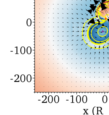
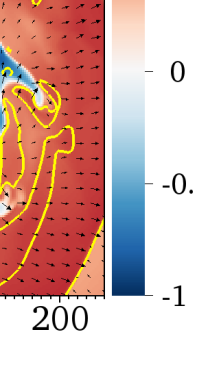
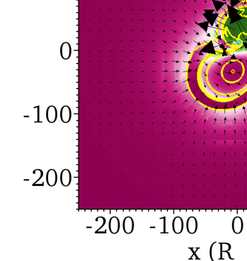
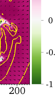
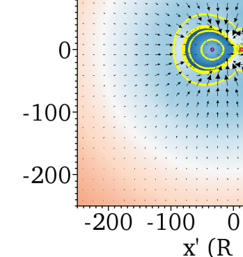
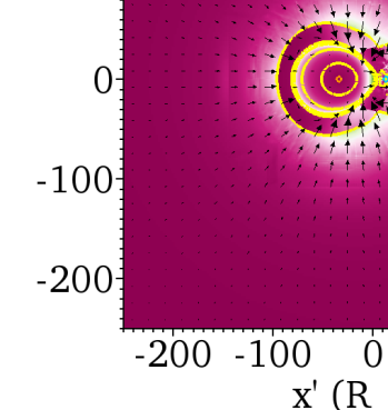
Figure 3: Top row: Snapshots of the quantity $\mathcal{E}_{\mathrm{gas}}/\max(\mathcal{E}_{\mathrm{bulk,gas}}+\mathcal{E}_{\mathrm{int,gas}},-\mathcal{E}_{\mathrm{pot,gas}})$, where $\mathcal{E}_{\mathrm{pot,gas}}=\mathcal{E}_{\mathrm{pot,gas-1}}+\mathcal{E}_{\mathrm{pot,gas-2}}+\mathcal{E}_{\mathrm{pot,gas-gas}}$, in the orbital plane at $t=5$, $10$, $20$ and $30\,{\rm d}$. This is the gas energy density, normalized to the magnitude of the gas kinetic energy density (internal + bulk) or the total gas potential energy density, whichever is greater. A value of $1$ corresponds to a maximally unbound system, while a value of $-1$ corresponds to a maximally bound system, for our standard definition of ‘unbound’: $\mathcal{E}_{\mathrm{gas}}\geq 0$. At $t=0$, both particles are situated on the $x$-axis with particle 2 (circular red contour near centre) located to the right of particle 1 (circular mauve contour near centre), and the orbit is anti-clockwise. Yellow contours show the density from $\rho=10^{-4}\,{\rm g\,cm^{-3}}$ downward in logarithmic intervals of 1 dex. Vectors show the component of the velocity parallel to the orbital plane (representing the points located at the ends of the arrow tails). The frame of reference is that of the simulation, and each plot is centred on the particle centre of mass. Second row from top: As for the top row but now showing the quantity $(\mathcal{E}_{\mathrm{int,gas}}-\mathcal{E}_{\mathrm{bulk,gas}})/\max(\mathcal{E}_{\mathrm{int,gas}},\mathcal{E}_{\mathrm{bulk,gas}})$. This compares the internal and bulk kinetic energy densities. Magenta means internal energy dominates (between the two forms), green means bulk kinetic energy dominates, and white means they are approximately equal. Softening spheres are now represented by orange and cyan contours for particles 1 and 2, respectively. Second row from bottom: As top row but now for the $x^{\prime}$-$z$ plane, which is orthogonal to the orbital plane and intersects both particles. Bottom row: As second row from top but now for the $x^{\prime}$-$z$ plane.

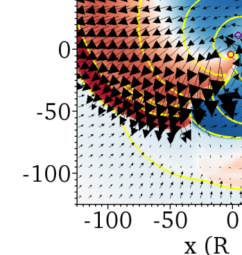
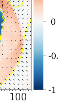
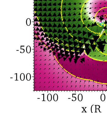
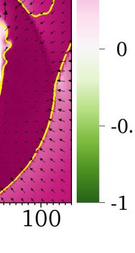
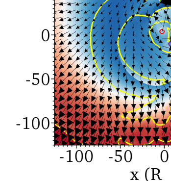
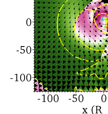
Figure 4: Similar to the top two rows of Fig. 3 but zoomed in and showing eight snapshots equally spaced in time (by about $0.9\,{\rm d}$) between $t=12.0\,{\rm d}$ and $t=18.5\,{\rm d}$. Particles complete only a fraction of an orbital revolution between successive snapshots. In the top row, showing $t=12.0\,{\rm d}$ to $t=14.8\,{\rm d}$, the most recently energized unbound material (red, near particle 2) becomes bound (blue) when it loses kinetic energy as it collides with the bulk of the envelope material. In the second-from-bottom row, showing $t=15.7\,{\rm d}$ to $t=18.5\,{\rm d}$, some of the bound material in the spiral wake of particle 2 becomes unbound (above centre) as it moves into a lower density region.

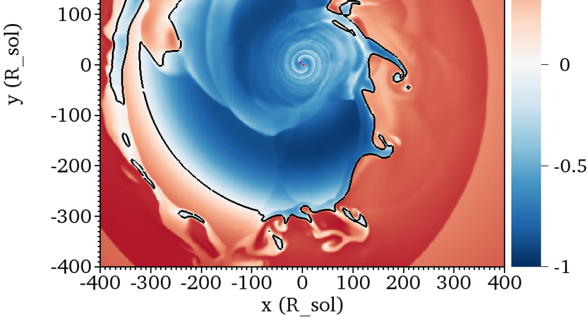
Figure 5: caption The normalized gas energy $\mathcal{E}_{\mathrm{gas,norm}}$ with blue (red) showing bound (unbound) gas at $t=40\,{\rm d}$, with contours delineating the value zero. Recently formed islands of bound gas are seen near the envelope-ambient interface, showing how unbound envelope gas can become bound as it transfers energy to the ambient medium. The CM of the particles is at (0,0) and the primary and secondary particle softening spheres are represented by mauve and red contours, respectively (near centre, barely visible due to the scale of the plot).

To interpret Fig. 2 and the partial unbinding of the envelope, we now explore the time-dependent spatial distribution of energy. We define a normalized energy density $\mathcal{E}_{\mathrm{gas,norm}}=\mathcal{E}_{\mathrm{gas}}/\max(\mathcal{E}_{\mathrm{bulk,gas}}+\mathcal{E}_{\mathrm{int,gas}},\;-\mathcal{E}_{\mathrm{pot,gas}})$ (where $\mathcal{E}_{\mathrm{pot,gas}}=\mathcal{E}_{\mathrm{pot,gas-1}}+\mathcal{E}_{\mathrm{pot,gas-2}}+\mathcal{E}_{\mathrm{pot,gas-gas}}$) and plot snapshots of $\mathcal{E}_{\mathrm{gas,norm}}$ in the orbital plane in the top row of Fig. 3 for $t=5$, $10$, $20$ and $30\,{\rm d}$. The quantity $\mathcal{E}_{\mathrm{gas,norm}}$ is the local gas energy density normalized by either the magnitude of the local gas kinetic energy density (bulk and internal) or the magnitude of the local gas potential energy density, whichever is greater. For our fiducial definition of unbound, $\mathcal{E}_{\mathrm{gas}}\geq 0$, blue corresponds to bound material while red corresponds to unbound material, and $-1$ ($1$) means maximally bound (unbound). Much of the ambient material is initially unbound due to its large internal energy density and large distance from the central mass concentration. Contours show the gas density while the component of the velocity in the orbital plane is shown with arrows.

The second row of Fig. 3 shows $(\mathcal{E}_{\mathrm{int,gas}}-\mathcal{E}_{\mathrm{bulk,gas}})/\max(\mathcal{E}_{\mathrm{int,gas}},\mathcal{E}_{\mathrm{bulk,gas}})$. This is the difference between the local internal energy density and the local bulk kinetic energy density, normalized by whichever of the two is largest. Magenta (green) represents gas for which $\mathcal{E}_{\mathrm{int,gas}}$ is larger (smaller) than $\mathcal{E}_{\mathrm{bulk,gas}}$ and the limits are $1$ (all internal) and $-1$ (all bulk kinetic). These plots correspond closely with similar plots for Mach number (not shown); magenta (green) regions correspond to subsonic (supersonic) gas. The third and fourth rows of Fig. 3 show the same quantities as the top two rows, but in a slice through the plane orthogonal to the orbital plane that intersects the particles (the $x^{\prime}$-$z$ plane). Fig. 4 shows a sequence of eight snapshots for each quantity, spaced by $\sim 0.9\,{\rm d}$, between $t=12.0\,{\rm d}$ and $18.5\,{\rm d}$, now zoomed in by a factor of two compared with those of Fig. 3.

During the plunge-in, material is torn away from the envelope by the secondary, forming a tidal bulge that wraps around in a spiral morphology, trailing the secondary in its orbit (density contours). Gas closest to particle 2 in this spiral wake moves supersonically in a direction in between radially outward and tangential to the path of particle 2. The wake contains highly supersonic unbound gas extending from particle 2 (red and green in the topmost and second-from-top rows, respectively), surrounding a bound region (blue and magenta/yellow) trailing particle 2. Where the spiral wake encounters the low density ambient medium, a spiral shock forms. This does not greatly effect the motion of the outward moving unbound gas (see Sec. 4.3) which slows as it climbs out of the potential well.

At $t\approx 11\,{\rm d}$, after roughly the first half-orbital revolution, newly unbound material near particle 2, followed by particle 2 itself and the dense bulge trailing it, violently collide with dense gas in the bulk of the relatively undisturbed RG envelope. This occurs as the inter-particle separation shrinks rapidly from dynamical friction while the secondary, with its near-side tidal bulge in tow, catches up to the tidal bulge of the RG on the far side of the RG from the secondary that lags the particles in their orbit.

From the collision, an almost radial spiral shock forms near the secondary that connects to the primarily azimuthal shock farther out. This can be seen in the top two rows of Fig. 4, showing the evolution of $\mathcal{E}_{\mathrm{gas,norm}}$ and $(\mathcal{E}_{\mathrm{int,gas}}-\mathcal{E}_{\mathrm{bulk,gas}})/\max(\mathcal{E}_{\mathrm{int,gas}},\mathcal{E}_{\mathrm{bulk,gas}})$ between $12.0\,{\rm d}$ and $14.8\,{\rm d}$. Note that the velocity of the gas immediately left of the shock (shown by vector arrows) decreases as the shock forms. The shock structure widens in time as more gas gets shocked. Correspondingly, bulk kinetic energy is converted to internal energy at $t\approx 13\,{\rm d}$, consistent with the quantitative evolution of the contributions to the global energy budget shown in Fig. 1.

However, the total energy density $\mathcal{E}_{\mathrm{gas}}$ in the central part of the spiral wake near the secondary decreases between $t\approx 13\,{\rm d}$ and $t\approx 15\,{\rm d}$, causing unbound material to become bound once again. This is visible in the top part of Fig. 4, where red material near the secondary becomes blue. We can see that at $t\approx 13\,{\rm d}$ (termination of plunge-in), the unbound part of the wake “detaches” from the secondary because the secondary no longer supplies enough energy to unbind the material in its immediate surroundings. This material lies deep in the potential well and is surrounded by dense overlying layers that impede its outward motion. The part of the spiral wake that transitions from unbound to bound between $t\approx 13\,{\rm d}$ and $t\approx 15\,{\rm d}$ explains the peak and subsequent dip in total unbound mass in Fig. 2 at $t\approx 13\,{\rm d}$ (blue solid curve).

The subsequent rise in the unbound mass starting at $t\approx 15\,{\rm d}$ and lasting for a few days can be explained with reference to the bottom row of Fig. 4, which shows the time frame $t=15.7\,{\rm d}$ to $t=18.5\,{\rm d}$. At this time (about 1.5 orbital revolutions after the start of the simulation) the shocked spiral structure trailing the secondary moves at an angle $<90^{\circ}$ with respect to the far-side tidal bulge gas, and their relative velocity is much smaller than when they first collided. The inertia of the dense spiral wake and the negative pressure gradient (nearly aligned to the density gradient) allow the wake to accelerate up to a nearly constant speed toward larger $y$. This happens in spite of the work done by gravity so the overall energy density of the wake increases.

This process repeats during the next orbital revolution, resulting in a third layer of unbound gas that can be seen as the innermost strip of red on the upper-left of the rightmost panel in the top row of Fig. 3 at $t=30\,{\rm d}$. By this time, a separate spiral wake trails behind particle 1, but this wake does not gain enough energy as it moves outward to become unbound. In subsequent orbital revolutions, a smaller amount of material transitions from bound to unbound, now toward positive $x$; an example is visible in the same panel at $t=30\,{\rm d}$ (right of centre in the plot). In this snapshot, Rayleigh-Taylor (RT) instability-produced “fingers” are visible at large distances from the centre. Such features are formed as the outward-moving interface between inner dense gas and outer diffuse gas decelerates.

After $t\approx 19\,{\rm d}$, pockets of gas can be seen to transition from unbound to bound near the edge of the expanding envelope. This is most obvious late in the simulation. In Fig. 5 we show a snapshot at $t=40\,{\rm d}$. In addition to the RT fingers of bound material mentioned above, recently formed isolated blue “islands” of bound material are visible.

4.3 Efficiency of partial envelope removal

Since unbound material will never have exactly zero energy density, there is always an efficiency associated with the energy transfer process. To get an idea about how much energy is “wasted” by increasing the energy density of already unbound material, we plot various energy components with time for gas that is unbound in the bottom panel of Fig. 1. From the orange line, we see that during the simulation a net amount of about $0.2\times 10^{47}\,{\rm erg}$ of energy is gained by the unbound gas. As the change in gas energy during the simulation is $1.3\times 10^{47}\,{\rm erg}$, the fraction that ends up in already unbound gas is about $15\%$. This gives us an estimate of how much of the particle energy is wasted.

How does the energy transfer to unbound material take place and what happens subsequently? We see from the bottom panel of Fig. 1 that most of the increase in energy of the unbound material occurs in the first $13\,{\rm d}$. This is consistent with the change in the unbound mass $\mathrm{\Delta}M_{\mathrm{unb}}$ also peaking at $t\approx 13\,{\rm d}$. The energy transferred is mainly in the form of kinetic energy, as material is launched outward during plunge-in. Subsequently, the unbound gas, whose mass remains almost constant after $t=13\,{\rm d}$, sees much of its bulk kinetic energy get converted to internal energy and potential energy.

There is another way in which energy transfer to the envelope is inefficient. To expand, the envelope must displace ambient material, which has significant pressure and mass in our simulation. Work must be done by the envelope against thermal pressure of the ambient material, ram pressure as the envelope expands into ambient gas, and also to displace ambient material against gravity. These terms can respectively be estimated as $\sim(4\pi/3)P_{\mathrm{amb}}r_{\mathrm{f}}^{3}$, $\sim(4\pi/3)\rho_{\mathrm{amb}}v_{r}^{2}r_{\mathrm{f}}^{3}$ and $\sim(4\pi/3)\mathrm{G}r_{\mathrm{f}}^{2}(M_{\mathrm{1}}+M_{\mathrm{2}})\rho_{\mathrm{amb}}$, where $P_{\mathrm{amb}}=1\times 10^{5}\,{\rm dyn\,cm^{-2}}$ is the ambient pressure, $\rho_{\mathrm{amb}}=7\times 10^{-9}\,{\rm g\,cm^{-3}}$ is the ambient density, $M_{\mathrm{1}}=2\,\mathrm{M_{\odot}}$ is the primary mass, $M_{\mathrm{2}}=1\,\mathrm{M_{\odot}}$ is the secondary mass, $r_{\mathrm{f}}\sim 3\times 10^{13}\,{\rm cm}$ is the radius of the envelope at $t=40\,{\rm d}$, and $v_{r}\sim 40\,{\rm km\,s^{-1}}$ is a typical speed at which the envelope expands into the surroundings. With these expressions we obtain $\sim 0.1\times 10^{47}\,{\rm erg}$ for each work term. Thus, $\sim 0.3\times 10^{47}\,{\rm erg}$ may have been transferred from the envelope to the ambient medium during the course of the simulation. This is a small amount compared to the total envelope energy, but indicates that the expansion of the envelope would have been slightly faster within a less dense or lower pressure ambient medium. It also explains the decrease in unbound mass after $t\approx 19\,{\rm d}$. A circumbinary torus is likely to remain from the RLOF stage preceding CEE, and this material would shape the envelope and redirect its expansion (Metzger & Pejcha, 2017; MacLeod et al., 2018a; Reichardt et al., 2018).

4.4 Timescale for ejecting the envelope and final separation

The average rate of energy transfer from the particles to the gas is approximately constant at the end of the simulation, and equal to about $0.03\times 10^{47}\,{\rm erg}\,{\rm d}^{-1}$ (final average slope of orange curve of top panel of Fig. 1). Of this transfer rate, about $0.001\times 10^{47}\,{\rm erg}\,{\rm d}^{-1}$, a negligible fraction, is being transferred from the particles to gas that is already unbound (final slope of orange curve of bottom panel of Fig. 1). Thus, although the envelope continues to gain energy at a relatively high rate, this energy is being gained by material that is still bound by the end of the simulation. Assuming that this energy transfer rate of $0.03\times 10^{47}\,{\rm erg}\,{\rm d}^{-1}$ remains constant, one can estimate how long it would take for the gas to attain zero total energy, and we find it would take an additional $38\,{\rm d}$. However, this calculation uses the total gas energy, which includes the energy of the ambient medium, equal to $E_{\mathrm{amb}}\sim 0.5\times 10^{47}\,{\rm erg}$. Thus, to obtain a more accurate estimate, we subtract this ambient energy from the value of $E_{\mathrm{gas}}$ at $t=40\,{\rm d}$ given in Tab. 1, which gives an envelope gas energy of $E_{\mathrm{e}}\sim-1.65\times 10^{47}\,{\rm erg}$. Then the additional time needed for the envelope to attain $E_{\mathrm{gas}}=0$ would be about $55\,{\rm d}$ after the end of the simulation at $t=40\,{\rm d}$.

Now, from Sec. 4.3 we know that not all of the liberated particle orbital energy will be transferred to bound material, and that this leads to an efficiency factor $\epsilon$, found to be about $85\%$ in the first $40\,{\rm d}$ (that is, $15\%$ of the energy gets wasted). Assuming an efficiency of $\epsilon=0.85$ for the remainder of the evolution, the time calculated above must be divided by $\epsilon$, giving $\sim 65\,{\rm d}$. As the system continues to evolve, less and less gas would remain bound, so we would expect that more of the released orbital energy would go into unbound gas, resulting in reduced efficiency. With an efficiency of only $10\%$, the released orbital energy would have to be about $16.5\times 10^{47}\,{\rm erg}$, and the timescale for ejecting the envelope would be $\sim 550\,{\rm d}$, or about $1.5\,{\rm yr}$, which is small enough to be consistent with observations of post-CE binary systems, for which the envelope has already been ejected. In Ohlmann et al. (2016), the orbital energy decay rate of the particles decreases to become much smaller by the end of their simulation at $t\sim 130\,{\rm d}$ than at $t=40\,{\rm d}$. The assumption that this decay rate remains constant is therefore probably too optimistic.

The orbital energy of the particles at $t=40\,{\rm d}$ is about $E_{1-2}(40\,{\rm d})=-0.95\times 10^{47}\,{\rm erg}$ (Tab. 1). Then, equating the gas energy with the difference in particle energy between $t=40\,{\rm d}$ and envelope ejection, multiplied by the efficiency $\epsilon$, we derive the following expression for the final separation:

$$a_{\mathrm{f}}\sim\frac{\mathrm{G}M_{\mathrm{1,c}}M_{\mathrm{2}}}{2}\left(\frac{E_{\mathrm{amb}}-E_{\mathrm{gas}}(40\,{\rm d})}{\epsilon}-E_{1-2}(40\,{\rm d})\right)^{-1}.$$ (1)

This estimate is independent of the rate of energy transfer (and foreshadows our discussion of the CE EF in Sec. 6). Putting $\epsilon=1$ gives the upper limit $a_{\mathrm{f}}\sim 2.9\,\mathrm{R_{\odot}}$, while for $\epsilon=0.85$ we obtain $a_{\mathrm{f}}\sim 2.6\,\mathrm{R_{\odot}}$ and for $\epsilon=0.1$ we obtain $a_{\mathrm{f}}\sim 0.4\,\mathrm{R_{\odot}}$.

5 Particle centre of mass motion and planetary nebula–central star offsets

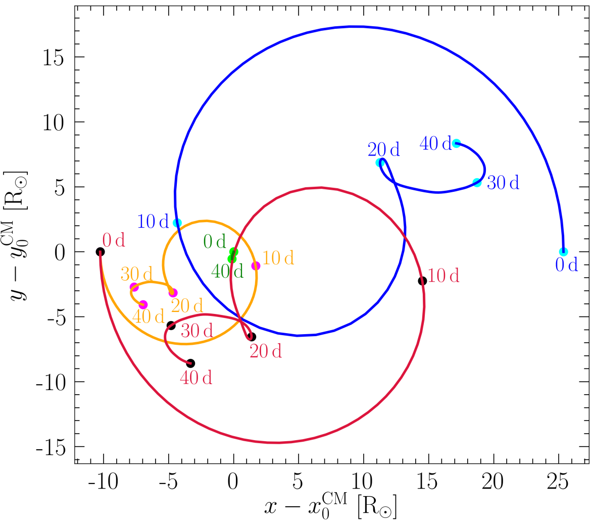
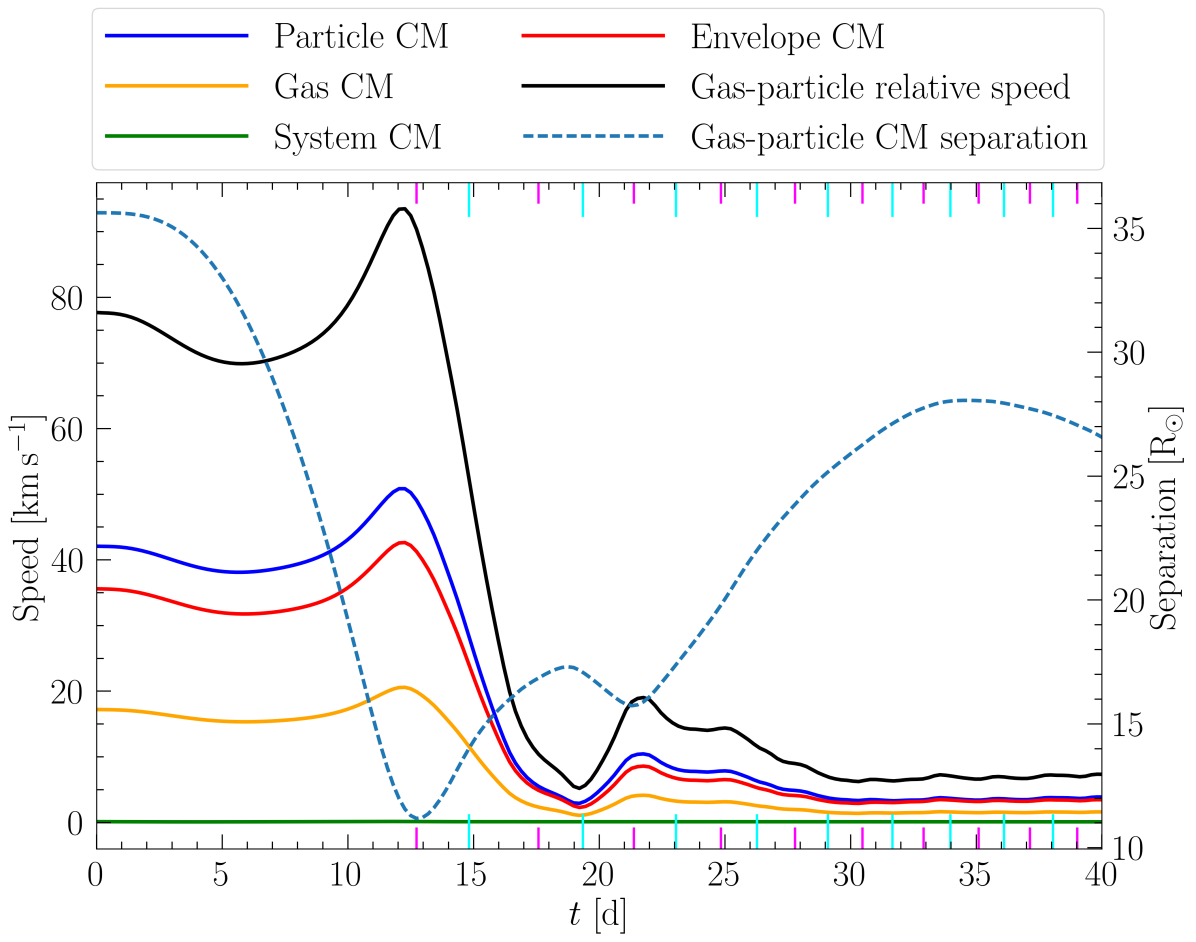
Figure 6: Top: Motion in orbital plane of the particle CM (blue), gas CM (orange), envelope CM (red) and net system CM (green). The system CM moves slowly and gradually downward in the plot during the course of the simulation. Bottom: Evolution of the speed relative to the reference frame in which the simulation is carried out, for the particle CM (blue), gas CM (orange), envelope CM (red) and net system CM (green). The relative speed between the envelope CM and particle CM is shown in black. Also plotted, using the right vertical axis, is the separation between the envelope CM and particle CM (dashed).

The asymmetry of the gas distribution in the orbital plane rapidly evolves, moving the particle and gas centres of mass (CM) oppositely in the simulation frame, while nearly conserving linear momentum (see also Sandquist et al., 1998; Ohlmann et al., 2016). The top panel of Fig. 6, shows the paths in the orbital plane traced by the particle CM (blue), gas CM (accounting for both envelope and ambient gas, orange), envelope CM (red), and system CM (green). The position and motion of the envelope CM are obtained by assuming that the CM of ambient gas remains fixed during the simulation. The system CM position remains relatively fixed with small speed ($<0.2\,{\rm km\,s^{-1}}$); deviations in its position are caused by small errors in linear momentum conservation.

The bottom panel of Fig. 6 shows the speed of the particle CM versus time in blue, that of the gas CM in orange, that of the envelope CM in red, and that of the system CM in green, as well as the relative speed between envelope CM and particle CM in black. Until the end of the plunge-in phase at $t\approx 13\,{\rm d}$, the relative speed between the envelope CM and particle CM is $70$-$94\,{\rm km\,s^{-1}}$, and the final relative speed is $7$ to $8\,{\rm km\,s^{-1}}$. Sandquist et al. (1998) found the speed of the particle CM relative to the system CM frame at the late stages of CEE to be $3\,{\rm km\,s^{-1}}$, for their simulation of a $3\,\mathrm{M_{\odot}}$ AGB star with $0.4\,\mathrm{M_{\odot}}$ companion.

Our standard definition of ‘unbound,’ $\mathcal{E}_{\mathrm{gas}}\geq 0$, does not account for relative motion of the particle binary system CM and that of the disrupted envelope gas. The particles’ kinetic energy and bulk kinetic energy of the gas are given in the inertial frame of the simulation, which is the system CM frame if small deviations from linear momentum conservation are neglected. To account for the relative CM motion while neglecting non-inertial effects in the frame of the particle CM, the bulk kinetic energy of gas would be $E^{\mathrm{CM_{1-2}}}_{\mathrm{bulk,gas}}=\tfrac{1}{2}\int\rho(\bm{x})|\bm{v}(\bm{x})-\bm{v}^{\mathrm{CM}_{1-2}}|^{2}\mathrm{d}V$. This refined definition implies that gas moving faster (slower) with respect to the particle CM than the system CM is more (less) unbound than for the standard definition. As seen in Fig. 2, the change in unbound mass using this modified definition (dashed-double-dotted blue) has a higher maximum but lower final value than the standard definition (solid blue). The opposite motion of the envelope CM and particle CM leads to an increase in the total mass of unbound gas at early times. However, the particles eventually carry their own individual gas “envelopes” (Paper I), which likely explains the reduction in the unbound mass seen at late times.

5.1 PN central star offsets

Several bipolar PNe exhibit an offset between the binary central star and PN centre (e.g. MyCn 18: Sahai et al. 1999; Clyne et al. 2014; Miszalski et al. 2018; Hen 2-161: Jones et al. 2015; Abell 41: Jones et al. 2010), and the Etched Hourglass Nebula MyCn 18 is the best studied among them. The direction of the offset seen in MyCn 18 matches the direction of the proper motion, which suggests that the offset is caused by the proper motion (Miszalski et al., 2018). Such proper motion could be produced by asymmetric mass loss, as seen in our simulation. Miszalski et al. (2018) argue that previous explanations to explain the offsets in PNe are inadequate. We note, however, that McLean et al. (2001) speculated that asymmetric mass loss might induce such offsets. Soker (1999) speculated that asymmetric mass loss during the onset of a CE phase could explain the offset of the outer rings of the supernova SN 1987A relative to the central star.

The observed distance to MyCn 18 is $618\pm 101\,{\rm au}$ (Miszalski et al., 2018) and the estimated time since the end of the CE phase is $\sim 2700\,{\rm yr}$ (Clyne et al., 2014; Miszalski et al., 2018). This requires a mean relative velocity of $\sim 1\,{\rm km\,s^{-1}}$ between the PN central star and nebula in the plane of the sky to explain the offset if the motion started at the end of the CE phase. The speeds of $\sim 4$-$8\,{\rm km\,s^{-1}}$ that we obtain for the particle CM relative to the inertial frame and envelope CM are of the required order of magnitude at the end of our simulation. The direction of the observed offset is within $5^{\circ}$ of the PN minor axis, and likely parallel to the orbital plane of the binary (Hillwig et al., 2016). This agrees with the motion of the particle CM in our simulation, whose velocity in the $z$-direction perpendicular to the orbital plane has magnitude $\leq 0.3\,{\rm km\,s^{-1}}$ during the simulation, with average $z$-velocity only $-6\times 10^{-3}\,{\rm km\,s^{-1}}$ between $t=30\,{\rm d}$ and $t=40\,{\rm d}$. Our simulation time is short compared to the age of PNe. Nevertheless, we plot the separation between the particle CM and envelope CM as a function of time (dashed line in the bottom panel of Fig. 6). This separation first decreases with time as the secondary plunges toward the primary core and bulk of the envelope, and then increases as a result of the asymmetric mass loss.

For the MyCn 18 system, Miszalski et al. 2018 obtain primary and secondary masses of $0.6\pm 0.1\,\mathrm{M_{\odot}}$ and $0.19\pm 0.05\,\mathrm{M_{\odot}}$ respectively, whereas our particle masses are $M_{\mathrm{1,c}}=0.4\,\mathrm{M_{\odot}}$ and $M_{\mathrm{2}}=1\,\mathrm{M_{\odot}}$. Observations provide only a plane-of-the-sky projection, and thus a minimum of the full 3D offset, which would require a larger offset velocity.

More realistic simulation initial conditions–such as those which start from the RLOF–may result in somewhat more symmetric mass ejection (Reichardt et al., 2018) and hence somewhat smaller relative CM speeds than we find. Nevertheless, because the relative motion between the particle CM and envelope seen in our simulation is consistent with observations, our proposed mechanism for such offsets warrants further study.

6 Energy formalism

A common approach for quantifying envelope unbinding in CEE is the so called “energy formalism” (EF). As expressed in Eq. 3 of Ivanova et al. (2013), this is

$$\frac{\mathrm{G}M_{\mathrm{1}}M_{\mathrm{1,e}}}{\lambda R_{\mathrm{1}}}=\alpha_{\mathrm{CE}}\frac{\mathrm{G}M_{\mathrm{2}}}{2}\left(\frac{M_{\mathrm{1,c}}}{a_{\mathrm{f}}}-\frac{M_{\mathrm{1}}}{a_{\mathrm{i}}}\right)$$ (2)

where $M_{\mathrm{1,e}}=M_{\mathrm{1}}-M_{\mathrm{1,c}}$, the quantities $\alpha_{\mathrm{CE}}$ and $\lambda$ are parameters, $a_{i}$ and $a_{f}$ are the initial and final orbital radial. The formula applies only when ‘final’ refers to the time at which the envelope becomes completely unbound such that drag is eliminated and the inspiral halts. The left-hand-side (LHS) is the envelope ‘binding energy,’ which includes the negative of the potential energy due to the gas–particle 1 gravitational interaction as well as that due to gas self-gravity. The parameter $\lambda$ can be calculated from first principles for a known envelope density profile. Following convention, the‘binding energy’ also includes the negative of the envelope internal energy, so the equation of state must also be known to compute $\lambda$. The right-hand-side (RHS) of equation (2) is the energy used to unbind envelope gas, and equals the negative of the change in the orbital energy of the system between $t=t_{\mathrm{i}}$, when $a=a_{\mathrm{i}}$, and $t=t_{\mathrm{f}}$, when $a=a_{\mathrm{f}}$, multiplied by an efficiency factor $\alpha_{\mathrm{CE}}$. The value of $\alpha_{\mathrm{CE}}$ estimated from population synthesis studies is $0.1\leq\alpha_{\mathrm{CE}}\leq 0.3$ (Davis et al., 2010; Zorotovic et al., 2010; Cojocaru et al., 2017; Briggs et al., 2018), though it is still largely unknown and could also vary between different types of objects. Equation (2) can be inverted to give an expression for $a_{\mathrm{f}}$. In the limit $\alpha_{\mathrm{CE}}\ll 1$, equation (2) leads to $a_{\mathrm{f}}\sim(\alpha_{\mathrm{CE}}\lambda/2)(M_{\mathrm{1,c}}/M_{\mathrm{1}})(M_{\mathrm{2}}/M_{\mathrm{1}})(1-M_{\mathrm{1,c}}/M_{\mathrm{1}})^{-1}R_{\mathrm{1}}$. This asymptotic expression produces larger values than equation (2) by only $\sim 10\%$ for $\alpha=0.25$ and the other choices of parameter ranges used in this work, and is convenient for estimating how $a_{\mathrm{f}}$ depends on various parameters, although we use the full expression to obtain numerical values.

6.1 Applying the energy formalism

Table 2: Similar to Tab. 1, but now showing the initial energy, in units of $10^{47}\,{\rm erg}$, for the initial condition of the simulation (RGB primary with $a_{\mathrm{i}}=49\,\mathrm{R_{\odot}}$, fourth column from left) as well as for three other initial conditions involving the same secondary but a different initial separation and/or an AGB, rather than RGB, primary (columns 5-7). Unlike for Tab. 1, values do not include the contribution of the ambient medium. Further, we assume a Newtonian potential for $|\bm{r}-\bm{r}_{\mathrm{1}}|<r_{\mathrm{soft}}$ rather than the spline potential as in Table 1. This increases the magnitude of the envelope-particle 1 potential energy term by $\sim 0.02\times 10^{47}\,{\rm erg}$.

			Red giant		Asymptotic giant
Energy component at $t=0$	Symbol	Expression	$a_{\mathrm{i}}=49\,\mathrm{R_{\odot}}$	$a_{\mathrm{i}}=109\,\mathrm{R_{\odot}}$	$a_{\mathrm{i}}=124\,\mathrm{R_{\odot}}$	$a_{\mathrm{i}}=284\,\mathrm{R_{\odot}}$
Particle 1 kinetic	$E_{\mathrm{bulk,1,i}}$	$\tfrac{1}{2}M_{\mathrm{1,c}}v_{\mathrm{1,c}}^{2}$	$0.05$	$0.02$	$0.03$	$0.01$
Particle 2 kinetic	$E_{\mathrm{bulk,2,i}}$	$\tfrac{1}{2}M_{\mathrm{2}}v_{\mathrm{2}}^{2}$	$0.49$	$0.22$	$0.17$	$0.07$
Particle-particle potential	$E_{\mathrm{pot,1-2,i}}$	$-\mathrm{G}M_{\mathrm{1,c}}M_{\mathrm{2}}/a$	$-0.28$	$-0.12$	$-0.16$	$-0.07$
Envelope bulk kinetic	$E_{\mathrm{bulk,e,i}}$	$\tfrac{1}{2}m_{\mathrm{e}}v_{\mathrm{1,i}}^{2}$	$0.20$	$0.09$	$0.07$	$0.03$
Envelope internal	$E_{\mathrm{int,e,i}}$	$4\pi\int_{0}^{R_{\mathrm{1}}}\tfrac{P}{\gamma-1}r^{2}dr$	$1.81$	$1.81$	$0.71$	$0.71$
Envelope-envelope potential	$E_{\mathrm{pot,e-e,i}}$	$-(4\pi)^{2}\mathrm{G}\int_{0}^{R_{\mathrm{1}}}\rho(r)r\int_{0}^{r}\rho(r^{\prime})r^{\prime 2}dr^{\prime}dr$	$-2.13$	$-2.13$	$-0.57$	$-0.57$
Envelope-particle 1 potential	$E_{\mathrm{pot,e-1,i}}$	$-4\pi\mathrm{G}m_{\mathrm{1,c}}\int_{0}^{R_{\mathrm{1}}}\rho rdr$	$-1.56$	$-1.56$	$-0.88$	$-0.88$
Envelope-particle 2 potential	$E_{\mathrm{pot,e-2,i}}$	$-\tfrac{\mathrm{G}m_{\mathrm{2}}m_{\mathrm{e}}}{a_{\mathrm{i}}}$	$-1.20$	$-0.54$	$-0.37$	$-0.16$
Particle total	$E_{\mathrm{1-2,i}}$	$E_{\mathrm{bulk,1,i}}+E_{\mathrm{bulk,2,i}}+E_{\mathrm{pot,1-2,i}}$	$0.26$	$0.12$	$0.04$	$0.02$
Envelope total	$E_{\mathrm{e,i}}$	$E_{\mathrm{bulk,e,i}}+E_{\mathrm{int,e,i}}+\sum_{j}E_{\mathrm{e-j,i}}$	$-2.87$	$-2.32$	$-1.05$	$-0.88$
Total particle and envelope	$E_{\mathrm{1-2-e,i}}$	$E_{\mathrm{1-2,i}}+E_{\mathrm{e,i}}$	$-2.61$	$-2.21$	$-1.01$	$-0.86$

Table 3: The left and right sides of the EF, given by equation (2) from Ivanova et al. (2013) for the case where the final inter-particle separation $a_{\mathrm{f}}$ is equal to the mean orbital separation $\approx 7\,\mathrm{R_{\odot}}$ at the end of the simulation at $t=40\,{\rm d}$, and for different assumptions about the initial separation $a_{\mathrm{i}}$. The envelope is predicted to be fully unbound when the left-hand and right-hand sides become equal. Examination of the entries leads directly to the conclusion that the envelope is not expected to be unbound at $a=7\,\mathrm{R_{\odot}}$, since this would require $\alpha_{\mathrm{CE}}>1$, which is not physical.

	$a_{\mathrm{i}}$	LHS	RHS$(a_{\mathrm{f}}=7\,\mathrm{R_{\odot}})$
	$[\!\,\mathrm{R_{\odot}}]$	$[10^{47}\,{\rm erg}]$	$[10^{47}\,{\rm erg}]$
Eq. (2)	$49$	$1.9$	$0.2\alpha_{\mathrm{CE}}$
Eq. (2)	$109$	$1.9$	$0.6\alpha_{\mathrm{CE}}$

Equation (2) only applies if $a_{\mathrm{f}}$ corresponds to the inter-particle separation after the envelope is completely unbound. Since this is not the case at $t=t_{\mathrm{f}}$ in the simulation, we cannot use the simulation data to obtain $\alpha_{\mathrm{CE}}$, but we can check whether we should expect the envelope to be unbound at $a=7\,\mathrm{R_{\odot}}$, given a reasonable estimate for $\alpha_{\mathrm{CE}}$.

To assess the consistency between simulation results and theoretical expectations, we evaluated the various energy terms of Tab. 1 at $t=0$ for the envelope alone, excluding the ambient medium. The values are listed in the fourth column of Tab. 2. We have verified that small differences between a value from Tab. 2 and the corresponding value in the fourth column of Tab. 1, is accounted for by energy in the ambient medium.

We next evaluate the left and right sides of equations (2) for $a_{\mathrm{i}}=49\,\mathrm{R_{\odot}}$ and $a_{\mathrm{f}}=7\,\mathrm{R_{\odot}}$, which is the approximate mean inter-particle separation at $t=40\,{\rm d}$. For the RG in our model, $\lambda$ evaluates to $1.31$. The first and third rows of Tab. 3 respectively show the LHS and RHS of equation (2) for the simulation. For the LHS and RHS to be equal, $2\leq\alpha_{\mathrm{CE}}\leq 5$ would be required. Since $\alpha_{\mathrm{CE}}>1$ is unphysical, we should not expect the envelope to be unbound at $a=7\,\mathrm{R_{\odot}}$, in agreement with the simulation results.

Realistically, the initial state at $t=t_{\mathrm{i}}$ might be the RLOF stage, just prior to CEE (e.g. Nandez & Ivanova, 2016; MacLeod et al., 2018b; Reichardt et al., 2018). We can estimate the orbital separation in the RLOF phase as the Roche-lobe radius (Eggleton, 1983),

$$r_{\mathrm{L}}=\frac{0.49q^{2/3}a}{0.6q^{2/3}+\ln(1+q^{1/3})}.$$ (3)

For the system studied in this work $q=M_{\mathrm{1}}/M_{\mathrm{2}}=2$, and this gives $a_{\mathrm{i}}\approx 109R_{\odot}$, which would reduce $a_{\mathrm{i}}$-dependent terms by more than a factor of two.

Values of the initial energy terms for $a_{\mathrm{i}}=109\,\mathrm{R_{\odot}}$ are given in the fifth column of Tab. 2. The second and fourth rows of Tab. 3, show the LHS and RHS of equation (2) for this larger initial separation. Increasing the initial separation somewhat increases the orbital energy that can be tapped thereby reducing $\alpha_{\mathrm{CE}}$, but the difference from the case where $a_{\mathrm{i}}=49\,\mathrm{R_{\odot}}$ is small, and $\alpha_{\mathrm{CE}}>1$ would still be required. Failure to unbind the envelope at $a=a_{\mathrm{f}}\approx 7\,\mathrm{R_{\odot}}$ is not simply overcome by starting with $a=a_{\mathrm{i}}=109\,\mathrm{R_{\odot}}$ instead of $49\,\mathrm{R_{\odot}}$. Instead, envelope unbinding requires the binary to tighten to separation $a\ll 7\,\mathrm{R_{\odot}}$ in the absence of other energy sources.

6.2 Predicting the final inter-particle separation

Table 4: Final inter-particle separations $a_{\mathrm{f}}$ predicted by the EF (2) (Ivanova et al., 2013) for various assumed values of $\alpha_{\mathrm{CE}}$. Initial conditions involving an RGB primary, with initial separation $a_{\mathrm{i}}$ either slightly greater than the primary radius or equal to the Roche limit separation, are considered.

		$\alpha_{\mathrm{CE}}$:	$0.1$	0.25	0.5	1
		$a_{\mathrm{i}}$ ($\!\,\mathrm{R_{\odot}}$)	$a_{\mathrm{f}}$ ($\!\,\mathrm{R_{\odot}}$)
RGB	Eq. (2)	49	0.3	0.8	1.5	2.6
$\lambda=1.31$		109	0.4	0.9	1.7	3.1

To predict $a_{\mathrm{f}}$ for a given value of $\alpha_{\mathrm{CE}}$, we can use equation (2) with either $a_{\mathrm{i}}=49\,\mathrm{R_{\odot}}$ (simulation) or $a_{\mathrm{i}}=109\,\mathrm{R_{\odot}}$ (Roche limit). The values are given in the top half of Tab. 4 for values of $\alpha=0.1$, $0.25$, $0.5$ and $1$. Tab. 4 tells us that we cannot expect envelope ejection until $a$ has reduced to less than $3\,\mathrm{R_{\odot}}$, and likely less than $1\,\mathrm{R_{\odot}}$. This is much smaller than the final separation in our simulation and that of Ohlmann et al. (2016), who used very similar initial conditions but evolved the system to $t\sim 130\,{\rm d}$, at which time $a\approx 4\,\mathrm{R_{\odot}}$. It is therefore consistent with the theory, that the envelope did not eject in the simulation of Ohlmann et al. (2016) either.

This analysis shows that envelope ejection requires the binary separation to reduce further. This possibility was considered in Sec. 4.4, where it was pointed out that even at the end of the simulation at $t=40\,{\rm d}$, energy was being transferred from particles to gas at an almost steady average rate (see Fig. 1), and that if this were to continue to late times, the envelope might be ejected by $\sim 10^{2}$–$10^{3}\,{\rm d}$, still small enough to account for observations of PPNe, which have ages $>10^{2}\,{\rm yr}$. The orbital separation does appear, from Fig. 1 of Ohlmann et al. (2016), to be approaching an asymptotic value, while the energy transfer rate reduces with time (their Fig. 2). Therefore, running the simulation longer might not lead to envelope unbinding. They estimate that it would take $\sim 100\,{\rm yr}$ to eject the envelope if unbinding were to continue at the final rate.

Clayton et al. (2017), using idealized 1D MESA CEE simulations which include radiative transport and shock capture, argue that envelopes can be ejected on timescales of $\sim 10^{3}\,{\rm yr}$. In their models, pulsations develop, some of which lead to the dynamical ejection of shells containing up to $\sim 10\%$ of the envelope mass. Whether these long ejection timescales are in tension with observations is presently uncertain. In general, it is important to assess what other additional physics could be included that would better facilitate envelope ejection.

7 Summary and conclusions

This work can be divided into three main parts. In the first part (Sections 3 and 4), we analyze the energy budget in our simulation of CEE. The key findings are as follows:

• As with previous work, the CEE can be divided into a plunge-in phase whose termination approximately coincides with the first periastron passage, and a slow spiral-in phase. The transition between phases occurs when the secondary and its trailing tidal tail collide with the posterior tidal bulge of the primary. Further analysis of the orbital dynamics, including a measurement of the drag force and comparison with theory, is warranted.

• There is little net energy transfer between the orbital energy of particles (giant core and companion) and the binding energy of gas through the end of the dynamical plunge-in phase ($t=0$ to $13\,{\rm d}$), but the transfer is sufficient to unbind $14\%$ of the envelope by $t=13\,{\rm d}$. This is because the secondary gains a stronger hold on material in the inner envelope but energizes and ejects material in the outer envelope.

• Conversely, after the plunge-in until the end of the simulation ($t=13$ to $40\,{\rm d}$), energy is steadily transferred from particles to gas but little gas from the initially more tightly bound inner layers becomes unbound. It remains inconclusive as to whether a much longer run would lead to further unbinding.

• We find that the choice of ambient medium is important in determining the slope of the change in unbound mass with time after plunge-in. This is not merely a numerical issue, but highlights the importance of the interaction between the envelope and its environment in determining how much mass gets unbound.

In the second part of the study (Sec. 5) we explored the relative motion of the centres of mass of the particles and gas:

• We calculate the relative motion of the particles CM and that of the envelope resulting from gas ejection near the secondary as it spirals inward. At the end of the simulation the particle CM moves steadily at $4\,{\rm km\,s^{-1}}$ with respect to the simulation frame and $8\,{\rm km\,s^{-1}}$ in the envelope CM frame, almost parallel to the orbital plane. This motion does not drastically change the level of unbinding compared to ignoring it but offers an explanation for the previously unexplained observed offsets between PN binary central stars and the geometric centres of their nebulae.

In the third part of the study (Sec. 6) we compare the theory to simulations and discuss the limits of simulations. The key points are:

• We show that to eject the envelope with $\alpha_{\mathrm{CE}}\leq 0.25$, we would, for our ZAMS $2\,\mathrm{M_{\odot}}$ RGB star + $1\,\mathrm{M_{\odot}}$ secondary system, need to evolve the simulation to a final inter-particle separation $a_{\mathrm{f}}\leq 0.9\,\mathrm{R_{\odot}}$, which is currently inaccessible to simulations due to numerical limitations.

• That the envelope remains mostly bound at the end of our simulation agrees with our theoretical expectation, given the physics and numerical parameters of the simulation.

While we cannot say for sure what much longer simulations will bring, exacerbating envelope unbinding may benefit from the following: (1) additional energy sources (e.g. recombination energy, accretion energy), or (2) improved numerical reliability at low inter-particle separations; (3) improved realism of energy transport in the stellar models that may diffusively redistribute the envelope energy such that a larger fraction of mass has just enough energy to remain unbound. Convection is the most likely possible contributor to the latter and is known to occur in RGB and AGB stars, though it remains to be seen whether the associated change in the unbinding efficiency (as embodied in the parameter $\alpha_{\mathrm{CE}}$) would be toward enhanced or reduced efficiency. In any case, developing CE simulations that include convection is critical in our view, and the most natural and direct path toward this goal would involve implementing more realistic equations of state such that the temperature gradients of the giant stars are faithfully reproduced (Ohlmann et al., 2017).

Many challenges remain for simulating CEE. Progress will require improvements in the numerics (initial conditions, resolution, refinement strategy) as well as the inclusion of more physics (convection, radiative transport, recombination, jet feedback).

Appendix A Comparison with previous work

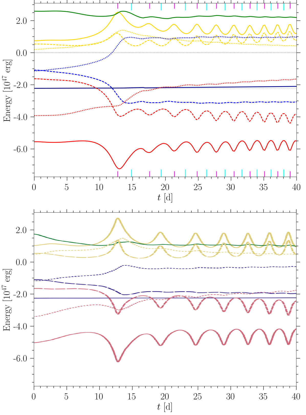
Figure 7: Comparison between energy terms (integrated over the simulation domain) in our simulation (top) and in the simulation of Ohlmann et al. (2016) (bottom, adapted from the latter work). Legend labels are the same as those of Ohlmann et al. (2016): ‘total’ (solid blue), ‘kinetic’ (solid yellow), ‘potential’ (solid red), ‘internal’ (solid green), ‘total envelope’ (dotted blue), ‘kinetic envelope’ (dotted yellow), ‘potential envelope’ (dotted red), ‘total cores’ (dashed blue), ‘kinetic cores’ (dashed yellow) and ‘potential cores’ (dashed red). In the upper panel the contribution from $E_{\mathrm{pot,gas-1}}$ is included in the envelope potential energy and total envelope energy but the contribution from $E_{\mathrm{pot,gas-2}}$ is not so included. On the other hand, the contribution from $E_{\mathrm{pot,gas-2}}$ is included in the cores potential energy and total cores energy, but these terms do not include the contribution from $E_{\mathrm{pot,gas-1}}$.

We used almost the same parameter values and initial conditions as Ohlmann et al. (2016) and thus it is useful to compare directly their results and ours. In the top panel of Fig. 7 we plot the energy terms as in Fig. 2 of Ohlmann et al. (2016), and in the bottom panel we show a version of their figure with the time axis truncated at $t=40\,{\rm d}$. The curves are as described in the legend but Ohlmann et al. (2016) used a different kind of code and it was not entirely clear to us precisely how the different energy components were divided among the various curves. We found that close agreement was obtained if the curves labeled as envelope potential energy and total envelope energy (dotted red and dotted blue, respectively) include the contribution from $E_{\mathrm{pot,gas-1}}$ but not from $E_{\mathrm{pot,gas-2}}$, and the curves labeled as cores potential energy and total cores energy (dashed red and dashed blue, respectively) include the contribution from $E_{\mathrm{pot,gas-2}}$ but not from $E_{\mathrm{pot,gas-1}}$,

The Ohlmann et al. (2016) setup allowed for a much lower pressure and lower density ambient medium. Thus, to make a direct comparison with our simulation, it was necessary to subtract from each energy term the fraction contributed by the ambient medium (or by the gravitational interaction between the ambient medium and the other components); these quantities involving the ambient gas were assumed to remain constant for the duration of the simulation. The ambient energy inflow from the boundaries is measured to be negligible. As expected from the analysis of Paper I, close agreement between results from the two simulations is apparent, in spite of the very different methodologies used. There is, however, a larger separation between the total particle energy and total gas energy curves (shown in dashed blue and dotted blue, respectively) after plunge-in in the top panel of Fig. 7 as compared with the bottom panel. The particle and gas potential energies also experience larger changes during plunge-in (dashed and dotted red, respectively).

Assuming that our partitioning of the energy components mimics reasonably well that of Ohlmann et al. (2016), these differences could be caused by differences in initial conditions. Firstly, in our simulation the RG is not rotating with respect to the inertial frame of reference of the simulation, while in that of Ohlmann et al. (2016) the RG is initialized with a solid body rotation of $95\%$ of the orbital angular speed. (The reality would lie somewhere in between and can be estimated as $\sim 30\%$ of the orbital angular speed from the results of MacLeod et al. 2018b). In spite of this difference, however, the inter-particle separation $a$ reaches a smaller value ($<10\,\mathrm{R_{\odot}}$) at the first periastron passage in the simulation of Ohlmann et al. (2016) than in that of Paper I ($14\,\mathrm{R_{\odot}}$), even though the time of this first periastron passage (i.e. the end of plunge-in, as we have defined it) occurs at about $t=13\,{\rm d}$ in both simulations.

Secondly, Ohlmann et al. (2016) performed a relaxation run to set up their initial condition, while we did not, which would have led to differences in the initial stellar profiles (apart from the slight differences that would have already existed due to the slightly different mesa models employed). We note that some quantities, like internal energy (solid green) and total potential energy (solid red) remain approximately constant for the first $\sim 5\,{\rm d}$ in our simulation, while showing more variation in that of Ohlmann et al. (2016). This suggests that the RG is more stable in our simulation. Possible reasons are that we iterated over the RG core mass to obtain a smoother initial RG profile, we resolved the entire RG at the highest refinement level, and we used a denser and higher pressure ambient medium to stabilize the outer layers of the RG. The latter is a compromise since a larger ambient density and pressure complicates the analysis. Clearly, obtaining an initial condition that is both highly stable and physically realistic in CE simulations is computationally challenging. In any case, we are encouraged by the close agreement between the two simulations, and take this as confirmation that our results are physical, as opposed to being dominated by numerical artefacts.

Appendix B Comparison of 1D and 3D stellar profiles

In Fig. 8 we compare the MESA solution with the profile obtained from a radial cut of our initial RGB star at $t=0$, taken directly from the AstroBear mesh. From top to bottom, panels show the gas density, internal energy density and potential energy density (the latter is equal to $\mathcal{E}_{\mathrm{pot,gas-gas}}+\mathcal{E}_{\mathrm{pot,gas-1}}$, and thus excludes the contribution from the primary-secondary gravitational interaction as well as that from ambient-ambient self-gravity). For the internal energy, we have also plotted the profile that would obtain if the MESA equation of state (EoS) had been that of an ideal gas with $\gamma=5/3$ (the case $\mathcal{E}_{\mathrm{int,gas}}=\tfrac{3}{2}P_{\mathrm{gas}}$). The agreement between our initial condition and the MESA model is very good for $r>1\,\mathrm{R_{\odot}}$. Our density and pressure were designed to match the MESA profile for $r>r_{\mathrm{soft}}=2.4\,\mathrm{R_{\odot}}$ (see also Ohlmann et al., 2017). Thus, internal energy density closely matches the MESA profile if the EoS is replaced by an ideal gas EoS. Near the stellar surface, the AstroBear internal energy density profile transitions smoothly to the ambient value. The profile of $\mathcal{E}_{\mathrm{int,gas}}$, made by assuming an ideal gas EoS, is slightly lower than the actual MESA profile, especially at larger radius. The small differences between the internal energy density profiles for the actual MESA model and that assuming an ideal gas EoS can be attributed to convective energy.

The potential energy profile of our initial condition also much agrees with the MESA profile, being slightly larger in magnitude for $1\lesssim r/\!\,\mathrm{R_{\odot}}\lesssim 19$, and slightly smaller at larger radii.

To assess how unbound our envelope is compared with that in the MESA model, we compute the total internal energy $E_{\mathrm{int,gas}}$ as well as the total energy $E_{\mathrm{int,gas}}+E_{\mathrm{pot,gas-gas}}+E_{\mathrm{pot,gas-1}}$ by integrating the profiles from $r_{\mathrm{soft}}=1\,\mathrm{R_{\odot}}$ to the stellar surface $R_{\mathrm{1}}=48.1\,\mathrm{R_{\odot}}$. For the MESA model we obtain $E_{\mathrm{int,gas}}=2.32\times 10^{47}\,{\rm erg}$ and $E_{\mathrm{int,gas}}+E_{\mathrm{pot,gas-gas}}+E_{\mathrm{pot,gas-1}}=-1.29\times 10^{47}\,{\rm erg}$. For the MESA model with ideal EoS we obtain $E_{\mathrm{int,gas}}=1.78\times 10^{47}\,{\rm erg}$ and $E_{\mathrm{int,gas}}+E_{\mathrm{pot,gas-gas}}+E_{\mathrm{pot,gas-1}}=-1.83\times 10^{47}\,{\rm erg}$. Finally, for our initial condition we obtain $E_{\mathrm{int,gas}}=1.76\times 10^{47}\,{\rm erg}$ and $E_{\mathrm{int,gas}}+E_{\mathrm{pot,gas-gas}}+E_{\mathrm{pot,gas-1}}=-1.92\times 10^{47}\,{\rm erg}$. Thus, the net energy terms in our initial condition closely match those of the MESA model if the EoS is replaced by the ideal gas EoS, as in our setup.

If, for example, we adopt $r=1\,\mathrm{R_{\odot}}$ as the location of the core-envelope boundary, the envelope in our initial condition is more strongly bound than that of the actual MESA model by about $0.6\times 10^{47}\,{\rm erg}$. This difference is insensitive to the location of the core-envelope boundary for $r>0.1\,\mathrm{R_{\odot}}$. This suggests that the unbound mass obtained in our simulation may be somewhat smaller than that which would be obtained with a more realistic initial condition.

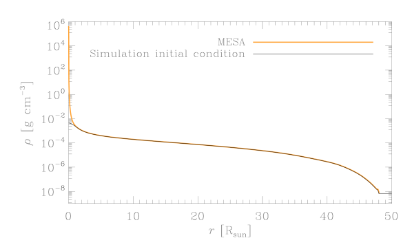
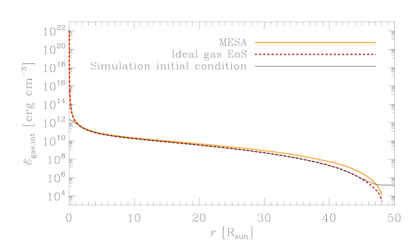
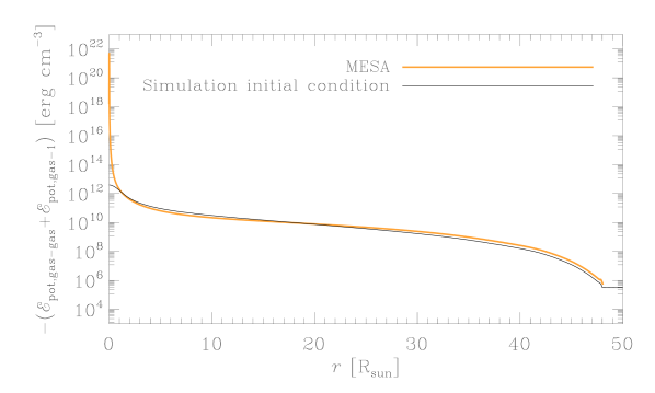
Figure 8: Top panel: Radial profiles of gas density for the RGB star modeled using MESA (thick orange) and the profile of our 3D RGB star in the simulation at $t=0$ (thin black). Middle panel: Comparison of the internal energy density profiles in the MESA model, simulation initial condition, and MESA model with the equation of state replaced with an ideal gas equation of state, as in the simulation (dashed red). Bottom panel: Comparison of (negative of) potential energy density profiles in the MESA model and simulation initial condition.

Appendix C Convergence tests

To test the dependence of the results on the parameters used in our numerical setup we performed five additional runs. The parameter values of the runs, including the fiducial run (Model A), are listed in Tab. 5.

Models B and C were designed to test the dependence of the results on the radius $r_{\mathrm{ref}}$ of the spherical region around the particles that was refined at the highest resolution $\delta$. Both runs employ smaller values of $r_{\mathrm{ref}}$ than that of the fiducial run at any given time. The orbit of Model B is remarkably similar to that of Model A until $t=16.7\,{\rm d}$, when $r_{\mathrm{ref}}$ becomes particularly small compared to Model A (and perhaps slightly before that time), but the period increases only slightly as a result. In Model C, the simulation is restarted from a frame of Model A at $t=24.1\,{\rm d}$ and runs for $3.0\,{\rm d}$ with a smaller value of $r_{\mathrm{ref}}$. The orbit is almost identical to that of Model A. These results suggest that the refinement region in the fiducial run is somewhat larger than what is actually required, and we could afford to be less conservative in the future.

Models D-F were designed to test the effects of changing the softening length $r_{\mathrm{soft}}$ (always equal for both particles) and/or the smallest resolution element $\delta$. The results for the orbital separation $a$ as a function of time are shown in Fig. 10. In Model A, both the softening length $r_{\mathrm{soft}}$ and the smallest resolution element $\delta$ are halved at $t=16.7\,{\rm d}$. In Model D (dashed-dotted), the softening length is halved at $t=16.7\,{\rm d}$ as in Model A, but the size of the smallest resolution element is kept constant. Before $t\approx 22\,{\rm d}$, the orbit matches closely to that of Model A. Thereafter, the amplitude of the separation curve reduces compared to that of Model A, and the mean separation increases at late times, while the period also slightly increases. By contrast, in Model E (dashed), where $\delta$ is halved as in Model A but $r_{\mathrm{soft}}$ is not, the amplitude is slightly larger than in Model A while the period and mean separation deviate only modestly from those of Model A (though Model E was terminated earlier than the other runs). Finally, in Model F (dotted) neither $r_{\mathrm{soft}}$ nor $\delta$ is halved, unlike in Model A, where both are halved. This run leads to an orbit that deviates from Model A more than Model E but less than Model D. Model F has a smaller period than Model A but a comparable amplitude, while the mean separation at late times is slightly smaller than for Model A.

Combining the results from Models A, D, E and F, we infer that: (i) at later times (and smaller separations), the mean separation and separation amplitude are sensitive to the number of resolution elements per softening length. A smaller value of $r_{\mathrm{soft}}/\delta$ (e.g. $\sim 9$ in Model D compared to $\sim 17$ in Model A) can lead to a larger mean separation, smaller separation amplitude, and larger period; (ii) For a given value of $r_{\mathrm{soft}}/\delta$, larger values of $r_{\mathrm{soft}}$ and $\delta$ tend to reduce the period and reduce the mean separation slightly, while hardly affecting the amplitude. We caution, however, that effects of changing the softening length cannot be attributed to numerics only because decreasing the softening length increases the gravitational force near the particles, which can result in a higher concentration of mass around the particles (Paper I).

Table 5: Parameters of the various models. Model A is the main model studied in this work while Models B through F are for testing. Parameters are the start or restart time of the simulation $t_{\mathrm{i}}$, the end time of the simulation $t_{\mathrm{f}}$, the spline softening length $r_{\mathrm{soft}}$, the size of the resolution element at the highest refinement level $\delta$, and the radius of the spherical volume within which cells are refined at the highest level $r_{\mathrm{ref}}$. For $t\leq 16.7\,{\rm d}$, this sphere is centred on particle 1 while for $t>16.7\,{\rm d}$ it is centred on particle 2 (in all models). For Models A and B, values of $r_{\mathrm{soft}}$ and $\delta$ are given for $t>16.7\,{\rm d}$. For $t\leq 16.7\,{\rm d}$ $r_{\mathrm{soft}}=2.4\,\mathrm{R_{\odot}}$ and $\delta=0.14\,\mathrm{R_{\odot}}$ for those models.

Model	$t_{\mathrm{i}}$	$t_{\mathrm{f}}$	$r_{\mathrm{soft}}$	$\delta$	$r_{\mathrm{soft}}/\delta$	$r_{\mathrm{ref}}$
	$[\!\,{\rm d}]$	$[\!\,{\rm d}]$	$[\!\,\mathrm{R_{\odot}}]$	$[\!\,\mathrm{R_{\odot}}]$
A	$0$	$40.0$	$1.2$	$0.07$	$17$	Fiducial
B	$0$	$22.0$	$1.2$	$0.07$	$17$	Small
C	$24.1$	$27.1$	$1.2$	$0.07$	$17$	Small
D	$16.7$	$35.6$	$1.2$	$0.14$	$9$	Fiducial
E	$16.7$	$32.4$	$2.4$	$0.07$	$34$	Fiducial
F	$16.7$	$37.3$	$2.4$	$0.14$	$17$	Fiducial

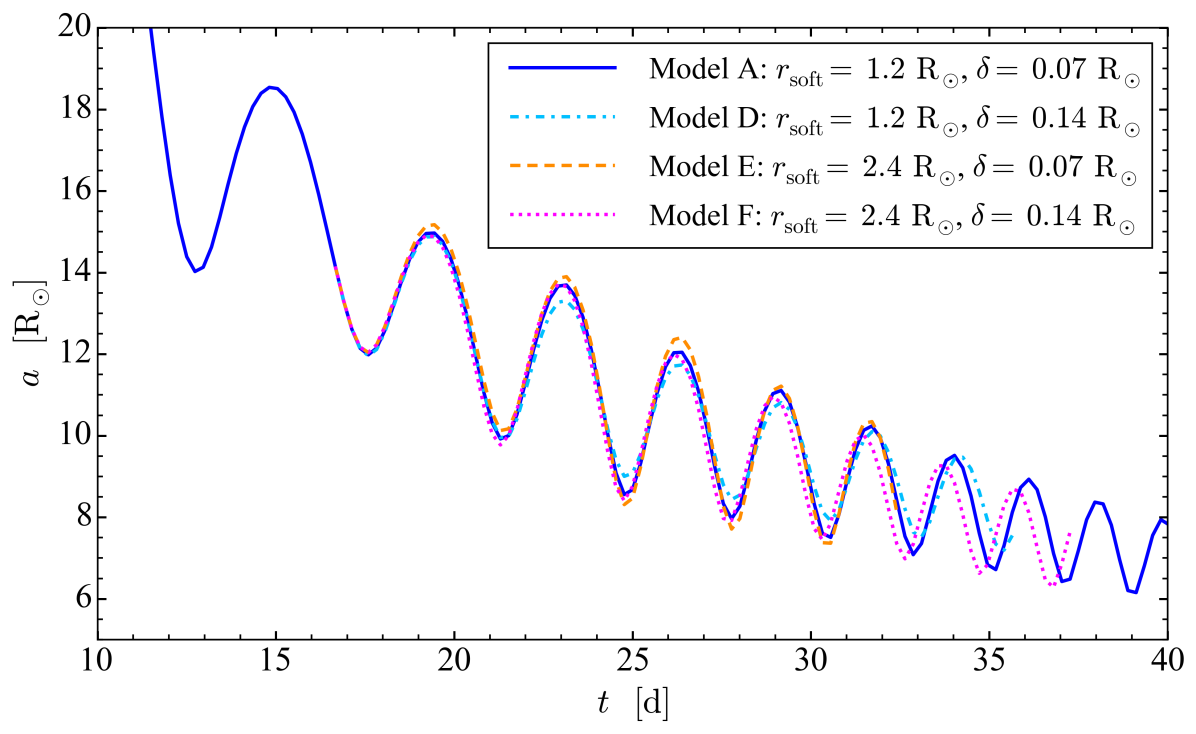
Figure 10: Orbital separation $a$ between particles 1 and 2 for the fiducial run, Model A (solid blue), Model D, restarted from Model A from $t=16.7\,{\rm d}$ but without halving $\delta$ (dashed-dotted light blue), Model E, restarted from Model A from $t=16.7\,{\rm d}$ but without halving $r_{\mathrm{soft}}$ (dashed orange), and Model F, restarted from Model A from $t=16.7\,{\rm d}$ but without halving either $\delta$ or $r_{\mathrm{soft}}$ (dotted magenta).

References

- Briggs et al. (2018) Briggs G. P., Ferrario L., Tout C. A., Wickramasinghe D. T., 2018, MNRAS, 481, 3604
- Carroll-Nellenback et al. (2013) Carroll-Nellenback J. J., Shroyer B., Frank A., Ding C., 2013, Journal of Computational Physics, 236, 461
- Chamandy et al. (2018) Chamandy L., et al., 2018, MNRAS, 480, 1898
- Clayton et al. (2017) Clayton M., Podsiadlowski P., Ivanova N., Justham S., 2017, MNRAS, 470, 1788
- Clyne et al. (2014) Clyne N., Redman M. P., Lloyd M., Matsuura M., Singh N., Meaburn J., 2014, A&A, 569, A50
- Cojocaru et al. (2017) Cojocaru R., Rebassa-Mansergas A., Torres S., García-Berro E., 2017, MNRAS, 470, 1442
- Cunningham et al. (2009) Cunningham A. J., Frank A., Varnière P., Mitran S., Jones T. W., 2009, ApJS, 182, 519
- Davis et al. (2010) Davis P. J., Kolb U., Willems B., 2010, MNRAS, 403, 179
- Dewi & Tauris (2000) Dewi J. D. M., Tauris T. M., 2000, A&A, 360, 1043
- Eggleton (1983) Eggleton P. P., 1983, ApJ, 268, 368
- Hillwig et al. (2016) Hillwig T. C., Jones D., De Marco O., Bond H. E., Margheim S., Frew D., 2016, ApJ, 832, 125
- Iaconi et al. (2017) Iaconi R., Reichardt T., Staff J., De Marco O., Passy J.-C., Price D., Wurster J., Herwig F., 2017, MNRAS, 464, 4028
- Iaconi et al. (2018) Iaconi R., De Marco O., Passy J.-C., Staff J., 2018, MNRAS, 477, 2349
- Ivanova & Nandez (2016) Ivanova N., Nandez J. L. A., 2016, MNRAS, 462, 362
- Ivanova et al. (2013) Ivanova N., et al., 2013, ARA&A, 21, 59
- Jones et al. (2010) Jones D., et al., 2010, MNRAS, 408, 2312
- Jones et al. (2015) Jones D., Boffin H. M. J., Rodríguez-Gil P., Wesson R., Corradi R. L. M., Miszalski B., Mohamed S., 2015, A&A, 580, A19
- Livio & Soker (1988) Livio M., Soker N., 1988, ApJ, 329, 764
- MacLeod et al. (2018a) MacLeod M., Ostriker E. C., Stone J. M., 2018a, preprint, (arXiv:1808.05950)
- MacLeod et al. (2018b) MacLeod M., Ostriker E. C., Stone J. M., 2018b, ApJ, 863, 5
- McLean et al. (2001) McLean A. A., Guerrero M. A., Gruendl R. A., Chu Y. H., 2001, in American Astronomical Society Meeting Abstracts. p. 1509
- Metzger & Pejcha (2017) Metzger B. D., Pejcha O., 2017, MNRAS, 471, 3200
- Miszalski et al. (2018) Miszalski B., Manick R., Mikołajewska J., Van Winckel H., Iłkiewicz K., 2018, PASA, 35, e027
- Nandez & Ivanova (2016) Nandez J. L. A., Ivanova N., 2016, MNRAS, 460, 3992
- Nandez et al. (2014) Nandez J. L. A., Ivanova N., Lombardi Jr. J. C., 2014, ApJ, 786, 39
- Ohlmann et al. (2016) Ohlmann S. T., Röpke F. K., Pakmor R., Springel V., 2016, ApJ, 816, L9
- Ohlmann et al. (2017) Ohlmann S. T., Röpke F. K., Pakmor R., Springel V., 2017, A&A, 599, A5
- Passy et al. (2012) Passy J.-C., Mac Low M.-M., De Marco O., 2012, ApJ, 759, L30
- Paxton et al. (2011) Paxton B., Bildsten L., Dotter A., Herwig F., Lesaffre P., Timmes F., 2011, ApJS, 192, 3
- Paxton et al. (2013) Paxton B., et al., 2013, ApJS, 208, 4
- Paxton et al. (2015) Paxton B., et al., 2015, ApJS, 220, 15
- Rasio & Livio (1996) Rasio F. A., Livio M., 1996, ApJ, 471, 366
- Reichardt et al. (2018) Reichardt T. A., De Marco O., Iaconi R., Tout C. A., Price D. J., 2018, preprint, (arXiv:1809.02297)
- Ricker & Taam (2012) Ricker P. M., Taam R. E., 2012, ApJ, 746, 74
- Sahai et al. (1999) Sahai R., et al., 1999, AJ, 118, 468
- Sandquist et al. (1998) Sandquist E. L., Taam R. E., Chen X., Bodenheimer P., Burkert A., 1998, ApJ, 500, 909
- Sandquist et al. (2000) Sandquist E. L., Taam R. E., Burkert A., 2000, ApJ, 533, 984
- Soker (1999) Soker N., 1999, MNRAS, 303, 611
- Tutukov & Yungelson (1979) Tutukov A., Yungelson L., 1979, in Conti P. S., De Loore C. W. H., eds, IAU Symposium Vol. 83, Mass Loss and Evolution of O-Type Stars. pp 401–406
- Zorotovic et al. (2010) Zorotovic M., Schreiber M. R., Gänsicke B. T., Nebot Gómez-Morán A., 2010, A&A, 520, A86
- de Kool (1990) de Kool M., 1990, ApJ, 358, 189
- van den Heuvel (1976) van den Heuvel E. P. J., 1976, in Eggleton P., Mitton S., Whelan J., eds, IAU Symposium Vol. 73, Structure and Evolution of Close Binary Systems. p. 35