Differential Temporal Difference Learning

Abstract

Value functions derived from Markov decision processes arise as a central component of algorithms as well as performance metrics in many statistics and engineering applications of machine learning. Computation of the solution to the associated Bellman equations is challenging in most practical cases of interest. A popular class of approximation techniques, known as Temporal Difference (TD) learning algorithms, are an important sub-class of general reinforcement learning methods. The algorithms introduced in this work are intended to resolve two well-known issues with TD-learning algorithms: Their slow convergence due to very high variance, and the fact that, for the problem of computing the relative value function, consistent algorithms exist only in special cases. First we show that the gradients of these value functions admit a representation that lends itself to algorithm design. Based on this result, a new class of differential TD-learning algorithms is introduced. For Markovian models on Euclidean space with smooth dynamics, the algorithms are shown to be consistent under general conditions. Numerical results show dramatic variance reduction in comparison to standard methods.

Keywords: Reinforcement learning, approximate dynamic programming, temporal difference learning, Poisson equation, stochastic optimal control

1 Introduction

A central task in the application of many machine learning methods and control techniques is the (exact or approximate) computation of value functions arising from Markov decision processes. The class of Temporal Difference (TD) learning algorithms considered in this work is an important sub-class of the general family of reinforcement learning methods that performs this task. Our main contributions here are the introduction of a related family of TD-learning algorithms that enjoy better convergence properties than existing methods, and the rigorous theoretical analysis of these algorithms.

The value functions considered in this work are based on a discrete-time Markov chain ${\mbox{\boldmath$X$}}=\{X(t):t=0,1,2,\ldots\}$ taking values in ${\mathbb{R}}^{\ell}$, and on an associated cost function $c:{\mathbb{R}}^{\ell}\to{\mathbb{R}}$. Our central modelling assumption throughout is that $X$ evolves according to the nonlinear state space model,

$$X(t+1)=a(X(t),N(t+1)),\quad t\geq 0,$$ (1)

where ${\mbox{\boldmath$N$}}\!=\!\{N(t)\!:\!t\!=\!0,1,2,\ldots\}$ is an $m$-dimensional disturbance sequence of independent and identically distributed (i.i.d.) random variables, and $a:{\mathbb{R}}^{\ell+m}\to{\mathbb{R}}^{\ell}$ is a continuous mapping. Under these assumptions, for all $t\geq 0$, $X(t+1)$ is a continuous function of the initial condition $X(0)=x$; this observation is our starting point for the construction of effective algorithms for value function approximation.

We begin with some familiar background.

1.1 Value functions

Given a discount factor $\beta\in(0,1)$, the discounted-cost value function is defined as

$$h_{\beta}(x)\mathbin{:=}\sum_{t=0}^{\infty}\beta^{t}{\sf E}[c(X(t))\mid X(0)=x]\,,\qquad x\in{\mathbb{R}}^{\ell}.$$ (2)

It is known that $h_{\beta}$ solves the Bellman equation [2, 3]:

$$c(x)+\beta{\sf E}[h_{\beta}(X(t+1))|X(t)=x]-h_{\beta}(x)=0\,.$$ (3)

The average cost is defined as the ergodic limit,

$$\eta\mathbin{:=}\lim_{n\rightarrow\infty}\frac{1}{n}\sum_{t=0}^{n-1}{\sf E}[c(X(t))\mid X(0)=x]\,,$$ (4)

where the limit exists and is independent of $x$ under the conditions discussed in Section 2. The following relative value function is central to analysis of average cost control problems:

$$h(x)\mathbin{:=}\sum_{t=0}^{\infty}{\sf E}[c(X(t))-\eta\mid X(0)=x]\,,\qquad x\in{\mathbb{R}}^{\ell}.$$ (5)

Provided the sum (5) exists for each $x$, the relative value function solves the Poisson equation [6, 3]:

$${\sf E}[h(X(t+1))\mid X(t)=x]-h(x)=-[c(x)-\eta]\,.$$ (6)

These equations and their solutions are of interest in learning theory, control engineering, and many other fields, including:

Optimal control and Markov decision processes: Policy iteration and actor-critic algorithms are designed to approximate an optimal policy using two-step procedures: First, given a policy, the associated value function is computed (or approximated), and then the policy is updated based on this value function [7, 8]. These approaches can be used for both discounted- and average-cost optimal control problems.

Algorithm design for variance reduction: Under general conditions, the asymptotic variance (i.e., the variance appearing in the central limit theorem for the averages in (4)) is naturally expressed in terms of the relative value function $h$ [9, 10]. The method of control variates is intended to reduce the asymptotic variance of various Monte Carlo methods; a version of this technique involves the construction of an approximation to $h$ [11, 12, 13, 14, 15].

Nonlinear filtering: A recent approach to approximate nonlinear filtering requires the gradient of the solution to Poisson’s equation to obtain the “innovation gain” [16, 17]. Approximations of the solution can lead to efficient implementations of this method [18, 19, 20].

1.2 TD-learning and value function approximation

In most cases of practical interest, closed-form expressions for the value functions $h_{\beta}$ and $h$ in (2) or (6) cannot be derived. One approach to obtaining approximations is the Temporal Difference (TD) learning algorithm [21, 2].

In the case of the discounted-cost value function, the goal of TD-learning is to approximate $h_{\beta}$ as a member of a parametrized family of functions $\{h_{\beta}^{\theta}:\theta\in{\mathbb{R}}^{d}\}$. Throughout, we restrict attention to linear parametrizations of the form,

$$h_{\beta}^{\theta}=\sum_{j=1}^{d}\theta_{j}\psi_{j},$$ (7)

where we write $\theta=(\theta_{1},\theta_{2},\ldots,\theta_{d})^{\hbox{\tiny\it T}}$, $\psi=(\psi_{1},\psi_{2},\ldots,\psi_{d})^{\hbox{\tiny\it T}}$, and we assume that the given collection of ‘basis’ functions $\psi\colon{\mathbb{R}}^{\ell}\to{\mathbb{R}}^{d}$ is continuously differentiable.

For any function $f:{\mathbb{R}}^{\ell}\to{\mathbb{R}}$, and a given probability measure $\mu:{\mathbb{R}}^{\ell}\to[0,1]$, we define the $\mu$-norm:

$$\|f\|_{\mu} \mathbin{:=}\Big{(}{\sf E}[f^{2}(X)]\Big{)}^{{\mathchoice{\genfrac{}{}{}{1}{1}{2}}{\genfrac{}{}{}{1}{1}{2}}{\genfrac{}{}{}{3}{1}{2}}{\genfrac{}{}{}{3}{1}{2}}}}\,,\quad X\sim\mu$$

$$=\Big{(}\int f^{2}(x)\mu(dx)\Big{)}^{{\mathchoice{\genfrac{}{}{}{1}{1}{2}}{\genfrac{}{}{}{1}{1}{2}}{\genfrac{}{}{}{3}{1}{2}}{\genfrac{}{}{}{3}{1}{2}}}}$$

In one variant of the TD technique (the LSTD(1) algorithm, described in Section 4), the optimal parameter vector $\theta^{*}$ is chosen as the solution to a minimum-norm problem,

$$\theta^{*} =\mathop{\rm arg\,min}_{\theta}\|h_{\beta}^{\theta}-h_{\beta}\|^{2}_{\pi}$$ (8)

where the expectation is with respect to $X\sim\pi$, and $\pi$ denotes the steady-state distribution of the Markov chain $X$; more details are provided in Sections 2.1 and 4.

A TD-learning algorithm is said to be consistent, if the parameter estimates obtained using the algorithm converge to $\theta^{*}$.

Theory for TD-learning in the discounted-cost setting is largely complete, in the sense that criteria for convergence are well-understood, and the asymptotic variance of the algorithm is computable based on standard theory from stochastic approximation [22, 23, 25] ; see [4, 24, 5] for the relationship between asymptotic variance and convergence rate of TD-learning algorithms. Theory and algorithms for the average-cost setting involving the relative value function $h$ is more fragmented. The optimal parameter $\theta^{*}$ in the analog of (8) with $h_{\beta}$ replaced by the relative value function $h$ can be computed using TD-learning techniques only for Markovian models that regenerate: there exists a state $x^{\bullet}\in{\mathbb{R}}^{\ell}$ that is visited infinitely often (see the regenerative TD($1$) algorithm in [43, pg. 1012], and also [3, 26]).

Regeneration is often not a restrictive assumption. However, the asymptotic variance of these algorithms grows with the variance of inter-regeneration times (time between consecutive visits to the regenerative state $x^{\bullet}$). The variance can be massive even in simple examples such as the M/M/1 queue; see the final chapter of [3]. High variance is also predominantly observed in the discounted-cost case when the discounting factor is close to $1$; see the relevant remarks in Section 1.4.

The differential TD-learning algorithms developed in this paper are designed in part to resolve these issues. The main idea is to estimate the gradient of the value function. Under the conditions imposed, the asymptotic variance of the resulting algorithms remains uniformly bounded over $0<\beta<1$. And the same techniques can be applied to obtain finite-variance algorithms for approximating the relative value function $h$ for models without regeneration.

We note that the needs of the analysis of the algorithms presented here have, in part, motivated the development of rich new convergence theory for general classes of Markov processes [28]. Indeed, the results in Sections 2 and 3 draw heavily on the convergence results established in [28].

1.3 Differential TD-learning

Consider the discounted-cost setting; suppose that the value function $h_{\beta}$ and all its potential approximations $\{h_{\beta}^{\theta}:\theta\in{\mathbb{R}}^{d}\}$ are continuously differentiable as functions of the state $x$, i.e., $h_{\beta},\,h_{\beta}^{\theta}\,\in C^{1}$, for each $\theta\in{\mathbb{R}}^{d}$. In terms of the linear parametrization (7), we obtain approximations of the form:

$$\nabla h_{\beta}^{\theta}=\sum_{j=1}^{d}\theta_{j}\nabla\psi_{j}\,,$$ (9)

where the gradient is with respect to the state $x$.

The differential LSTD-learning algorithm introduced in Section 3 is designed to compute the solution to

$$\theta^{*}=\mathop{\rm arg\,min}_{\theta}{\sf E}[\|\nabla h_{\beta}^{\theta}(X)-\nabla h_{\beta}(X)\|_{2}^{2}]\,,\quad X\sim\pi\,,$$ (10)

where $\|\cdot\|_{2}$ is the usual Euclidean norm, and once again, $\pi$ denotes the steady-state distribution of the Markov chain $X$.

The value function approximation $h_{\beta}^{\theta^{*}}$ is obtained via the addition of a constant:

$$h_{\beta}^{\theta^{*}}=\sum_{j=1}^{d}\theta_{j}^{*}\psi_{j}+\kappa(\theta^{*}).$$ (11)

The mean-square optimal choice is obtained on requiring

$${\sf E}[h_{\beta}^{\theta^{*}}(X)-h_{\beta}(X)]=0\,,\quad X\sim\pi\,.$$ (12)

See the discussion that follows Algorithm 2 for details.

A similar program can be carried out for the relative value function $h$, which, viewed as a solution to Poisson’s equation (6), is unique only up to an additive constant. Therefore, we can set $\kappa(\theta^{*})=0$ in the average-cost setting.

1.4 Summary of contributions

The main contributions of this work are:

$(i)$ The introduction of the new differential Least Squares TD-learning ($\nabla$-LSTD, or ‘grad-LSTD’) algorithm, which is applicable in both the discounted- and average-cost settings.

$(ii)$ The development of appropriate conditions under which we can show that, for linear parametrizations, $\nabla$-LSTD converges and solves the quadratic program (10).

$(iii)$ The introduction of the family of $\nabla$-LSTD($\lambda$)-learning algorithms. It is shown that $\nabla$-LSTD($1$) also solves the quadratic program (10).

$(iv)$ These new algorithms are applicable for models that do not have regeneration. Their asymptotic variance is uniformly bounded over all $0<\beta<1$, under general conditions.

Perhaps the most important limitation of the $\nabla$-LSTD algorithms is the requirement of partial knowledge of the Markov chain transition dynamics. Section 6 contains discussion on how to address this challenge. Fortunately, in many applications, very little knowledge is required (such as in the queuing example discussed in Section 5.2).

Finally, a few more remarks about the error rates of these algorithms are in order. From the definition of the value function (2), it can be expected that $h_{\beta}(x)\to\infty$ as $\beta\to 1$ for each $x\in{\mathbb{R}}^{\ell}$. This is why approximation methods in reinforcement learning typically take for granted that error will grow at this rate. Moreover, it is observed that variance in reinforcement learning can grow dramatically with the discount factor. In particular, it is shown in [23, 24] that asymptotic variance in the standard Q-learning algorithm of Watkins is infinite when the discount factor satisfies $\beta>1/2$.

The family of TD($\lambda$) algorithms was introduced in [21] to reduce the variance of earlier methods, but it brings its own potential challenges. Consider [29, Theorem 1], which compares the estimate $h^{\theta^{\lambda}}_{\beta}$ obtained using TD($\lambda$), with the $L_{2}$-optimal approximation $h^{\theta^{*}}_{\beta}$ obtained using TD($1$):

$$\|h^{\theta^{\lambda}}_{\beta}-h_{\beta}\|_{\pi}\leq\frac{1-\lambda\beta}{1-\beta}\|h^{\theta^{*}}_{\beta}-h_{\beta}\|_{\pi}.$$ (13)

This bound suggests that the bias can grow as $(1-\beta)^{-1}$.

The difficulties are more acute when we come to the average-cost problem. Consider the minimum-norm problem (8) with the relative value function $h$ in place of $h_{\beta}$:

$$\theta^{*}=\mathop{\rm arg\,min}_{\theta}\|h^{\theta}-h\|^{2}_{\pi}.$$ (14)

Here, for the TD($\lambda$) algorithm with $\lambda<1$, Theorem 3 of [6] implies a bound in terms of the “convergence rate” $\rho$ for the Markov chain,

$$\|h^{\theta^{\lambda}}_{\beta}-h\|_{\pi}\leq c(\lambda,\rho)\|h^{\theta^{*}}-h\|_{\pi},$$ (15)

in which $c(\lambda,\rho)>1$ and $c(\lambda,\rho)\to 1$ as $\lambda\to 1$.

Convergence of TD($1$) does not hold for the average cost problem. Specialized algorithms making use of regeneration were introduced in [43, pg. 1012], [3, 26].

For any differentiable function function $f:{\mathbb{R}}^{\ell}\to{\mathbb{R}}$, its gradient is denoted

$$\nabla f\mathbin{:=}\Big{[}\frac{\partial}{\partial x_{1}}f\,,\ldots\,,\frac{\partial}{\partial x_{\ell}}f\Big{]}^{\hbox{\tiny\it T}}$$ (16)

Under the assumptions imposed in this paper, we show that the gradients of the value functions are well behaved: $\{\nabla h_{\beta}:0<\beta\leq 1\}$ is a bounded collection of functions, and $\nabla h_{\beta}\to\nabla h$ uniformly on compact sets. As a consequence, both the bias and variance of the new $\nabla$-LSTD($\lambda$) algorithms are bounded over all $0<\beta\leq 1$.

The remainder of the paper is organized as follows: Basic definitions and value function representations are presented in Section 2. The $\nabla$-LSTD-learning algorithm is introduced in Section 3, and the family of $\nabla$-LSTD($\lambda$) algorithms are introduced in Section 4. Results from numerical experiments are shown in Section 5, and conclusions are contained in Section 6.

2 Representations and Approximations

We begin with modelling assumptions on the Markov process $X$, and representations for the value functions $h_{\beta},h$ and their gradients.

2.1 Markovian model and value function gradients

The evolution equation (1) defines a Markov chain $X$ with transition semigroup $\{P^{t}\}$, where $P^{t}(x,A)$ is defined, for all $t\geq 0$, any state $x\in{\mathbb{R}}^{\ell}$, and every measurable $A\subset{\mathbb{R}}^{\ell}$, via,

$$P^{t}(x,A):={\sf P}_{x}\{X(t)\in A\}:=\Pr\{X(t)\in A\,|\,X(0)=x\}.$$

For $t=1$ we write $P=P^{1}$, so that:

$$P(x,A)=\Pr\{a(x,N(1))\in A\}\,,$$

where we recall that $a:{\mathbb{R}}^{\ell+m}\to{\mathbb{R}}^{\ell}$ defines the dynamics of the Markov chain in (1).

The first set of assumptions ensures that the value functions $h_{\beta}$ and $h$ are well-defined. Fix a continuous function $v\colon{\mathbb{R}}^{\ell}\to[1,\infty)$ that serves as a weighting function. For any measurable function $f\colon{\mathbb{R}}^{\ell}\to{\mathbb{R}}$, the $v$-norm is defined as follows:

$$\|f\|_{v}\mathbin{:=}\sup_{x}\frac{|f(x)|}{v(x)}\,,$$

and the associated Banach space is denoted

$$L_{\infty}^{v}\mathbin{:=}\{f:{\mathbb{R}}^{\ell}\to{\mathbb{R}}:\|f\|_{v}<\infty\}.$$

Also, for any measurable function $f$ and measure $\mu$, we write $\mu(f)$ for the integral, $\mu(f):=\int fd\mu.$

Assumption A1:

• The Markov chain $X$ is $v$-uniformly ergodic: It has a unique invariant probability measure $\pi$, and there exists a continuous function $v:{\mathbb{R}}^{\ell}\to{\mathbb{R}}$ and constants $b_{0}<\infty$ and $0<\rho_{0}<1$, such that, for each function $f\in L_{\infty}^{v}$,

  $$\Big{|}{\sf E}\big{[}f(X(t))\mid X(0)=x\big{]}-\pi(f)\Big{|}\leq b_{0}\rho_{0}^{t}\|f\|_{v}v(x),$$

  for all $x\in{\mathbb{R}}^{\ell},\,t\geq 0$

Assumption A1 is not a strong assumption: it is essentially equivalent to geometric ergodicity in the usual sense (ignoring a set of measure zero): combine Theorems 15.0.2 and 16.0.1 of [10]. There is also an exact equivalence between Assumption A1 and the existence of a “Lyapunov function” [10, Theorem 16.0.1]. See [10] and Section 5 of this paper for examples where the assumption holds.

The following consequences are immediate [10, 3]:

Proposition 2.1.

Under assumption A1, for any cost function $c$ such that $\|c\|_{v}<\infty$, the limit $\eta$ in (4) exists with $\eta:=\pi(c)<\infty$, and is independent of the initial state $x$. The value functions $h_{\beta}$ and $h$ exist as expressed in (2) and (5), and they satisfy equations (3) and (6), respectively.

Moreover, there exists a constant $b_{c}<\infty$ such that the following bounds hold:

$$|h(x)| \leq b_{c}v(x)$$

$$|h_{\beta}(x)| \leq b_{c}\big{(}v(x)+(1-\beta)^{-1}\big{)}$$

$$|h_{\beta}(x)-h_{\beta}(y)| \leq b_{c}\big{(}v(x)+v(y)\big{)}\,,\qquad\qquad x,y\in{\mathbb{R}}^{\ell}.$$

The following operator-theoretic notation will simplify exposition throughout. For any measurable function $f\colon{\mathbb{R}}^{\ell}\to{\mathbb{R}}$, the new function $P^{t}f:{\mathbb{R}}^{\ell}\to{\mathbb{R}}$ is defined as the conditional expectation:

$$P^{t}f\,(x)={\sf E}_{x}[f(X(t))]\mathbin{:=}{\sf E}[f(X(t))\mid X(0)=x].$$

For any $\beta\in(0,1)$, the resolvent kernel $R_{\beta}$ is the “$z$-transform” of the semigroup $\{P^{t}\}$,

$$R_{\beta}\mathbin{:=}\sum_{t=0}^{\infty}\beta^{t}P^{t}.$$ (17)

Under the assumptions of Prop. 2.1, the discounted-cost value function $h_{\beta}$ admits the representation,

$$h_{\beta}=R_{\beta}c\,,$$ (18)

and similarly, for the relative value function $h$ we have,

$$h=R[c-\eta],$$ (19)

where we write $R\equiv R_{\beta}$ when $\beta=1$ [10, 30, 3].

The representations (18) and (19) are valuable in deriving the LSTD-learning algorithms [2, 3, 31]. Analogous representations for the gradients are obtained in this paper:

$$\nabla h_{\beta}=\nabla[R_{\beta}c],\qquad\nabla h=\nabla[Rc]\,.$$

2.2 Representation for the gradient of a value function

In this section we describe the construction of operators $\Omega$ and $\Omega_{\beta}$, which satisfy the following:

$$\nabla h_{\beta}=\nabla[R_{\beta}c]=\Omega_{\beta}\nabla c\,,\quad\nabla h=\nabla[Rc]=\Omega\nabla c.$$ (20)

A more detailed account is given in Section 3.2, and a complete exposition of the underlying theory together with the formal justification of the existence and the relevant properties of $\Omega$ and $\Omega_{\beta}$ can be found in [28].

For the sake of simplicity, here we restrict our discussion to $h_{\beta}$ and its gradient. But it is not hard to see that the construction below easily generalizes to $\beta=1$; again, see Section 3.2 and [28] for the relevant details.

We require the following further assumptions:

Assumption A2:

• The process $N$ is independent of $X(0)$.

• The function $a$ is continuously differentiable in its first variable, with

  $$\sup_{x,n}\|\nabla_{x}a(x,n)\|<\infty,$$

  where $\|\,\cdot\,\|$ is any matrix norm, and the $\ell\times\ell$ matrix $\nabla_{x}a$ is defined as:

  $$[\nabla a_{x}(x,n)]_{i,j}\mathbin{:=}\frac{\partial}{\partial x_{i}}(a(x,n))_{j},\quad 1\leq i,j\leq\ell.$$

The first assumption, A2.1, is critical so that the initial state $X(0)=x$ can be regarded as a variable, with $X(t)$ a continuous function of $x$. This together with A2.2 allows us to define the sensitivity process $\{{\cal S}(t)\}$, where, for each $t\geq 0$:

$${\cal S}_{i,j}(t)\mathbin{:=}\frac{\partial X_{i}(t)}{\partial X_{j}(0)},\quad 1\leq i,j\leq\ell.$$ (21)

The evolution equations (1) imply that the sensitivity process evolves as a random linear system,

$${\cal S}(t+1) ={\cal A}(t+1){\cal S}(t),\quad t\geq 0,$$ (22)

with initial condition ${\cal S}(0)=I$, where the $\ell\times\ell$ matrix ${\cal A}(t)$ is defined as in assumption A2.2, by

$${\cal A}^{\hbox{\tiny\it T}}(t)\mathbin{:=}\nabla_{x}a\,(X(t-1),N(t))$$ (23)

For any $C^{1}$ function $f:{\mathbb{R}}^{\ell}\to{\mathbb{R}}$, denote

$$\nabla^{\cal S}\!f(X(t))\mathbin{:=}{\cal S}^{\hbox{\tiny\it T}}(t)\nabla f(X(t))\,.$$ (24)

It follows from the chain rule that this coincides with the gradient of $f(X(t))$ with respect to the initial condition $x$:

$$\big{[}\nabla^{\cal S}\!f(X(t))\big{]}_{i}=\frac{\partial f(X(t))}{\partial{X_{i}(0)}},\quad 1\leq i\leq\ell.$$ (25)

Equation (24) motivates the introduction of a semigroup $\{Q^{t}:t\geq 0\}$ of operators, whose domain includes functions $g:{\mathbb{R}}^{\ell}\to{\mathbb{R}}^{\ell}$ of the form $g=[g_{1},\ldots,g_{\ell}]^{{\hbox{\tiny\it T}}}$, with $g_{i}\in L_{\infty}^{v}$ for each $i$. For $t=0$, $Q^{0}$ is the identity operator, and for $t\geq 1$,

$$Q^{t}g(x)\mathbin{:=}{\sf E}_{x}\bigl{[}{\cal S}^{\hbox{\tiny\it T}}(t)g(X(t))\bigr{]}.$$ (26)

Provided we can exchange the gradient and the expectation, following (25), we have,

$$\frac{\partial}{\partial x_{i}}{\sf E}_{x}[f(X(t))]={\sf E}_{x}\bigl{[}[\nabla^{\cal S}\!f(X(t))]_{i}\bigr{]},\quad 1\leq i\leq\ell,$$

and consequently, the following elegant formula is obtained:

$$\nabla P^{t}f(x)={\sf E}_{x}[\nabla^{\cal S}\!f(X(t))]=Q^{t}\nabla f\,(x),\;\;\;x\in{\mathbb{R}}^{\ell}.$$ (27)

Justification requires minimal assumptions on the function $f$. The proof of Prop. 2.2 is based on Lemmas A.1 and A.2 contained in Appendix A.

Proposition 2.2.

Suppose that Assumptions A1 and A2 hold, and that $f^{2}$ and $\|\nabla f\|_{2}^{2}$ both lie in $L_{\infty}^{v}$. Then (27) holds, and $\nabla P^{t}f\,(x)$ is continuous as a function of $x\in{\mathbb{R}}^{\ell}$.

Proof.

The proof uses Lemma A.2 in the Appendix, and a variant of the truncation argument of [28]. Let $\{{\mathchoice{\mathord{\raisebox{1.5pt}{\scalebox{1.25}{$\chi$}}}}{\mathord{\raisebox{1.5pt}{\scalebox{1.25}{$\chi$}}}}{\mathord{\raisebox{1.0pt}{\scalebox{0.75}{$\chi$}}}}{\mathord{\raisebox{0.8pt}{\scalebox{0.6}{$\chi$}}}}}_{n}:n\geq 1\}$ be a sequence of functions satisfying, for each $n$:

• ${\mathchoice{\mathord{\raisebox{1.5pt}{\scalebox{1.25}{$\chi$}}}}{\mathord{\raisebox{1.5pt}{\scalebox{1.25}{$\chi$}}}}{\mathord{\raisebox{1.0pt}{\scalebox{0.75}{$\chi$}}}}{\mathord{\raisebox{0.8pt}{\scalebox{0.6}{$\chi$}}}}}_{n}$ is a continuous approximation to the indicator function on the set $R_{n}$, where

  $$R_{n}\mathbin{:=}\{x\in{\mathbb{R}}^{\ell}:|x_{i}|\leq n,\ \ 1\leq i\leq d\}\,,$$

  in the sense that $0\leq{\mathchoice{\mathord{\raisebox{1.5pt}{\scalebox{1.25}{$\chi$}}}}{\mathord{\raisebox{1.5pt}{\scalebox{1.25}{$\chi$}}}}{\mathord{\raisebox{1.0pt}{\scalebox{0.75}{$\chi$}}}}{\mathord{\raisebox{0.8pt}{\scalebox{0.6}{$\chi$}}}}}_{n}(x)\leq 1$ for all $x$, ${\mathchoice{\mathord{\raisebox{1.5pt}{\scalebox{1.25}{$\chi$}}}}{\mathord{\raisebox{1.5pt}{\scalebox{1.25}{$\chi$}}}}{\mathord{\raisebox{1.0pt}{\scalebox{0.75}{$\chi$}}}}{\mathord{\raisebox{0.8pt}{\scalebox{0.6}{$\chi$}}}}}_{n}(x)=1$ when $x\in R_{n}$, and ${\mathchoice{\mathord{\raisebox{1.5pt}{\scalebox{1.25}{$\chi$}}}}{\mathord{\raisebox{1.5pt}{\scalebox{1.25}{$\chi$}}}}{\mathord{\raisebox{1.0pt}{\scalebox{0.75}{$\chi$}}}}{\mathord{\raisebox{0.8pt}{\scalebox{0.6}{$\chi$}}}}}_{n}(x)=0$ when $x\in R_{n+1}^{c}$.

• $\nabla{\mathchoice{\mathord{\raisebox{1.5pt}{\scalebox{1.25}{$\chi$}}}}{\mathord{\raisebox{1.5pt}{\scalebox{1.25}{$\chi$}}}}{\mathord{\raisebox{1.0pt}{\scalebox{0.75}{$\chi$}}}}{\mathord{\raisebox{0.8pt}{\scalebox{0.6}{$\chi$}}}}}_{n}$ is continuous and uniformly bounded: $\sup_{n,x}\|\nabla{\mathchoice{\mathord{\raisebox{1.5pt}{\scalebox{1.25}{$\chi$}}}}{\mathord{\raisebox{1.5pt}{\scalebox{1.25}{$\chi$}}}}{\mathord{\raisebox{1.0pt}{\scalebox{0.75}{$\chi$}}}}{\mathord{\raisebox{0.8pt}{\scalebox{0.6}{$\chi$}}}}}_{n}(x)\|<\infty$.

On denoting $f_{n}={\mathchoice{\mathord{\raisebox{1.5pt}{\scalebox{1.25}{$\chi$}}}}{\mathord{\raisebox{1.5pt}{\scalebox{1.25}{$\chi$}}}}{\mathord{\raisebox{1.0pt}{\scalebox{0.75}{$\chi$}}}}{\mathord{\raisebox{0.8pt}{\scalebox{0.6}{$\chi$}}}}}_{n}f$, we have,

$$\nabla f_{n}={\mathchoice{\mathord{\raisebox{1.5pt}{\scalebox{1.25}{$\chi$}}}}{\mathord{\raisebox{1.5pt}{\scalebox{1.25}{$\chi$}}}}{\mathord{\raisebox{1.0pt}{\scalebox{0.75}{$\chi$}}}}{\mathord{\raisebox{0.8pt}{\scalebox{0.6}{$\chi$}}}}}_{n}\nabla f+f\nabla{\mathchoice{\mathord{\raisebox{1.5pt}{\scalebox{1.25}{$\chi$}}}}{\mathord{\raisebox{1.5pt}{\scalebox{1.25}{$\chi$}}}}{\mathord{\raisebox{1.0pt}{\scalebox{0.75}{$\chi$}}}}{\mathord{\raisebox{0.8pt}{\scalebox{0.6}{$\chi$}}}}}_{n},$$

which is bounded and continuous under the assumptions of the proposition. An application of the mean value theorem combined with dominated convergence allows us to exchange differentiation and expectation:

$$\frac{\partial}{\partial x_{i}}{\sf E}_{x}[f_{n}(X(t))]={\sf E}_{x}\Bigl{[}\frac{\partial}{\partial x_{i}}f_{n}(X(t))\Bigr{]}\,,\quad 1\leq i\leq\ell.$$

This identity is equivalent to (27) for $f_{n}$.

Under the assumptions of the proposition there is a constant $b$ such that $\|\nabla f_{n}(x)\|^{2}\leq bv(x)$ for each $n$ and $x\in{\mathbb{R}}^{\ell}$. Applying the dominated convergence theorem once more gives,

$$Q^{t}\nabla f\,(x)=\lim_{n\to\infty}Q^{t}\nabla f_{n}\,(x)\,,\qquad x\in{\mathbb{R}}^{d}.$$

The limit is continuous by Lemma A.2, and an application of Lemma 3.6 of [28] completes the proof.     $\Box$

Prop. 2.2 $(a)$ strongly suggests the representation $\nabla h_{\beta}=\Omega_{\beta}\nabla c$ in (20) holds, with

$$\Omega_{\beta}\mathbin{:=}\sum_{t=0}^{\infty}\beta^{t}Q^{t}.$$ (28)

This is indeed justified (under additional assumptions) in [28, Theorem 2.4], and it forms the basis of the $\nabla$-LSTD-learning algorithms developed in this paper.

Similarly, the representation $\nabla h=\Omega\nabla c$ with $\Omega=\Omega_{1}$ for the gradient of the relative value function $h$ is derived, under appropriate conditions, in [28, Theorem 2.3].

3 Differential LSTD-Learning

In this section we develop the new differential LSTD (or $\nabla$-LSTD, or ‘grad-LSTD’) learning algorithms for approximating the value functions $h_{\beta}$ and $h$, cf. (2), (5). The algorithms are presented first, with supporting theory in Section 3.2. We concentrate mainly on the family of discounted-cost value functions $h_{\beta}$, $0<\beta<1$. The extension to the case of the relative value function $h$ is briefly discussed in Section 3.3.

3.1 Differential LSTD algorithms

We begin with a review of the standard Least Squares TD-learning (LSTD) algorithm, cf. [2, 3]. We assume that the following are given: A target number of iterations $T$ together with $T$ samples from the process $X$, the discount factor $\beta$, the functions $\psi$, and a gain sequence $\{\alpha_{t}\}$. Throughout the paper the gain sequence $\{\alpha_{t}\}$ is taken to be $\alpha_{t}=1/t$, $t\geq 1$.

Algorithm 1 Standard LSTD algorithm

1:Initial $b(0),\varphi(0)\in{\mathbb{R}}^{d}$, $M(0)$ $d\times d$ positive definite, and $t=1$

2:repeat

3:     $\varphi(t)=\beta\varphi(t-1)+\psi(X(t))$;

4:     $b(t)=b(t-1)+\alpha_{t}\big{(}\varphi(t)c(X(t))-b(t-1)\big{)}$;

5:     $M(t)=M(t-1)+\alpha_{t}\big{(}\psi(X(t))\psi^{\hbox{\tiny\it T}}(X(t))-M(t-1)\big{)}$;

6:     $t=t+1$

7:until $t\geq T$

8:$\theta=M^{-1}(T)b(T)$

Algorithm 1 is equivalent to the LSTD($1$) algorithm of [32]; see Section 4 and [23, 25] for more details.

To simplify discussion we restrict to a stationary setting for the convergence results in this paper.

Proposition 3.1.

Suppose that assumption A1 holds, and that the functions $c^{2}$ and $\|\psi\|_{2}^{2}$ are in $L_{\infty}^{v}$. Suppose moreover that the matrix $M={\sf E}[\psi(X)\psi^{\hbox{\tiny\it T}}(X)]\,,X\sim\pi$, is of full rank.

Then, there exists a version of the pair process $({\mbox{\boldmath$X$}},\mbox{\boldmath$\varphi$})=\{(X(t),\varphi(t))\}$ that is stationary on the two-sided time axis, and for any initial choice of $b(0),\varphi(0)\in{\mathbb{R}}^{d}$ and $M(0)$ positive definite, Algorithm 1 is consistent:

$$\theta^{*}=\lim\limits_{t\to\infty}M^{-1}(t)b(t)\quad\text{a.s.},$$

where $\theta^{*}$ is the least squares minimizer in (8).

Proof.

The existence of a stationary solution $X$ on the two-sided time interval follows directly from $v$-uniform ergodicity, and we then define, for each $t\geq 0$,

$$\varphi(t)=\sum_{i=0}^{\infty}\beta^{i}\psi(X(t-i)).$$

The optimal parameter can be expressed $\theta^{*}=M^{-1}b$ in which $b={\sf E}[\varphi(t)c(X(t))]$, where the expectation is in steady state, so the result follows from the law of large numbers for this stationary ergodic process.     $\Box$

In the construction of the LSTD algorithm, the optimization problem (8) is cast as a minimum-norm problem in the Hilbert space,

$$L_{2}^{\pi}=\bigl{\{}g\colon{\mathbb{R}}^{\ell}\to{\mathbb{R}}\ :\ \|g\|_{\pi}^{2}=\langle g,g\rangle_{\pi}<\infty\bigr{\}},$$

with inner-product, $\langle f,g\rangle_{\pi}\mathbin{:=}\int f(x)g(x)\pi(dx)$.

The $\nabla$-LSTD algorithm presented next is based on a minimum-norm problem in a different Hilbert space. For $C^{1}$ functions $f$, $g$, with each $[\nabla f]_{i},\,\,[\nabla g]_{i}\in L_{2}^{\pi}$, $1\leq i\leq\ell$, define the inner product,

$$\langle f,g\rangle_{\pi,1}=\int\nabla f(x)^{\hbox{\tiny\it T}}\nabla g(x)\pi(dx),$$

with the associated norm $\|f\|_{\pi,1}:=\sqrt{\langle f,f\rangle_{\pi,1}}$. We let $L_{2}^{\pi,1}$ denote the set of functions with finite norm:

$$L_{2}^{\pi,1}=\bigl{\{}h\colon{\mathbb{R}}^{\ell}\to{\mathbb{R}}\ :\ \|h\|_{\pi,1}^{2}<\infty\bigr{\}}.$$ (29)

Two functions $f,g\in L_{2}^{\pi,1}$ are considered identical if $\|f-g\|_{\pi,1}=0$. In particular, this is true if the difference $f-g$ is a constant independent of $x$.

The ‘differential’ version of the least-squares problem in (8), given as the nonlinear program (10), can now be recast as,

$$\theta^{*}=\mathop{\rm arg\,min}_{\theta}\|h_{\beta}^{\theta}-h_{\beta}\|_{\pi,1}.$$ (30)

Given a target number of iterations $T$ together with $T$ samples from the process $X$, the discount factor $\beta$, the functions $\psi$, and a gain sequence $\{\alpha_{t}\}$, the $\nabla$-LSTD algorithm, defined in Algorithm 2, solves (30), with

$$[\nabla\psi\,(x)]_{i,j}\mathbin{:=}\frac{\partial}{\partial x_{i}}\psi_{j}(x),\quad x\in{\mathbb{R}}^{\ell}.$$ (31)

Algorithm 2 $\nabla$-LSTD algorithm

1:Initial $b(0)\in{\mathbb{R}}^{d}$, $\varphi(0)\in{\mathbb{R}}^{\ell\times d}$, $M(0)$ $d\times d$ positive definite, and $t=1$

2:repeat

3:     $\varphi(t)=\beta{\cal A}(t)\varphi(t-1)+\nabla\psi(X(t))$;

4:     $b(t)=b(t-1)+\alpha_{t}\big{(}\varphi^{\hbox{\tiny\it T}}(t)\nabla c(X(t))-b(t-1)\big{)}$;

5:     $M(t)=M(t-1)$

6:$+\alpha_{t}\big{(}(\nabla\psi(X(t)))^{\hbox{\tiny\it T}}\nabla\psi(X(t))-M(t-1)\big{)}$;

7:     $t=t+1$

8:until $t\geq T$

9:$\theta=M^{-1}(T)b(T)$

Once the estimate of $\theta^{*}$ is obtained from Algorithm 2, the required estimate of $h_{\beta}$ is obtained as $h_{\beta}^{\theta}=\theta^{\hbox{\tiny\it T}}\psi+\kappa(\theta)$, where

$$\kappa(\theta)=-\pi(h_{\beta}^{\theta})+\eta/(1-\beta)\,,$$ (32)

with $\eta=\pi(c)$ as in (4), and with the two means $\eta$ and $\pi(h_{\beta}^{\theta})$ given by the results of the following recursive estimates:

$${\overline{h}}_{\beta}(t) = {\overline{h}}_{\beta}(t-1)+\alpha_{t}\big{(}h_{\beta}^{\theta(t)}-{\overline{h}}_{\beta}(t-1)\big{)},$$ (33)

$$\displaystyle\eta(t) = \eta(t-1)+\alpha_{t}\big{(}c(X(t))-\eta(t-1)\big{)}.$$ (34)

It is immediate that $\eta(t)\to\eta$, a.s., as $t\to\infty$, by the law of large numbers for $v$-uniformly ergodic Markov chains [10].

Steps (33) and (34) are not required if the approximation $h_{\beta}^{\theta(T)}$ is to be used just for obtaining the policy (or policy-improvement), which is the case in most control applications.

Convergence of the parameter estimates is established next.

3.2 Derivation and analysis

In the notation of the previous section, and recalling the definition of $\nabla\psi$ in (31), we write:

$$M = {\sf E}[(\nabla\psi(X))^{\hbox{\tiny\it T}}\nabla\psi(X)]\,,$$ (35)

$$b = {\sf E}\bigl{[}(\nabla\psi(X))^{\hbox{\tiny\it T}}\nabla h_{\beta}(X)\bigr{]}\,,\quad X\sim\pi.$$ (36)

Prop. 3.2 follows immediately from these representations, and the definition of the norm $\|\cdot\|_{\pi,1}$.

Proposition 3.2.

The norm in (30) is quadratic in $\theta$:

$$\|h_{\beta}^{\theta}-h_{\beta}\|^{2}_{\pi,1}=\theta^{\hbox{\tiny\it T}}M\theta-2b^{\hbox{\tiny\it T}}\theta+k$$ (37)

in which for each $1\leq i,j\leq d$,

$$M_{i,j}=\langle\psi_{i},\psi_{j}\rangle_{\pi,1}\,,\hskip 3.84096ptb_{i}=\langle\psi_{i},h_{\beta}\rangle_{\pi,1}\,,\hskip 3.84096ptk=\langle h_{\beta},h_{\beta}\rangle_{\pi,1}$$ (38)

Consequently, the optimizer (30) is any solution to:

$$M\theta^{*}=b.$$ (39)

As in the standard LSTD-learning algorithm, the representation for the vector $b$ in (36) involves the function $h_{\beta}$, which is unknown. An alternative representation will be obtained, which is amenable to recursive approximation, and this will form the basis of the $\nabla$-LSTD algorithm.

Assumption A3 is used to justify this representation:

Assumption A3:

• For any $C^{1}$ functions $f,g$ satisfying $f^{2},g^{2}\in L_{\infty}^{v}$ and $\|\nabla f\|_{2}^{2},\|\nabla g\|_{2}^{2}\in L_{\infty}^{v}$, the following holds for the stationary version of the chain $X$:

  $$\sum_{t=0}^{\infty}{\sf E}\Bigl{[}\bigl{|}\nabla f(X(t))^{\hbox{\tiny\it T}}{\cal S}(t)\nabla g(X(0))\bigr{|}\Bigr{]}<\infty.$$ (40)

• The function $c$ is continuously differentiable, $c^{2}$ and $\|\nabla c\|^{2}_{2}\in L_{\infty}^{v}$, and for some $b_{1}<\infty$, $0<\rho_{1}<1$,

  $$\|Q^{t}\nabla c\,(x)\|^{2}\leq b_{1}\rho_{1}^{t}v(x),\quad x\in{\mathbb{R}}^{\ell},\,t\geq 0.$$

Theorem 2.1 of [28] establishes A3.2 under additional conditions on the model. The bound (40) is related to the existence of a negative Lyapunov exponent for the Markov chain $X$ [33].

Under A3 we can obtain a justification for the representation for the gradient of the value function:

Lemma 3.3.

Suppose that assumptions A1–A3 hold, and that $c^{2},\,\|\nabla c\|_{2}^{2}\in L_{\infty}^{v}$. Then the two representations in (20) hold $\pi$-a.s.:

$$\nabla h_{\beta}=\Omega_{\beta}\nabla c\quad\textit{and}\quad\nabla h=\Omega\nabla c.$$

Proof.

Prop. 2.2 justifies the following calculation,

$$\nabla h_{\beta,n}(x) \mathbin{:=}\nabla\left(\sum_{t=0}^{n}\beta^{t}P^{t}c(x)\right)=\sum_{t=0}^{n}\beta^{t}Q^{t}\nabla c(x),$$

and also implies that this gradient is continuous as a function of $x$. Assumption A3.2 implies that the right-hand side converges to $\Omega_{\beta}\nabla c\,(x)$ as $n\to\infty$. The function $\Omega_{\beta}\nabla c$ is continuous in $x$, since the limit is uniform on compact subsets of ${\mathbb{R}}^{\ell}$ (recall that $v$ is continuous). Lemma 3.6 of [28] then completes the proof.     $\Box$

A stationary realization of the algorithm is established next. Lemma 3.4 follows immediately from the assumptions: The non-recursive expression for $\varphi(t)$ in (41) is immediate from the recursions in Algorithm 2.

Lemma 3.4.

Suppose that assumptions A1–A3 hold, and that $\|\psi\|_{2}^{2}$ and $\|\nabla\psi\|_{2}^{2}$ are in $L_{\infty}^{v}$. Then there is a version of the pair process $({\mbox{\boldmath$X$}},\mbox{\boldmath$\varphi$})$ that is stationary on the two-sided time line, and for each $t\in\mathbb{Z}$,

$$\varphi(t)=\sum_{k=0}^{\infty}\beta^{k}\big{[}\Theta^{t-k}{\cal S}(k)\big{]}\nabla\psi(X(t-k)),$$ (41)

where $\Theta^{t-k}{\cal S}(k)={\cal A}(t){\cal A}(t-1)\cdots{\cal A}(t-k+1)$.

The remainder of this section consists of a proof of the following proposition which establishes the convergence of the $\nabla$-LSTD algorithm.

Proposition 3.5.

Suppose that assumptions A1–A3 hold, and that $c^{2}$, $\|\nabla c\|^{2}_{2}$, $\|\psi\|_{2}^{2}$ and $\|\nabla\psi\|_{2}^{2}$ are in $L_{\infty}^{v}$. Suppose moreover that the matrix $M$ in (35) is of full rank. Then, for the stationary process $({\mbox{\boldmath$X$}},\mbox{\boldmath$\varphi$})$, the $\nabla$-LSTD-learning algorithm is consistent: For any initial $b(0)\in{\mathbb{R}}^{\ell}$ and $M(0)>0$,

$$\theta^{*}=\lim\limits_{t\to\infty}M^{-1}(t)b(t)\quad\text{a.s.},$$

where $\theta^{*}$ is the least squares minimizer in (10). Moreover, with probability one,

$$\eta=\lim_{t\to\infty}\eta(t),\quad\pi(h_{\beta}^{\theta^{*}})=\lim_{t\to\infty}{\overline{h}}_{\beta}(t),$$

and hence $\lim_{t\to\infty}\{-{\overline{h}}_{\beta}(t)+\eta(t)/(1-\beta)\}=\kappa(\theta^{*})$.

We begin by obtaining alternative representations for $b$ defined in (38). The proof of the following Lemma 3.6 is contained in Appendix B.

Lemma 3.6.

Under the assumptions of Prop. 3.5,

$$b^{\hbox{\tiny\it T}} =\sum_{t=0}^{\infty}\beta^{t}{\sf E}\bigl{[}\bigl{(}{\cal S}^{\hbox{\tiny\it T}}(t)\nabla c(X(t))\bigr{)}^{\hbox{\tiny\it T}}\nabla\psi(X(0))\bigr{]}$$ (42)

$$={\sf E}\Bigl{[}\big{(}\nabla c(X(0))\big{)}^{\hbox{\tiny\it T}}\varphi(0)\Bigr{]}\,.$$

Proof of Prop. 3.5

Lemma 3.6 combined with the stationarity assumption implies that,

$$\lim_{T\to\infty}\frac{1}{T}b(t) =\lim_{T\to\infty}\frac{1}{T}\sum_{t=1}^{T}\varphi^{\hbox{\tiny\it T}}(t)\nabla c(X(t))$$

$$={\sf E}[\varphi^{\hbox{\tiny\it T}}(0)\nabla c(X(0))]=b.$$

Similarly, for each $T\geq 1$ we have,

$$M(T)=M(0)+\sum_{t=1}^{T}(\nabla\psi(X(t)))^{\hbox{\tiny\it T}}\nabla\psi(X(t)),$$

and by the law of large numbers we once again obtain:

$$\lim_{T\to\infty}\frac{1}{T}M(T)=M.$$

Combining these results establishes $\theta^{*}=\lim\limits_{t\to\infty}M^{-1}(t)b(t)$.

Convergence of $\{\eta(t)\}$ in (34) is identical, and convergence of $\{{\overline{h}}_{\beta}(t)\}$ in (33) also follows from the law of large numbers since we have convergence of $\theta(t)$.     $\Box$

3.3 Extension to average cost

The $\nabla$-LSTD recursion of Algorithm 2 is also consistent in the case $\beta=1$, which corresponds to the relative value function $h$ in place of the discounted-cost value function $h_{\beta}$. Although we do not repeat the details of the analysis here, we observe that nowhere in the proof of Prop. 3.5 do we use the assumption that $\beta<1$. Indeed, it is not difficult to establish that, under the conditions of the proposition, the $\nabla$-LSTD-learning algorithm is also convergent with $\beta=1$, and that the limit solves the quadratic program:

$$\theta^{*}=\mathop{\rm arg\,min}_{\theta}\|h^{\theta}-h\|_{\pi,1}.$$

4 Differential LSTD($\lambda$)-Learning

In this section we introduce a Galerkin approach for the construction of new differential LSTD$(\lambda)$ (or $\nabla$-LSTD($\lambda$), or ‘grad’-LSTD($\lambda$)) algorithms. The relationship between TD-learning algorithms and the Galerkin relaxation has a long history; see [34, 35, 36] and [29], and also [37, 38, 39] for more recent discussions.

The algorithms developed here offer approximations for the value functions $h_{\beta}$ and $h$ associated with a cost function $c$ and a Markov chain $X$, under the same conditions as in Section 3. Again, we concentrate on the discounted-cost value functions $h_{\beta}$, $0<\beta<1$. The extension to the relative value function $h$ is straightforward, following along the same lines as in Section 3.3, and thus omitted.

The starting point of the development of the Galerkin approach in this context is the Bellman equation (3). Since we want to approximate the gradient of the discounted-cost value function $h_{\beta}$, it is natural to begin with the ‘differential’ version of (3), i.e., taking gradients on both sides of (3),

$$\nabla c+\beta Q\nabla h_{\beta}-\nabla h_{\beta}=0,$$ (43)

where we used the identity ‘$\nabla P=Q\nabla$’ from Prop. 2.2 $(a)$. Equivalently, using the definitions of $Q$ and ${\cal A}$ in terms of the sensitivity process, this can be restated as the requirement that the steady state expectations,

$${\sf E}\Big{[}\!Z(t)\!\Big{(}\nabla c(X(t))+\beta{\cal A}^{\hbox{\tiny\it T}}(t+1)\nabla h_{\beta}(X(t+1))-\!\nabla h_{\beta}(X(t))\!\Big{)}\!\Big{]}$$

are identically equal to zero, for a ‘large enough’ class of random matrices $Z(t)$.

The Galerkin approach is simply a relaxation of this requirement: A specific $(\ell\times d)$-dimensional, stationary process ${\mathchoice{\mbox{\boldmath$\zeta$}}{\mbox{\boldmath$\zeta$}}{\mbox{\boldmath$\scriptstyle\zeta$}}{\mbox{\boldmath$\scriptscriptstyle\zeta$}}}=\{\zeta(t):t\geq 0\}$ will be constructed, and the parameter $\theta^{*}\in{\mathbb{R}}^{d}$ which achieves,

$${{\sf E}\Big{[}\zeta^{{\hbox{\tiny\it T}}}(t)\Big{(}\nabla c(X(t))+\beta{\cal A}^{\hbox{\tiny\it T}}(t+1)\nabla h_{\beta}^{\theta^{*}}(X(t+1))}-\nabla h_{\beta}^{\theta^{*}}(X(t))\Big{)}\Big{]}=0,\!\!$$ (44)

will be estimated, where the above expectation is again in steady state. By its construction, $\zeta$ will be adapted to $X$. We call $\zeta$ the sequence of eligibility matrices, borrowing language from the standard LSTD($\lambda$)-learning literature [21, 2, 40].

Motivation for the minimum-norm criterion (30) is clear, but algorithms that solve this problem often suffer from high variance. The Galerkin approach is used because it is simple, generally applicable, and it is observed that the variance of the algorithm is often significantly reduced with $\lambda<1$.

It is important to note, as we also discuss below, that the process $\zeta$ will depend on the value of $\lambda$, so the LSTD($\lambda$) (respectively, $\nabla$-LSTD($\lambda$)) algorithms with different $\lambda$ will converge to different parameter values $\theta^{*}=\theta^{*}(\lambda)$, satisfying the corresponding versions of (44).

4.1 Differential LSTD($\lambda$) algorithms

Recall the standard algorithm introduced in [32]; see also [3, 2]. Given a target number of iterations $T$ together with $T$ samples from the process $X$, the discount factor $\beta$, the functions $\psi$, a gain sequence $\{\alpha_{t}\}$, and $\lambda\in[0,1]$:

Algorithm 3 Standard LSTD($\lambda$) algorithm

1:Initial $b(0),\zeta(0)\in{\mathbb{R}}^{d}$, $M(0)$ $d\times d$ positive definite, and $t=1$

2:repeat

3:     $\zeta(t)=\beta\lambda\zeta(t-1)+\psi(X(t))$;

4:     $b(t)=(1-\alpha_{t})b(t-1)+\alpha_{t}\zeta(t)c(X(t))$;

5:     $M(t)=(1-\alpha_{t})M(t-1)$

6:$+\alpha_{t}\zeta(t)\bigl{[}\psi(X(t))-\beta\psi(X(t+1))\bigr{]}^{\hbox{\tiny\it T}}$;

7:     $t=t+1$

8:until $t\geq T$

9:$\theta=M^{-1}(T)b(T)$

The asymptotic consistency of Algorithm 3 is established, e.g., in [41, 32]. Note that, unlike in Algorithms 1 and 2, here there is no guarantee that $M(t)$ is positive definite for all $t$, so by the output value of $\theta=M^{-1}(T)b(T)$ we mean that obtained by using the pseudo-inverse of $M(T)$; and similarly for Algorithm 4 presented next.

The differential analog of Algorithm 3 is very similar; recall the definition of $\nabla\psi\,(x)$ in (31).

Algorithm 4 $\nabla$-LSTD($\lambda$) algorithm

1:Initial $b(0)\in{\mathbb{R}}^{d}$, $\zeta(0)\in{\mathbb{R}}^{\ell\times d}$, $M(0)$ $d\times d$ positive definite, and $t=1$

2:repeat

3:     $\zeta(t)=\beta\lambda{\cal A}(t)\zeta(t-1)+\nabla\psi(X(t))$;

4:     $b(t)=(1-\alpha_{t})b(t-1)+\alpha_{t}\zeta^{\hbox{\tiny\it T}}(t)\nabla c(X(t))$;

5:     $M(t)=(1-\alpha_{t})M(t-1)$

6:$+\alpha_{t}\bigl{[}\nabla\psi(X(t))-\beta{\cal A}^{\hbox{\tiny\it T}}(t+1)\nabla\psi(X(t+1))\bigr{]}^{\hbox{\tiny\it T}}\zeta(t)$;

7:     $t=t+1$

8:until $t\geq T$

9:$\theta=M^{-1}(T)b(T)$

As with Algorithm 2, after obtaining the estimate of $\theta$ from Algorithm 4, the required estimate of $h_{\beta}$ is formed based on the recursions in equations (32), (33) and (34).

4.2 Derivation and analysis

For any $\lambda\in[0,1]$, the parameter vector $\theta^{*}=\theta^{*}(\lambda)$ that solves (44) is a Galerkin approximation to the exact solution which solves the fixed point equation (43).

The proof of the first part of Prop. 4.1 below follows from the assumptions. In particular, the non-recursive expression for $\zeta(t)$ is a consequence of the recursions in Algorithm 4. The proof of the second part of the proposition follows from (44).

Proposition 4.1.

Suppose that assumptions A1–A3 hold, and that $\|\psi\|^{2}$ and $\|\nabla\psi\|_{2}^{2}$ are in $L_{\infty}^{v}$. Then:

$(i)$ There is a stationary version of the pair process $({\mbox{\boldmath$X$}},{\mathchoice{\mbox{\boldmath$\zeta$}}{\mbox{\boldmath$\zeta$}}{\mbox{\boldmath$\scriptstyle\zeta$}}{\mbox{\boldmath$\scriptscriptstyle\zeta$}}})$ on the two-sided time axis, and for each $t\in\mathbb{Z}$ we have,

$$\zeta(t)=\sum_{k=0}^{\infty}(\beta\lambda)^{k}\big{[}\Theta^{t-k}{\cal S}(k)\big{]}\nabla\psi(X(t-k)),$$

where $\Theta^{t-k}{\cal S}(k)={\cal A}(t){\cal A}(t-1)\cdots{\cal A}(t-k+1)$.

$(ii)$ The optimal parameter vector $\theta^{*}$ that satisfies (44) is any solution to $M\theta^{*}=b$, in which,

$$M={\sf E}[\bigl{(}\nabla\psi(X(t))-\beta{\cal A}^{\hbox{\tiny\it T}}(t+1)\nabla\psi(X(t+1))\bigr{)}^{\hbox{\tiny\it T}}\zeta(t)],$$ (45)

and,

$$b={\sf E}\bigl{[}(\zeta(t))^{\hbox{\tiny\it T}}\nabla c(X(t))],$$ (46)

where the expectations are under stationarity.

The following then follows from the law of large numbers:

Proposition 4.2.

Suppose that the assumptions of Prop. 3.5 hold. Suppose moreover that the matrix $M$ appearing in (45) is of full rank. Then, for each initial conditions $b(0)\in{\mathbb{R}}^{d}$ and $M(0)\in{\mathbb{R}}^{d\times d}$, the $\nabla$-LSTD($\lambda$) Algorithm 4 is consistent:

$$\lim\limits_{t\to\infty}M^{-1}(t)b(t)=\theta^{*}\quad\text{a.s.},$$

where $\theta^{*}=\theta^{*}(\lambda)$ solves (44).

This limit holds both for the stationary version $({\mbox{\boldmath$X$}},\mbox{\boldmath$\varphi$})$ defined in Prop. 4.1, and also for $\varpi$-almost all initial $(X(0),\zeta(0))$, where $\varpi$ denotes the marginal for the stationary version $({\mbox{\boldmath$X$}},\mbox{\boldmath$\varphi$})$.

4.3 Optimality of $\nabla$-LSTD($1$)

Although different values of $\lambda$ in LSTD($\lambda$) lead to different parameter estimates $\theta^{*}=\theta^{*}(\lambda)$, it is known that in the case $\lambda=1$ the parameter estimates obtained using the standard LSTD($\lambda$) algorithm converge to the solution to the minimum-norm problem (8), cf. [29, 23]. Similarly, it is shown here that the parameter estimates obtained using the $\nabla$-LSTD($1$) algorithm converge to the solution of the minimum-norm problem (30).

Proposition 4.3.

Suppose that the assumptions of Prop. 3.5 hold. Then, the sequence of parameters ${\mbox{\boldmath$\theta$}}=\{\theta(t)\}$ obtained using the $\nabla$-LSTD($1$) Algorithm 4, converges to the solution of the minimum-norm problem (30).

Proof.

From Prop. 4.2, the estimates $\theta$ obtained using the $\nabla$-LSTD($\lambda$) algorithm converge to $\theta^{*}=M^{-1}b$, where $M$ and $b$ are defined in (45) and (46), and $\zeta(t)$ defined by the recursion in Algorithm 4. It remains to be shown that this coincides with the parameter that solves (30) in the case $\lambda=1$.

Substituting the identity,

$$\zeta(t+1)=\beta{\cal A}(t+1)\zeta(t)+\nabla\psi(X(t+1)),$$ (47)

in (45), gives the following representation,

$$M =-\beta{\sf E}[\bigl{(}{\cal A}^{\hbox{\tiny\it T}}(t+1)\nabla\psi(X(t+1))\bigr{)}^{\hbox{\tiny\it T}}\zeta(t)]+{\sf E}[\bigl{(}\nabla\psi(X(t))\bigr{)}^{\hbox{\tiny\it T}}\zeta(t)]$$

$$=-\beta{\sf E}[\bigl{(}{\cal A}^{\hbox{\tiny\it T}}(t+1)\nabla\psi(X(t+1))\bigr{)}^{\hbox{\tiny\it T}}\zeta(t)]+\beta{\sf E}[\bigl{(}{\cal A}^{\hbox{\tiny\it T}}(t)\nabla\psi(X(t))\bigr{)}^{\hbox{\tiny\it T}}\zeta(t-1)]$$

$$\qquad\qquad+{\sf E}[\bigl{(}\nabla\psi(X(t))\bigr{)}^{\hbox{\tiny\it T}}\nabla\psi(X(t))]$$

$$={\sf E}[\bigl{(}\nabla\psi(X(t))\bigr{)}^{\hbox{\tiny\it T}}\nabla\psi(X(t))],$$

where the last equality is obtained using time stationarity of $X$. Therefore, the matrix $M$ obtained using the $\nabla$-LSTD($1$) algorithm coincides with the matrix $M$ of $\nabla$-LSTD.

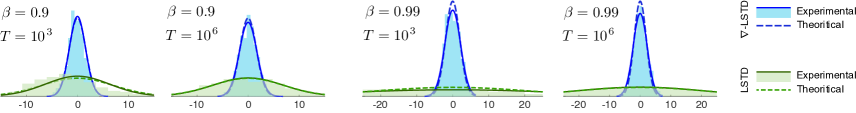
Figure 1: Histograms of $\sqrt{T}\big{(}\theta_{2}(T)-\theta^{*}_{2}\big{)}$ produced by the LSTD-learning and the $\nabla$-LSTD-learning algorithms, after $T=10^{3}$ and $T=10^{6}$ iterations. The experimental bell-curves are those obtained using histfit in Matlab using parameter estimates from multiple runs of each algorithm. Computation of the theoretical variance is obtained in Appendix C. – see (59), and the discussion that follows.

To obtain the required representation for $b$, recall that $\zeta(t)\equiv\varphi(t)$, where the former is defined in (47) and the latter in the recursion of Algorithm 2. Applying Lemma 3.6, it follows that the vector $b$ of the $\nabla$-LSTD(1) algorithm (46) coincides with the vector $b$ of $\nabla$-LSTD algorithm (42).     $\Box$

5 Numerical Results

Collected together here are results from several numerical experiments, which illustrate the general theory of the previous sections and also suggest possible extensions.

Since, under general conditions, all estimates considered obey a central limit theorem [42], we use the asymptotic variance to be the primary figure of merit in evaluating performance. The relevant variances are estimated by collecting data from many independent runs of each algorithm.

Specifically, we show comparisons between the performance achieved by LSTD, $\nabla$-LSTD, LSTD($\lambda$) and the $\nabla$-LSTD($\lambda$) algorithms. In examples where there is regeneration (the Markov chain $X$ visits some state infinitely often), we replace the LSTD algorithm with the regenerative LSTD algorithm of [3, 26]. The regenerative algorithm is found to have reduced variance in these experiments.

The standard TD($\lambda$) algorithm was also considered, but in all examples its variance was found to be several orders of magnitude greater than alternatives. The matrix-gain variant with minimal asymptotic variance is precisely LSTD($\lambda$) [32, 23]. This was found to have better performance, and was therefore used for comparisons; the reader is referred to Section 2.4 of [23] for details on the relationship between TD($\lambda$) and LSTD($\lambda$) algorithms, and their asymptotic variances.

We also consider two extensions of $\nabla$-LSTD for a specific example: The approximation of the relative value function for the speed-scaling model of [44]. First, for this reflected process evolving on ${\mathbb{R}}_{+}$, it is shown that the sensitivity process $\bfSens$ can be defined, subject to conditions on the dynamics near the boundary. Second, the algorithm is tested in a discrete state space setting. There is no apparent justification for this approach, but it performs remarkably well in simulations.

5.1 Linear model

A scalar linear model offers perhaps the clearest illustration of the performance of the $\nabla$-LSTD-learning algorithm, demonstrating its superior convergence rate compared to the standard LSTD algorithm.

Consider the scalar linear process

$$X(t+1)=aX(t)+N(t+1),\quad t\geq 1,$$

where $a\in(0,1)$ is a constant and $N$ is i.i.d. ${\cal N}(0,1)$. The cost function is taken to be quadratic, $c(x)=x^{2}$, and for the basis of the approximating function class is chosen as $\psi(x)=(1,x^{2})^{\hbox{\tiny\it T}}$. The true value function $h_{\beta}$ turns out to also be quadratic and symmetric, which means that it can be expressed exactly in terms of $\psi$, as $h_{\beta}=h_{\beta}^{\theta^{*}}$, with,

$$h_{\beta}^{\theta^{*}}(x)=\sum_{j}\theta_{j}\psi_{j}(x)=\theta_{1}^{*}+\theta_{2}^{*}x^{2},$$

for appropriate $\theta^{*}\in{\mathbb{R}}^{2}$; cf. (7). The constant term, $\theta_{1}^{*}$, can be estimated as $\kappa(\theta)$ using (32) in the $\nabla$-LSTD algorithm. Therefore, the interesting part of the problem is to estimate the optimal value of the second parameter, $\theta_{2}^{*}$.

For this linear model, the first recursion for the $\nabla$-LSTD Algorithm 2 becomes,

$$\varphi(t)=\beta a\varphi(t-1)+\nabla\psi(X(t)),$$ (48)

while in the LSTD Algorithm 1,

$$\varphi(t)=\beta\varphi(t-1)+\psi(X(t)).$$ (49)

Although both of these algorithms are consistent, there are two differences which immediately suggest that the asymptotic variance of $\nabla$-LSTD should be much smaller than that of LSTD. First, the additional discounting factor $a$ appearing in (48), but absent in (49), is the reason why the asymptotic variance of the $\nabla$-LSTD is bounded over $0<\beta<1$, whereas that of the standard LSTD grows without bound as $\beta\to 1$. Second, the gradient reduces the growth rate of each function of $x$; in this case, reducing the quadratic growth of $c$ and $\psi$ to the linear growth of their derivatives.

In the numerical experiments surveyed here we use $a=0.7$, and two different discounting factors: $\beta=0.9$, and $\beta=0.99$. The optimal parameters can be computed explicitly, giving $\theta^{*}=(16.1,1.79)^{\hbox{\tiny\it T}}$ when $\beta=0.9$, and $\theta^{*}=(192.27,1.9421)^{\hbox{\tiny\it T}}$ when $\beta=0.99$. The histogram of the estimated value of $\theta_{2}$ was computed based on 1000 repetitions of the same experiment, where the output of each algorithm was recorded after $T=10^{3}$ and after $T=10^{6}$ iterations. The results are shown in Figure 1.

With $\beta=0.9$ it was found that the variance of $\theta_{2}$ using the standard LSTD algorithm is about ten times the variance using the $\nabla$-LSTD algorithm. Consequently, $\nabla$-LSTD-learning is about $10$ times faster than LSTD in this example. This difference in performance grows with larger $\beta$, as observed on the two histograms on the right hand side of Figure 1.

In conclusion, in contrast to the standard LSTD algorithm, the asymptotic variance of $\nabla$-LSTD in this example is bounded uniformly over $0<\beta<1$, and the algorithm can also be used to estimate the relative value function (6).

We next consider an example with non-linear dynamics.

5.2 Dynamic speed scaling

Dynamic speed scaling refers to control techniques for power management in computer systems. The goal is to control the processing speed so as to optimally balance energy and delay costs; this can be done by reducing (or increasing) the processor speed at times when the workload is small (respectively, large). For our present purposes, speed scaling is a simple stochastic control problem, namely, a single-server queue with controllable service rate.

This example was considered in [44] with the goal of minimizing the average cost (4). Approximate policy iteration was used to obtain the optimal control policy, and a regenerative form of the LSTD-learning was used to provide an approximate relative value function $h$ at each iteration.

The underlying discrete-time Markov decision process model is as follows: At each time $t$, the state $X(t)$ is the (not necessarily integer valued) queue length, which can also be interpreted more generally as the size of the workload in the system; $N(t)\geq 0$ is number of job arrivals; and $U(t)$ is the service completion at time $t$, which is subject to the constraint $0\leq U(t)\leq X(t)$. The evolution equation is the controlled random walk:

$$X(t+1)=X(t)-U(t)+N(t+1)\,,\quad t\geq 0.$$ (50)

Under the assumption that $N$ is i.i.d.  and that ${\mbox{\boldmath$U$}}=\{U(t)\}$ is obtained using a state feedback policy, $U(t)=\text{f}(X(t))$, the controlled model is a Markov chain of the form (1).

In the experiments that follow in Sections 5.2.1 and 5.2.2 we consider the problem of approximating the relative value function $h$, for a fixed state feedback policy f, so $\beta=1$ throughout. We consider the cost function $c(x,u)=x+u^{2}/2$, and feedback law f given by,

$$\text{f}(x)=\min\{x,1+\varepsilon\sqrt{x}\},\quad x\in{\mathbb{R}},$$ (51)

with $\varepsilon>0$. This is similar in form to the optimal average-cost policy computed in [44], where it was shown that the value function is well-approximated by the function $h^{\theta}(x)=\theta^{\hbox{\tiny\it T}}\psi(x)$ for some $\theta\in{\mathbb{R}}^{2}_{+}$, and $\psi(x)=(x^{3/2},x)^{\hbox{\tiny\it T}}$. As in the linear example, the gradient $\nabla\psi(x)=(\frac{3}{2}x^{1/2},1)^{\hbox{\tiny\it T}}$ has slower growth as a function of $x$.

On a more technical note, we observe that implementation of the $\nabla$-LSTD algorithms requires attention to the boundary of the state space: The sensitivity process $\bfSens$ defined in (21) requires that the state space be open, and that the dynamics are smooth. Both of these assumptions are violated in this example. However, with $X(0)=x$, we do have a representation for the right derivative, ${\cal S}(t)\mathbin{:=}\partial^{+}X(t)/\partial x,$ which evolves according to the recursive equation,

$${\cal S}(t+1)={\cal A}(t+1){\cal S}(t)=\big{[}1-{\mathchoice{\genfrac{}{}{}{1}{d^{+}}{dx}}{\genfrac{}{}{}{1}{d^{+}}{dx}}{\genfrac{}{}{}{3}{d^{+}}{dx}}{\genfrac{}{}{}{3}{d^{+}}{dx}}}\text{f}\,(X(t))\big{]}{\cal S}(t),$$ (52)

where the ‘$+$’ again denotes right derivative. Therefore, we adopt the convention,

$${\cal A}(t+1)=1-{\mathchoice{\genfrac{}{}{}{1}{d^{+}}{dx}}{\genfrac{}{}{}{1}{d^{+}}{dx}}{\genfrac{}{}{}{3}{d^{+}}{dx}}{\genfrac{}{}{}{3}{d^{+}}{dx}}}\text{f}\,(X(t))$$ (53)

We begin with the case in which the marginal of $N$ is exponential. In this case the right derivatives and ordinary derivatives coincide a.e. The regenerative LSTD algorithm used in [44] is not applicable in this case because there is no state that is visited infinitely often with probability one. We therefore restrict our comparisons to the LSTD($\lambda$) algorithms.

5.2.1 Exponential arrivals

Suppose the $N(t)$ are i.i.d. Exponential$(1)$ random variables, and that $X$ evolves on ${\mathbb{R}}_{+}$ according to (50) and (51). The derivatives ${\cal A}(t)$ in (53) become,

$${\cal A}(t+1)=\hbox{\rm\large{1}}\{X(t)>\bar{\varepsilon}\}\bigl{[}1-{\mathchoice{\genfrac{}{}{}{1}{1}{2}}{\genfrac{}{}{}{1}{1}{2}}{\genfrac{}{}{}{3}{1}{2}}{\genfrac{}{}{}{3}{1}{2}}}\varepsilon X(t)^{-1/2}\bigr{]}\,,$$ (54)

where $\bar{\varepsilon}={\mathchoice{\genfrac{}{}{}{1}{1}{2}}{\genfrac{}{}{}{1}{1}{2}}{\genfrac{}{}{}{3}{1}{2}}{\genfrac{}{}{}{3}{1}{2}}}(\varepsilon+\sqrt{\varepsilon^{2}+4})$ and 1 is the indicator function.

For the implementation of the $\nabla$-LSTD Algorithm 2, we note that the recursion for $\varphi$,

$$\varphi(t+1)={\cal A}(t+1)\varphi(t)+\nabla\psi(X(t+1)),$$ (55)

regenerates: Based on (54), $\varphi(t+1)=\nabla\psi(X(t+1))$ when $X(t)\leq\bar{\varepsilon}$. The second recursion in Algorithm 2 becomes,

$$b(t+1)=b(t)+\alpha_{t+1}\bigl{(}-b(t)+\nabla c(X(t+1))\varphi(t+1)\bigr{)},$$

in which,

$$\nabla c(X(t)) =1+\text{f}(X(t))\nabla\text{f}(X(t)),$$ (56)

$$\textstyle\nabla\text{f}(X(t)) =\hbox{\rm\large{1}}\{X(t)\leq\text{f}(X(t))\}+\frac{\varepsilon}{2}\frac{1}{\sqrt{X(t)}}\hbox{\rm\large{1}}\{X(t)>\bar{\varepsilon}\}.$$

Implementation of the $\nabla$-LSTD($\lambda$) Algorithm 4 uses similar modifications, with $\{{\cal A}(t)\}$ and $\{\nabla c(X(t))\}$ obtained using (54) and (56).

Various forms of the TD($\lambda$) algorithms with $\lambda\in[0,1)$ were implemented for comparison, but as reasoned in Section 1, all of them appeared to have infinite asymptotic variance. Implementation of the LSTD($\lambda$) algorithm resulted in improved performance. Since this is an average-cost problem, Algorithm 3 must be modified slightly [6, 32, 3]:

Algorithm 5 LSTD($\lambda$) algorithm for average cost

1:Initial $\eta(0)\in{\mathbb{R}}^{+}$, $b(0),\varphi(0),\eta_{\psi}(0)\in{\mathbb{R}}^{d}$, $M(0)$ $d\times d$ positive definite, and $t=1$

2:repeat

3:     $\eta(t)=(1-\alpha_{t})\eta(t-1)+\alpha_{t}c(X(t))$

4:     $\eta_{\psi}(t)=(1-\alpha_{t})\eta_{\psi}(t-1)+\alpha_{t}\psi(X(t))$

5:     $\widetilde{\psi}(t)\mathbin{:=}\psi(X(t))-\eta_{\psi}(t)$

6:     $\zeta(t)=\lambda\zeta(t-1)+\widetilde{\psi}(X(t))$;

7:     $b(t)=(1-\alpha_{t})b(t-1)+\alpha_{t}\zeta(t)\big{(}c(X(t))-\eta(t)\big{)}$;

8:     $M(t)=(1-\alpha_{t})M(t-1)$

9:$+\alpha_{t}\zeta(t)\bigl{[}\widetilde{\psi}(X(t))-\widetilde{\psi}(X(t+1))\bigr{]}^{\hbox{\tiny\it T}}$;

10:     $t=t+1$

11:until $t\geq T$

12:$\theta=M^{-1}(T)b(T)$

Other than taking $\beta=1$, the main difference between Algorithms 3 and 5 is that we have replaced the cost function $c(X(t))$ with its centered version, $c(X(t))-\eta(t)$, where $\eta(t)$ is the estimate of the average cost after $t$ iterations. While this is standard for average cost problems, we have similarly replaced the basis function $\psi$ with $\widetilde{\psi}$ to restrict the growth rate of the eligibility vector $\zeta(t)$, which in turn reduces the variance of the estimates ${\mbox{\boldmath$\theta$}}=\{\theta(t)\}$. This is justified because the approximate value functions $h^{\theta}_{a}=\theta^{\hbox{\tiny\it T}}\widetilde{\psi}$ differs from $h^{\theta}_{b}=\theta^{\hbox{\tiny\it T}}\psi$ only by a constant term, and the relative value function is unique only up to additive constants. Experiments where $\psi$ was used instead of $\widetilde{\psi}$ resulted in worse performance.

Figure 2 shows the histogram of the estimates for $\theta_{1}$ and $\theta_{2}$ obtained using $\nabla$-LSTD-learning, LSTD($0$)-learning, and $\nabla$-LSTD($\lambda$)-learning, $\lambda=0$ and $0.5$, after $T=10^{5}$ time steps.

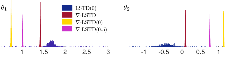
Figure 2: Histograms of the parameter estimates obtained using the LSTD and $\nabla$-LSTD algorithms after $T=10^{5}$ iterations, under the stationary policy (51) with $\varepsilon=0.5$; $N$ is i.i.d. exponential.

As noted earlier in Section 4.3, we observe that, as expected, different values of $\lambda$ lead to different parameter estimates $\theta^{*}(\lambda)$, for both the LSTD($\lambda$) and the $\nabla$-LSTD($\lambda$) classes of algorithms.

5.2.2 Geometric arrivals

In [44], the authors consider a discrete state space, with $N(t)$ geometrically distributed on an integer lattice $\{0,\Delta,2\Delta,\dots\}$, $\Delta>0$. In this case, the theory developed for the $\nabla$-LSTD algorithm does not fit the model since we have no convenient representation of a sensitivity process. Nevertheless, the algorithm can be run by replacing gradients with ratios of differences. In particular, in implementing the algorithm we substitute the definition (54) with,

$${\cal A}(t)=1-[\text{f}(X(t)+\Delta)-\text{f}(X(t))]/\Delta,$$

and $\nabla c$ is approximated similarly. For the distribution of $N(t)$ we take, ${\sf P}(N(t)=n\Delta)=(1-p_{A})^{n}p_{A}$; the values $p_{A}=0.04$ and $\Delta=1/24$ were chosen, so that ${\sf E}[N(t)]=1$.

The sequence of steps followed in the regenerative LSTD-learning algorithm are similar to Algorithm 1 [44, 3]:

Algorithm 6 Regenerative LSTD algorithm for average cost

1:Initial $\eta(0)\in{\mathbb{R}}^{+}$, $b(0),\varphi(0),\eta_{\psi}(0)\in{\mathbb{R}}^{d}$, $M(0)$ $d\times d$ positive definite, and $t=1$

2:repeat

3:     $\eta(t)=(1-\alpha_{t})\eta(t-1)+\alpha_{t}c(X(t))$

4:     $\eta_{\psi}(t)=(1-\alpha_{t})\eta_{\psi}(t-1)+\alpha_{t}\psi(X(t))$

5:     $\widetilde{\psi}(t)\mathbin{:=}\psi(X(t))-\eta_{\psi}(t)$

6:     $\varphi(t)=\hbox{\rm\large{1}}\{X(t-1)\neq 0\}\varphi(t-1)+\widetilde{\psi}(X(t))$;

7:     $b(t)=(1-\alpha_{t})b(t-1)+\alpha_{t}\varphi(t)\big{(}c(X(t))-\eta(t)\big{)}$;

8:     $M(t)=(1-\alpha_{t})M(t-1)+\alpha_{t}\big{(}\widetilde{\psi}(X(t))\widetilde{\psi}^{\hbox{\tiny\it T}}(X(t))\big{)}$;

9:     $t=t+1$

10:until $t\geq T$

11:$\theta=M^{-1}(T)b(T)$

The eligibility vector $\varphi(t)$ regenerates (i.e., resets to $0$) every time the queue empties. The regenerative LSTD($\lambda$) algorithm is obtained by making similar modifications, namely, replacing Line $5$ of Algorithm 5 with:

$$\zeta(t)=\hbox{\rm\large{1}}\{X(t-1)\neq 0\}\lambda\zeta(t-1)+\widetilde{\psi}(X(t)).$$

Figure 3 shows the histogram of $\theta(T)$ obtained using the regenerative LSTD, LSTD($0$), $\nabla$-LSTD, $\nabla$-LSTD($0$), and $\nabla$-LSTD($0.5$) algorithms, after $T=10^{5}$ iterations. Observe that, again, the variance of the parameters obtained using the $\nabla$-LSTD algorithms is extremely small compared to the LSTD algorithms.

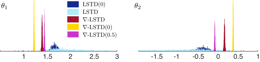
Figure 3: Histograms of the parameter estimates obtained using the LSTD and $\nabla$-LSTD algorithms after $T=10^{5}$ iterations, under the stationary policy (51) with $\varepsilon=0.5$; $N$ is i.i.d. geometric.

It is once again noticeable in Figure 3 that, as before in the results shown in Figure 2, different values for $\lambda$ lead to different parameter estimates. To compare performance, the relative Bellman error was computed:

$${\cal E}_{B}(x)=[P-I]h(x)+c(x)-\eta(T),$$

where $P$ of course depends on the policy f, $h={\bar{\theta}}^{\hbox{\tiny\it T}}\psi$, where ${\bar{\theta}}$ is the mean of the $10^{3}$ parameter estimates obtained for each of the different algorithms, and $\eta(T)$ denotes the estimate of the average cost $\eta$ using $T=10^{5}$ samples. Figure 4 shows plots of ${\cal E}_{B}(x)$ for each of the five algorithms, for typical values of $\theta(T)$, with $T=10^{3}$, $10^{4}$ and $10^{5}$. Once again, the feedback policy (51) was used, with $\varepsilon=0.5$.

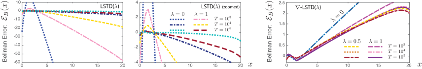
Figure 4: Bellman error corresponding to the estimates of $h$ using LSTD algorithms (left) and $\nabla$-LSTD algorithms (right).

The Bellman error of the $\nabla$-LSTD algorithms appears to have converged after $T=10^{3}$ iterations, and the limit is nearly zero for the range of $x$ where the stationary distribution has non-negligible mass. Achieving similar performance using the LSTD algorithms requires more than $T=10^{5}$ iterations.

6 Conclusions

The new gradient-based temporal difference learning algorithms introduced in this work prove to be excellent alternatives to the more classical TD- and LSTD-learning methods for value function approximation. In the examples considered, the algorithms show remarkable capability to reduce the variance. There are two known explanations for this:

• The magnitude of the functions that are used as inputs to the $\nabla$-LSTD algorithms are smaller compared to those in the case of LSTD algorithms; for example, if the basis functions for LSTD are polynomials of order $n$, then the basis functions for $\nabla$-LSTD will be of the order $n-1$.

• There is an additional “discounting” factor that is inherent in the $\nabla$-LSTD algorithms, due to the derivative sequence $\{{\cal A}(t)\}$. For example, in the simple linear model experiment (cf. Section 5.1), we had ${\cal A}(t)\equiv a$, for some $a<0$, and when this term multiplies the original discount factor $\beta$, it can cause a significant reduction in the growth rate of the eligibility trace.

The introduction of $\lambda$ is to further reduce variance. However, the optimal parameter vector obtained using the $\nabla$-LSTD($\lambda$) algorithm will not in general solve the minimum-norm problem (30) if $\lambda<1$. As in the case of classical LSTD($\lambda$) algorithms, one can expect a bias versus variance trade-off in choosing $\lambda$ for the $\nabla$-LSTD($\lambda$) algorithms. It is conjectured that as $\lambda\to 0$, the bias becomes larger, and perhaps the variance reduces. A bound similar to (13) is a topic of future research.

Though we only consider problems that involve ultimately estimating the value function for a fixed policy, estimating the gradient of the value function has its own applications:

State estimation. In [45], the authors are interested in estimating the gradient of the relative value function, which is useful in obtaining the innovation gain for a non-linear filter.

Control. When one is interested in optimizing the policy using policy iteration in a continuous state space setting, the gradient of the value function could be more useful than the value function, in the policy update step.

Mean-field games. As was recently emphasised in [46], “…it is not the Bellman equation that is important, but the gradient of its solution.” That is, it is the gradient of the value functions that is the critical quantity of interest in computation of solutions to mean field games. This appears to indicate that the techniques in this paper might offer computational tools for approximating solutions in this class of optimal control problems, and in particular in applications to power systems.

Perhaps the biggest drawback of the $\nabla$-LSTD algorithms is the requirement of the knowledge of ${\cal A}(t)$ defined in (23). In certain problems (such as in the queuing example discussed in Section 5.2) this information is directly available. Other applications may require a combination of system identification with the $\nabla$-LSTD algorithm.

There are many other directions in which this work can be extended. Perhaps the most interesting open question is why the algorithm is so effective even in a discrete state space setting in which there is no theory to justify its application. It will also be worth exploring algorithms analogous to $\nabla$-LSTD, which use finite-differences instead of gradients in a discrete state space setting.

We are currently considering the extension of the $\nabla$-LSTD algorithms to a continuous time setting. Though the algorithms are straightforward to obtain, the convergence theory will require extensions of the theory of [28].

Finally, it will be interesting to see how the techniques developed here could be used to estimate the gradient of the state-action value function (either the Q-function of Watkins [47] or SARSA [48]). This will greatly simplify application to control.

Appendix A Proof of Prop. 2.2

Here we state and prove two simple technical lemmas that are needed for the proof of Prop. 2.2. Let $v$ denote the Lyapunov function in Assumption A1.

Lemma A.1.

Let $R$ denote a transition kernel that has the Feller property and satisfies, for some $B_{0}<\infty$:

$$Rv\,(x)\mathbin{:=}\int R(x,dy)v(y)\leq B_{0}v(x)\,,\quad x\in{\mathbb{R}}^{\ell}.$$

And let $Z$ be a kernel that is absolutely continuous with respect to $R$, with density $\xi\colon{\mathbb{R}}^{\ell}\times{\mathbb{R}}^{\ell}\to{\mathbb{R}}$ such that,

$$Zg\,(x)=\int R(x,dy)\xi(x,y)g(y)\,,\quad x\in{\mathbb{R}}^{\ell},$$

for any bounded measurable function $g\colon{\mathbb{R}}^{\ell}\to{\mathbb{R}}$.

If the density is continuous and for some $\delta\in(0,1)$,

$$B_{\xi}\mathbin{:=}\sup_{x,y}\frac{|\xi(x,y)|}{v^{\delta}(y)}<\infty,$$

then $Z$ has the Feller property: $Zg$ is continuous whenever $g$ is bounded and continuous.

Proof.

The proof is based on a truncation argument: Consider the sequence of closed sets,

$$S_{n}=\{x\in{\mathbb{R}}^{\ell}:v(x)\leq n\},\quad\,n\geq 1.$$

Take any sequence of continuous functions $\{{\mathchoice{\mathord{\raisebox{1.5pt}{\scalebox{1.25}{$\chi$}}}}{\mathord{\raisebox{1.5pt}{\scalebox{1.25}{$\chi$}}}}{\mathord{\raisebox{1.0pt}{\scalebox{0.75}{$\chi$}}}}{\mathord{\raisebox{0.8pt}{\scalebox{0.6}{$\chi$}}}}}_{n}:n\geq 1\}$ satisfying $0\leq{\mathchoice{\mathord{\raisebox{1.5pt}{\scalebox{1.25}{$\chi$}}}}{\mathord{\raisebox{1.5pt}{\scalebox{1.25}{$\chi$}}}}{\mathord{\raisebox{1.0pt}{\scalebox{0.75}{$\chi$}}}}{\mathord{\raisebox{0.8pt}{\scalebox{0.6}{$\chi$}}}}}_{n}(x)\leq 1$ for all $x$, ${\mathchoice{\mathord{\raisebox{1.5pt}{\scalebox{1.25}{$\chi$}}}}{\mathord{\raisebox{1.5pt}{\scalebox{1.25}{$\chi$}}}}{\mathord{\raisebox{1.0pt}{\scalebox{0.75}{$\chi$}}}}{\mathord{\raisebox{0.8pt}{\scalebox{0.6}{$\chi$}}}}}_{n}(x)=1$ on $S_{n}$, and ${\mathchoice{\mathord{\raisebox{1.5pt}{\scalebox{1.25}{$\chi$}}}}{\mathord{\raisebox{1.5pt}{\scalebox{1.25}{$\chi$}}}}{\mathord{\raisebox{1.0pt}{\scalebox{0.75}{$\chi$}}}}{\mathord{\raisebox{0.8pt}{\scalebox{0.6}{$\chi$}}}}}_{n}(x)=0$ on $S_{n+1}^{c}$. Hence ${\mathchoice{\mathord{\raisebox{1.5pt}{\scalebox{1.25}{$\chi$}}}}{\mathord{\raisebox{1.5pt}{\scalebox{1.25}{$\chi$}}}}{\mathord{\raisebox{1.0pt}{\scalebox{0.75}{$\chi$}}}}{\mathord{\raisebox{0.8pt}{\scalebox{0.6}{$\chi$}}}}}_{n}$ is a continuous approximation to the indicator on $S_{n}$.

Denote $g_{n}=g{\mathchoice{\mathord{\raisebox{1.5pt}{\scalebox{1.25}{$\chi$}}}}{\mathord{\raisebox{1.5pt}{\scalebox{1.25}{$\chi$}}}}{\mathord{\raisebox{1.0pt}{\scalebox{0.75}{$\chi$}}}}{\mathord{\raisebox{0.8pt}{\scalebox{0.6}{$\chi$}}}}}_{n}$ for a given bounded and continuous function $g$. The function $Zg_{n}$ is continuous because $\xi(x,y)g_{n}(y)$ is bounded and continuous. It remains to show that $Zg=\lim_{n\to\infty}Zg_{n}$, and that the convergence is uniform on compact sets.

Under the assumptions of the lemma, for each $x$,

$$|Zg\,(x)-Zg_{n}\,(x)| \leq\|g\|_{\infty}\int R(x,dy)[1-{\mathchoice{\mathord{\raisebox{1.5pt}{\scalebox{1.25}{$\chi$}}}}{\mathord{\raisebox{1.5pt}{\scalebox{1.25}{$\chi$}}}}{\mathord{\raisebox{1.0pt}{\scalebox{0.75}{$\chi$}}}}{\mathord{\raisebox{0.8pt}{\scalebox{0.6}{$\chi$}}}}}_{n}(y)]|\xi(x,y)|$$

$$\leq B_{\xi}\|g\|_{\infty}\int_{S_{n}^{c}}R(x,dy)v^{\delta}(y).$$

Since $v(y)>n$ on $S_{n}^{c}$, this gives, for all $x$,

$$|Zg\,(x)-Zg_{n}\,(x)|\leq\frac{1}{n^{1-\delta}}B_{0}B_{\xi}\|g\|_{\infty}v(x).$$

It follows that $Zg_{n}\to Zg$ uniformly on compact sets, since $v$ is assumed to be continuous.     $\Box$

Lemma A.2.

Subject to Assumptions A1 and A2,

• $P^{t}f$ is continuous if $|f|^{2}\in L_{\infty}^{v}$ and $f$ is continuous.

• The vector-valued function $Q^{t}\nabla f$ is continuous, provided $\nabla f$ is continuous, $|f|^{2}\in L_{\infty}^{v}$, and $\|\nabla f\|_{2}^{2}\in L_{\infty}^{v}$.

Proof.

Both parts follow from Lemma A.1, with $R=P^{t}$. The bound $P^{t}v\leq B_{0}v$ holds under A1, and in fact the constant $B_{0}$ can be chosen independent of $t$.

For part (i), choose $\xi(x,y)=f(y)$. The Feller property for the kernel $Z$ defined in Lemma A.1 implies in particular that $Zg$ is continuous when $g\equiv 1$. $Zg=P^{t}f$ in this special case. For part (ii), observe that each $Q^{t}_{i,j}$ $1\leq i,j\leq\ell$, admits a continuous and bounded density by its definition, cf. (22), (26):

$$Q^{t}_{i,j}(x,dy)=P^{t}(x,dy)q^{t}_{i,j}(x,y).$$

So, we have for each $i$ and $x$,

$$[Q^{t}\nabla f\,(x)]_{i}=\sum_{j}\int P^{t}(x,dy)q^{t}_{i,j}(x,y)[\nabla f(y)]_{j}\,.$$

Fix $i,j$ and let $\xi(x,y):=q^{t}_{i,j}(x,y)[\nabla f(y)]_{j}$. Then Lemma A.1 implies that the $(i,j)$-term in the last sum, $\int P^{t}(x,dy)q^{t}_{i,j}(x,y)[\nabla f(y)]_{j}$, is continuous in $x$.     $\Box$

Appendix B Proof of Lemma 3.6

The following shift-operator on sample space is defined for a stationary version of $X$: For a random variable of the form,

$$Z=F(X(r),N(r),\dots,X(s),N(s))\,,\quad\text{with $r\leq s$,}$$

we denote, for any integer $k$,

$$\Theta^{k}Z=F(X(r+k),N(r+k),\dots,X(s+k),N(s+k)).$$

Consequently, viewing ${\cal S}(t)$ as a function of ${\cal A}(1),\ldots,{\cal A}(t)$ as in the evolution equation (22), we have:

$$\Theta^{k}{\cal S}(t)={\cal A}(t+k)\cdots{\cal A}(2+k){\cal A}(1+k).$$ (57)

The representation (20) for $\nabla h_{\beta}$ is valid under Assumption A3, by Lemma 3.3. Using this and (22) gives the first representation in (42):

$$b^{\hbox{\tiny\it T}} =\int{\sf E}_{x}\big{[}(\Omega_{\beta}\nabla c(x))^{\hbox{\tiny\it T}}\nabla\psi(x)\big{]}\pi(dx)$$ (58)

$$=\sum_{t=0}^{\infty}\beta^{t}\int{\sf E}_{x}\big{[}({\cal S}^{\hbox{\tiny\it T}}(t)\nabla c(x))^{\hbox{\tiny\it T}}\nabla\psi(x)\big{]}\pi(dx)$$

$$=\sum_{t=0}^{\infty}\beta^{t}{\sf E}\bigl{[}\bigl{(}{\cal S}^{\hbox{\tiny\it T}}(t)\nabla c(X(t))\bigr{)}^{\hbox{\tiny\it T}}\nabla\psi(X(0))\bigr{]}\,.$$

Stationarity implies that for any $t,k\in\mathbb{Z}$,

$${\sf E}\Bigl{[}\Bigl{(} {\cal S}^{\hbox{\tiny\it T}}(t)\nabla c(X(t))\Bigr{)}^{\hbox{\tiny\it T}}\nabla\psi(X(0))\Bigr{]}$$

$$={\sf E}\Bigl{[}\Bigl{(}[\Theta^{k}{\cal S}^{\hbox{\tiny\it T}}(t)]\nabla c(X(t+k))\Bigr{)}^{\hbox{\tiny\it T}}\nabla\psi(X(k))\Bigr{]}\,.$$

Setting $k=-t$, the first representation in (42) becomes:

$$b^{\hbox{\tiny\it T}} =\sum_{t=0}^{\infty}\beta^{t}{\sf E}\Bigl{[}\big{(}\nabla c(X(0))\big{)}^{\hbox{\tiny\it T}}\big{(}\Theta^{-t}{\cal S}(t)\big{)}\nabla\psi(X(-t))\Bigr{]}$$

$$={\sf E}\Bigl{[}\big{(}\nabla c(X(0))\big{)}^{\hbox{\tiny\it T}}\Bigl{(}\sum_{t=0}^{\infty}\beta^{t}\big{(}\Theta^{-t}{\cal S}(t)\big{)}\nabla\psi(X(-t))\Bigr{)}\Bigr{]}\,,$$

where last equality is obtained under Assumption A3 by applying Fubini’s theorem. This combined with (41) completes the proof.     $\Box$

Appendix C Variance Analysis of $\nabla$-LSTD($\lambda$) Algorithms

As in the case of the classical LSTD($\lambda$) algorithms, the $\nabla$-LSTD($\lambda$) algorithms also belong to a more general class of root-finding algorithms known as stochastic approximation (SA). Following the theory for variance analysis of linear SA recursions, under slightly stronger conditions than Prop. 3.5 and Prop. 4.3, the asymptotic variance of the $\nabla$-LSTD($\lambda$) algorithm is given by the following expression [42, 22, 23]:

$$\Sigma_{\theta} \mathbin{:=}\lim_{T\to\infty}T{\sf E}\big{[}\big{(}\theta(T)-\theta^{*}\big{)}\big{(}\theta(T)-\theta^{*}\big{)}^{\hbox{\tiny\it T}}\big{]}$$ (59)

$$=M^{-1}\Sigma_{\Delta}\big{(}M^{-1}\big{)}^{\hbox{\tiny\it T}}$$

where, the matrix $M$ is defined in (45), and the “noise covariance matrix” is defined as follows: define

$$\Delta(t)\mathbin{:=}\widetilde{M}(t)\theta^{*}+\widetilde{b}(t)$$ (60)

where (with the quantities defined in Algorithm 2),

$$\widetilde{M}(t) \mathbin{:=}M-\bigl{[}\nabla\psi(X(t))-\beta{\cal A}^{\hbox{\tiny\it T}}(t+1)\nabla\psi(X(t+1))\bigr{]}^{\hbox{\tiny\it T}}\zeta(t)$$ (61)

$$\widetilde{b}(t) \mathbin{:=}b-\zeta^{\hbox{\tiny\it T}}(t)\nabla c(X(t))$$

with $b$ is defined in (46), $\theta^{*}=M^{-1}b$, and all stochastic processes are assumed stationary. The noise covariance matrix is then expressed by the two equivalent formula:

$$\Sigma_{\Delta}=\lim_{T\to\infty}\frac{1}{T}{\sf E}\big{[}S(T)S(T)^{\hbox{\tiny\it T}}\big{]}=\sum_{t=-\infty}^{\infty}R(t)$$ (62)

where

$$R(t)={\sf E}\big{[}\big{(}\widetilde{M}(t)\theta^{*}-\widetilde{b}(t)\big{)}\big{(}\widetilde{M}(0)\theta^{*}-\widetilde{b}(0)\big{)}^{\hbox{\tiny\it T}}\big{]},\,\quad t\geq 0\,,$$ (63)

with $R(-t)=R(t)^{\hbox{\tiny\it T}}$, and $S(T)=\sum_{t=0}^{T-1}\Delta(t)$.

An asymptotic variance formula for LSTD($\lambda$) algorithms can be obtained in a straightforward manner, using the definitions of $M$, $M(t)$, $b$, and $b(t)$ as in Algorithm 1 and Prop. 3.1.

In the following, we show how these expressions can be used to calculate the asymptotic variance of the two algorithms when applied to the simple linear model described in Section 5.1, and how the algorithms compare with each other with respect to this quantity.

Appendix D Asymptotic Variance for the Linear Model

Consider the application of $\nabla$-LSTD and LSTD algorithms to estimate the value function for the linear model that is analyzed in Section 5.1:

$$X(t+1)=aX(t)+N(t+1),\quad t\geq 1,$$ (64)

with the cost function defined to be a quadratic: $c(x)=x^{2}$.

The one dimensional basis function for $\nabla$-LSTD is given by $\nabla\psi(x)=2x$, so that the estimate of the value function is $\nabla h^{\theta}_{\beta}(x)=2\theta x$. In this case, $M$ and $b$ are scalar quantities, and $\mbox{\boldmath$\varphi$}\equiv{\mathchoice{\mbox{\boldmath$\zeta$}}{\mbox{\boldmath$\zeta$}}{\mbox{\boldmath$\scriptstyle\zeta$}}{\mbox{\boldmath$\scriptscriptstyle\zeta$}}}$ is a scalar sequence:

$$M=4{\sf E}[X^{2}(t)]\qquad b=2{\sf E}[X(t)\varphi(t)]$$

with $\varphi(t)$ defined in (48), and expectations in steady state.

Using the fact that $M\theta^{*}=b$, the auto-correlation function $R(t)$ defined in (63) is given by:

$$R(t) \!=\!{\sf E}\big{[}\big{(}4\theta^{*}X^{2}(t)-2X(t)\varphi(t)\big{)}(4\theta^{*}X^{2}(0)-2X(0)\varphi(0)\big{)}\big{]}$$

In the case $\{N(t):t\geq 1\}$ is i.i.d Gaussian with mean $0$ and variance $\sigma_{N}^{2}$, using (64), it can be shown that the above expression simplifies to:

$$R(t)= \big{(}(\theta^{*})^{2}+4-4\theta^{*}\big{)}{\sf E}\big{[}X^{2}(t)X^{2}(0)\big{]}$$ (65)

$$-2\theta^{*}a\beta\sum_{s=0}^{t-1}(a\beta)^{s}a^{t-s}{\sf E}\big{[}X^{2}(s)X^{2}(0)\big{]}$$

where, for each $t\geq 1$:

$${\sf E}[X^{2}(t)X^{2}(0)]=a^{2t}{\sf E}[X^{4}(t)]+\big{(}\sum_{s=0}^{t-1}a^{2s}\big{)}\sigma_{N}^{2}{\sf E}[X^{2}(t)]$$ (66)

and the steady state expectations are given by:

$${\sf E}[X^{2}(t)]\mathbin{:=}\frac{\sigma_{N}^{2}}{1-\alpha^{2}}\hskip 14.45377pt{\sf E}[X^{4}(t)]\mathbin{:=}\frac{\sigma_{N}^{2}}{1-\alpha^{4}}\Big{(}\frac{6}{1-\alpha^{2}}+3\Big{)}$$ (67)

The noise covariance $\Sigma_{\Delta}$ is then obtained using the second definition in (62). The plots for theoretical values of the variance $\Sigma_{\theta}$ in Figure 1 is obtained using this expression.

Similarly, for the LSTD($\lambda$) algorithm, since $\psi(x)=(1,\,x^{2})^{\hbox{\tiny\it T}}$, we have

$$M={\sf E}\begin{bmatrix}1&X^{2}(t)\\ X^{2}(t)&X^{4}(t)\end{bmatrix}\qquad b={\sf E}\big{[}X^{2}(t)\varphi(t)\big{]}$$

with $\varphi(t)$ recursively defined in (49). The auto-correlation can then be obtained using (63), where:

$$\widetilde{M}(t) \mathbin{:=}M-\psi(X(t))\psi^{\hbox{\tiny\it T}}(X(t))$$ (68)

$$\widetilde{b}(t) \mathbin{:=}b-\varphi(t)c(X(t))$$

and $\theta^{*}=M^{-1}b$. However, the precise expression for $R(t)$ becomes much more complicated than the one obtained in (65), since it involves calculation of moments up to eighth order.

An alternative way to obtain a theoretical formula for $\Sigma_{\Delta}$ is using the first definition in (62). For fixed $T$ large enough, one can approximately obtain $\Sigma_{\Delta}$ by estimating the expectation in (62) using Monte-Carlo:

$${\sf E}[S(T)S(T)^{\hbox{\tiny\it T}}]\approx\frac{1}{N}\sum_{i=0}^{N}S^{(i)}(T)\big{(}S^{(i)}(T)\big{)}^{\hbox{\tiny\it T}}\,,$$

The plots for theoretical values of the variance $\Sigma_{\theta}$ in Figure 1 were obtained using this approximation.

References

- [1] A. Devraj and S. Meyn, “Differential TD learning for value function approximation,” in Decision and Control (CDC), 2016 IEEE 55th Conference on. IEEE, 2016, pp. 6347–6354.
- [2] D. Bertsekas and J. N. Tsitsiklis, Neuro-Dynamic Programming. Cambridge, Mass: Atena Scientific, 1996.
- [3] S. P. Meyn, Control Techniques for Complex Networks. Cambridge University Press, 2007, pre-publication edition available online.
- [4] S. Chen, A. M. Devraj, A. Bušić, and S. Meyn, “Explicit mean-square error bounds for Monte-Carlo and linear stochastic approximation,” arXiv preprint arXiv:2002.02584, and to appear AISTATS, 2020.
- [5] A. M. Devraj, A. Bušić, and S. Meyn. Fundamental design principles for reinforcement learning algorithms. In Handbook on Reinforcement Learning and Control. Springer, 2020.
- [6] J. N. Tsitsiklis and B. V. Roy, “Average cost temporal-difference learning,” Automatica, vol. 35, no. 11, pp. 1799 – 1808, 1999.
- [7] D. Bertsekas and S. Shreve, Stochastic Optimal Control: The Discrete-Time Case. Athena Scientific, 1996.
- [8] V. R. Konda and J. N. Tsitsiklis, “On actor-critic algorithms,” SIAM J. Control Optim., vol. 42, no. 4, pp. 1143–1166 (electronic), 2003.
- [9] S. Asmussen and P. W. Glynn, Stochastic Simulation: Algorithms and Analysis, ser. Stochastic Modelling and Applied Probability. New York: Springer-Verlag, 2007, vol. 57.
- [10] S. P. Meyn and R. L. Tweedie, Markov chains and stochastic stability, 2nd ed. Cambridge: Cambridge University Press, 2009, published in the Cambridge Mathematical Library. 1993 edition online.
- [11] S. Henderson, “Variance reduction via an approximating Markov process,” Ph.D. dissertation, Stanford University, 1997.
- [12] S. G. Henderson, S. P. Meyn, and V. B. Tadić, “Performance evaluation and policy selection in multiclass networks,” Discrete Event Dynamic Systems: Theory and Applications, vol. 13, pp. 149–189, 2003, special issue on learning, optimization and decision making.
- [13] S. Kyriazopoulou-Panagiotopoulou, I. Kontoyiannis, and S. P. Meyn, “Control variates as screening functions,” in ValueTools ’08: Proceedings of the 3rd International Conference on Performance Evaluation Methodologies and Tools. ICST, Brussels, Belgium, Belgium: ICST (Institute for Computer Sciences, Social-Informatics and Telecommunications Engineering), 2008, pp. 1–9.
- [14] P. Dellaportas and I. Kontoyiannis, “Control variates for estimation based on reversible Markov chain Monte Carlo samplers,” Journal of the Royal Statistical Society. Series B (Statistical Methodology), vol. 74, no. 1, pp. 133–161, 2012.
- [15] N. Brosse, A. Durmus, S. Meyn, É. Moulines, and A. Radhakrishnan, “Diffusion approximations and control variates for MCMC,” Ann. Appl. Probab. (submitted) and arXiv, p. arXiv:1808.01665, 2019.
- [16] T. Yang, P. Mehta, and S. Meyn, “Feedback particle filter,” IEEE Trans. Automat. Control, vol. 58, no. 10, pp. 2465–2480, Oct 2013.
- [17] R. S. Laugesen, P. G. Mehta, S. P. Meyn, and M. Raginsky, “Poisson’s equation in nonlinear filtering,” SIAM J. Control Optim., vol. 53, no. 1, pp. 501–525, 2015.
- [18] A. Taghvaei and P. G. Mehta, “Gain function approximation in the feedback particle filter,” in Proc. of the IEEE Conf. on Dec. and Control, Dec 2016, pp. 5446–5452.
- [19] A. Radhakrishnan, A. Devraj, and S. Meyn, “Learning techniques for feedback particle filter design,” in Proc. of the IEEE Conf. on Dec. and Control, Dec 2016, pp. 5453–5459.
- [20] A. Radhakrishnan and S. Meyn, “Feedback particle filter design using a differential-loss Reproducing Kernel Hilbert Space,” in Proc. of the American Control Conf., June 2018, pp. 329–336.
- [21] R. Sutton and A. Barto, Reinforcement Learning: An Introduction. Cambridge, MA: MIT Press.
- [22] V. S. Borkar, Stochastic Approximation: A Dynamical Systems Viewpoint. Delhi, India and Cambridge, UK: Hindustan Book Agency and Cambridge University Press (jointly), 2008.
- [23] A. M. Devraj and S. P. Meyn, “Fastest convergence for Q-learning,” ArXiv e-prints, Jul. 2017.
- [24] ——, Q-learning with uniformly bounded variance: Large discounting is not a barrier to fast learning. arXiv, February 2020.
- [25] ——, “Zap Q-learning,” in Proceedings of the 31st International Conference on Neural Information Processing Systems, 2017.
- [26] D. Huang, W. Chen, P. Mehta, S. Meyn, and A. Surana, “Feature selection for neuro-dynamic programming,” in Reinforcement Learning and Approximate Dynamic Programming for Feedback Control, F. Lewis, Ed. Wiley, 2011.
- [27] V. V. G. Konda, “Actor-critic algorithms,” Ph.D. dissertation, Massachusetts Institute of Technology, 2002.
- [28] A. Devraj, I. Kontoyiannis, and S. Meyn, “Geometric Ergodicity in a Weighted Sobolev Space,” To appear, Annals of Probability (and arXiv e-prints), p. arXiv:1711.03652, Nov 2017.
- [29] J. N. Tsitsiklis and B. Van Roy, “An analysis of temporal-difference learning with function approximation,” IEEE Trans. Automat. Control, vol. 42, no. 5, pp. 674–690, 1997.
- [30] I. Kontoyiannis and S. P. Meyn, “Spectral theory and limit theorems for geometrically ergodic Markov processes,” Ann. Appl. Probab., vol. 13, pp. 304–362, 2003.
- [31] R. S. Sutton, “Learning to predict by the methods of temporal differences,” Mach. Learn., vol. 3, no. 1, pp. 9–44, 1988.
- [32] J. A. Boyan, “Technical update: Least-squares temporal difference learning,” Mach. Learn., vol. 49, no. 2-3, pp. 233–246, 2002.
- [33] L. Arnold and V. Wihstutz, “Lyapunov exponents: A survey,” in Lyapunov Exponents: Proceedings of a Workshop held in Bremen, November 12–15, 1984, L. Arnold and V. Wihstutz, Eds. Berlin, Heidelberg: Springer Berlin Heidelberg, 1986, pp. 1–26.
- [34] L. Gurvits, L. Lin, and S. Hanson, “Incremental learning of evaluation functions for absorbing Markov chains: New methods and theorems,” Unpublished manuscript, 1994.
- [35] T. Jaakkola, M. Jordan, and S. Singh, “Convergence of stochastic iterative dynamic programming algorithms,” in Advances in neural information processing systems, 1994, pp. 703–710.
- [36] F. Pineda, “Mean-field theory for batched TD(),” Neural Computation, vol. 9, no. 7, pp. 1403–1419, 1997.
- [37] H. Yu and D. Bertsekas, “Error bounds for approximations from projected linear equations,” Mathematics of Operations Research, vol. 35, no. 2, pp. 306–329, 2010.
- [38] D. Bertsekas, “Approximate policy iteration: A survey and some new methods,” Journal of Control Theory and Applications, vol. 9, no. 3, pp. 310–335, 2011.
- [39] C. Szepesvári, “Least squares temporal difference learning and galerkin’s method,” August 21–27th 2011, presentation at the Mini-Workshop: Mathematics of Machine Learning, Mathematisches Forschungsinstitut Oberwolfach.
- [40] ——, Algorithms for Reinforcement Learning, ser. Synthesis Lectures on Artificial Intelligence and Machine Learning. Morgan & Claypool Publishers, 2010.
- [41] J. Boyan, “Least-squares temporal difference learning,” in ICML, 1999, pp. 49–56.
- [42] H. J. Kushner and G. G. Yin, Stochastic approximation algorithms and applications, ser. Applications of Mathematics (New York). New York: Springer-Verlag, 1997, vol. 35.
- [43] V. Konda and J. Tsitsiklis, “Actor-critic algorithms,” in Advances in neural information processing systems, 2000, pp. 1008–1014.
- [44] W. Chen, D. Huang, A. A. Kulkarni, J. Unnikrishnan, Q. Zhu, P. Mehta, S. Meyn, and A. Wierman, “Approximate dynamic programming using fluid and diffusion approximations with applications to power management,” in Proc. of the 48th IEEE Conf. on Dec. and Control; held jointly with the 2009 28th Chinese Control Conference, 2009, pp. 3575–3580.
- [45] T. Yang, P. G. Mehta, and S. P. Meyn, “A mean-field control-oriented approach to particle filtering,” in Proc. of the 2011 American Control Conference (ACC), July 2011, pp. 2037–2043.
- [46] A. Bensoussan, “Machine learning and control theory (plenary lecture),” in Advances in Modelling and Control for Power Systems of the Future, Palaiseau, France, September 2018.
- [47] C. J. C. H. Watkins, “Learning from delayed rewards,” Ph.D. dissertation, King’s College, Cambridge, Cambridge, UK, 1989.
- [48] G. A. Rummery and M. Niranjan, “On-line Q-learning using connectionist systems,” Cambridge Univ., Dept. Eng., Cambridge, U.K. CUED/F-INENG/, Technical report 166, 1994.
- [49] D. Silver, G. Lever, N. Heess, T. Degris, D. Wierstra, and M. Riedmiller, “Deterministic policy gradient algorithms,” in ICML, 2014.
- [50] J. Kiefer and J. Wolfowitz, “Stochastic estimation of the maximum of a regression function,” Ann. Math. Statist., vol. 23, no. 3, pp. 462–466, 09 1952.
- [51] A. Bernstein, Y. Chen, M. Colombino, E. Dall’Anese, P. Mehta, and S. Meyn, “Quasi-stochastic approximation and off-policy reinforcement learning,” in 58th IEEE Conf. on Decision and Control, 2019.