Present address: ]Department of Physics and Astronomy, Northwestern University, Evanston, IL 60208, USA

Combined Search for a Lorentz-Violating Force in Short-Range Gravity
Varying as the Inverse Sixth Power of Distance

Abstract

Precision measurements of the inverse-square law via experiments on short-range gravity provide sensitive tests of Lorentz symmetry. A combined analysis of data from experiments at the Huazhong University of Science and Technology and Indiana University sets simultaneous limits on all 22 coefficients for Lorentz violation correcting the Newton force law as the inverse sixth power of distance. Results are consistent with no effect at the level of $10^{-12}$ m⁴.

Lorentz symmetry, the idea that physical laws are unchanged under rotations and boosts, is built into both General Relativity (GR) and the Standard Model. Although GR provides an impressive description of a wide variety of gravitational phenomena, the successful merger of gravitation and quantum physics may involve a modification of its foundational principles. This could produce observable deviations from Lorentz symmetry, emerging from a unified theory such as strings ksp .

Since no compelling evidence for Lorentz violation (LV) currently exists, model-independent searches for LV in gravity play an essential role in testing the foundations of GR. A powerful model-independent approach to describing possible low-energy signals of LV is effective field theory ak04 , which is widely adopted for experimental analyses studying Lorentz symmetry tables ; lvgrreview . In the pure-gravity limit, this approach uses a Lagrange density containing the usual Einstein-Hilbert term and a series of all observer-scalar terms involving coefficients contracted with gravitational-field LV operators of increasing mass dimension $d$.

Precision experiments testing the inverse-square law at short range provide crucial and specific probes of gravitational properties review , including tests of Lorentz symmetry in gravity at submillimeter distances lk15 ; hust15 ; hust-iu16 . Applying the techniques of effective field theory in this context shows that LV operators can lead to direction-dependent corrections to the Newton force that fall as inverse-square, inverse-fourth, inverse-sixth, and higher powers of distance bk06 ; bkx15 ; km17 . A complete classification of possible effects is known km18 , but no specific predictions exist for their sizes. Moreover, many of these corrections are experimentally unexplored, with even comparatively strong “countershaded” LV couplings remaining untested to date kt09 . Model-independent experimental analyses without preconceived sensitivity expectations are thus vital in investigating this foundational property of GR.

In the present work, we perform a combined analysis of data from short-range experiments at the Huazhong University of Science and Technology (HUST) and Indiana University (IU) to complete a model-independent search for LV effects involving operators of mass dimension $d=8$, which produce a direction-dependent force inversely proportional to the sixth power of distance. Our results are consistent with no effects at the level of $10^{-12}$ m⁴ for all 22 independent coefficients for LV appearing in the Newton limit, thereby excluding a short-range LV gravitational force down to a distance scale of less than a millimeter.

For $d=8$, the LV modification to the Newton potential between two test masses $m_{1}$ and $m_{2}$ is given in spherical polar coordinates by km17

$$V_{LV}(\vec{r})=-G\sum\limits_{jm}{\frac{{m_{1}m_{2}}}{{{r^{5}}}}}{Y_{jm}}(\theta,\phi)k_{jm}^{{\rm{N(8)lab}}}$$ (1)

in the laboratory frame. Here, the vector $\vec{r}=\vec{r}_{1}-\vec{r}_{2}\equiv(r\cos\phi\sin\theta,r\sin\phi\sin\theta,r\cos\theta)$ separates $m_{1}$ and $m_{2}$, $j=4$ or 6, and $m$ is an integer in the range $-j\leq m\leq j$. The LV effects are controlled by the coefficients $k_{jm}^{{\rm{N(8)lab}}}$, which are complex numbers with dimensions of length to the fourth power.

The explicit form of the coefficients $k_{jm}^{{\rm{N(8)lab}}}$ is frame dependent, so experimental results must be reported in a specified frame. In cartesian inertial frames in the vicinity of the Earth, the coefficients can be taken as constant sme . The canonical frame used in the literature to present results is the Sun-centered frame with right-handed cartesian coordinates $\left(T,X,Y,Z\right)$ chosen such that $T$ is zero at the 2000 vernal equinox, the $X$ axis points from the Earth’s position at $T=0$ to the Sun, and the $Z$ axis is parallel to the Earth’s rotation axis sunframe . Earth-based laboratories are noninertial due to the Earth’s rotation, so the laboratory-frame coefficients $k_{jm}^{{\rm{N(8)lab}}}$ acquire dependence on sidereal time ak98 . In standard laboratory cartesian coordinates with the $x$ axis pointing to the south, the $y$ axis to the east, and the $z$ axis to the local zenith, the laboratory-frame coefficients $k_{jm}^{{\rm N(8)lab}}$ can be expressed in terms of time-independent coefficients $k_{jm}^{{\rm N(8)}}$ in the Sun-centered frame by the relation km17

$$k_{jm}^{{\rm N(8)lab}}=\sum\limits_{m^{\prime}}{{e^{im^{\prime}{\omega_{\oplus}}T_{\oplus}}}}d_{mm^{\prime}}^{(j)}(-\chi)k_{jm^{\prime}}^{{\rm N(8)}},$$ (2)

where the Earth’s boost is treated as negligible. In this expression, ${\omega_{\oplus}}\simeq 2\pi/(23~{}{\rm h}~{}56~{}\min)$ is the Earth’s sidereal frequency and $T_{\oplus}\equiv T-T_{0}$ is the local laboratory sidereal time, which differs from $T$ by a longitude-dependent offset offset : $T_{0}\simeq-3.2$ h for HUST, and $T_{0}\simeq 10.2$ h for IU. Also, $\chi$ is the laboratory colatitude, and $d_{mm^{\prime}}^{(j)}$ are the little Wigner matrices wigner . The primary goal of the experimental analysis is to measure the coefficients ${k_{jm}^{{\rm N(8)}}}$ in the Sun-centered frame.

The inverse-fifth corrections to the Newton potential imply that experiments testing gravity at short range have excellent sensitivity to LV effects. For $d=8$, the index $m^{\prime}$ in Eq. (2) takes integer values in the range $-6\leq m^{\prime}\leq 6$, so the potential includes components up to the sixth harmonic of $\omega_{\oplus}$ and can be expressed as a Fourier series in $T$,

$$V_{\rm LV}(\vec{r}) = -\frac{Gm_{1}m_{2}}{r^{5}}\Big{(}c_{0}+\sum\limits_{m=1}^{6}c_{m}\cos(m\omega_{\oplus}T_{\oplus})$$ (3)

$$\hskip 90.0pt+s_{m}\sin(m\omega_{\oplus}T_{\oplus})\Big{)}.$$

The 13 Fourier amplitudes in this expression are functions of the 22 independent coefficients ${k_{jm}^{{\rm N(8)}}}$ in the Sun-centered frame.

Table 1: Expressions for the Fourier amplitudes in Eq. (3).

Quantity	Expression
$c_{0}$	$\alpha_{1}k^{\rm N(8)}_{{4}{0}}{}+\alpha_{2}k^{\rm N(8)}_{{6}{0}}{}$
$c_{2}$	$\alpha_{3}\hbox{Re}\,k^{\rm N(8)}_{{4}{2}}{}+\alpha_{4}\hbox{Im}\,k^{\rm N(8)}_{{4}{2}}{}$
	$\hskip 10.0pt+\alpha_{5}\hbox{Re}\,k^{\rm N(8)}_{{6}{2}}{}+\alpha_{6}\hbox{Im}\,k^{\rm N(8)}_{{6}{2}}{}$
$s_{2}$	$\alpha_{4}\hbox{Re}\,k^{\rm N(8)}_{{4}{2}}{}-\alpha_{3}\hbox{Im}\,k^{\rm N(8)}_{{4}{2}}{}$
	$\hskip 10.0pt+\alpha_{6}\hbox{Re}\,k^{\rm N(8)}_{{6}{2}}{}-\alpha_{5}\hbox{Im}\,k^{\rm N(8)}_{{6}{2}}{}$
$c_{4}$	$\alpha_{7}\hbox{Re}\,k^{\rm N(8)}_{{4}{4}}{}+\alpha_{8}\hbox{Im}\,k^{\rm N(8)}_{{4}{4}}{}$
	$\hskip 10.0pt+\alpha_{9}\hbox{Re}\,k^{\rm N(8)}_{{6}{4}}{}+\alpha_{10}\hbox{Im}\,k^{\rm N(8)}_{{6}{4}}{}$
$s_{4}$	$\alpha_{8}\hbox{Re}\,k^{\rm N(8)}_{{4}{4}}{}-\alpha_{7}\hbox{Im}\,k^{\rm N(8)}_{{4}{4}}{}$
	$\hskip 10.0pt+\alpha_{10}\hbox{Re}\,k^{\rm N(8)}_{{6}{4}}{}-\alpha_{9}\hbox{Im}\,k^{\rm N(8)}_{{6}{4}}{}$
$c_{6}$	$\alpha_{11}\hbox{Re}\,k^{\rm N(8)}_{{6}{6}}{}+\alpha_{12}\hbox{Im}\,k^{\rm N(8)}_{{6}{6}}{}$
$s_{6}$	$\alpha_{12}\hbox{Re}\,k^{\rm N(8)}_{{6}{6}}{}-\alpha_{11}\hbox{Im}\,k^{\rm N(8)}_{{6}{6}}{}$
$c_{1}$	$\alpha_{13}\hbox{Re}\,k^{\rm N(8)}_{{4}{1}}{}+\alpha_{14}\hbox{Im}\,k^{\rm N(8)}_{{4}{1}}{}$
	$\hskip 10.0pt+\alpha_{15}\hbox{Re}\,k^{\rm N(8)}_{{6}{1}}{}+\alpha_{16}\hbox{Im}\,k^{\rm N(8)}_{{6}{1}}{}$
$s_{1}$	$\alpha_{14}\hbox{Re}\,k^{\rm N(8)}_{{4}{1}}{}-\alpha_{13}\hbox{Im}\,k^{\rm N(8)}_{{4}{1}}{}$
	$\hskip 10.0pt+\alpha_{16}\hbox{Re}\,k^{\rm N(8)}_{{6}{1}}{}-\alpha_{15}\hbox{Im}\,k^{\rm N(8)}_{{6}{1}}{}$
$c_{3}$	$\alpha_{17}\hbox{Re}\,k^{\rm N(8)}_{{4}{3}}{}+\alpha_{18}\hbox{Im}\,k^{\rm N(8)}_{{4}{3}}{}$
	$\hskip 10.0pt+\alpha_{19}\hbox{Re}\,k^{\rm N(8)}_{{6}{3}}{}+\alpha_{20}\hbox{Im}\,k^{\rm N(8)}_{{6}{3}}{}$
$s_{3}$	$\alpha_{18}\hbox{Re}\,k^{\rm N(8)}_{{4}{3}}{}-\alpha_{17}\hbox{Im}\,k^{\rm N(8)}_{{4}{3}}{}$
	$\hskip 10.0pt+\alpha_{20}\hbox{Re}\,k^{\rm N(8)}_{{6}{3}}{}-\alpha_{19}\hbox{Im}\,k^{\rm N(8)}_{{6}{3}}{}$
$c_{5}$	$\alpha_{21}\hbox{Re}\,k^{\rm N(8)}_{{6}{5}}{}+\alpha_{22}\hbox{Im}\,k^{\rm N(8)}_{{6}{5}}{}$
$s_{5}$	$\alpha_{22}\hbox{Re}\,k^{\rm N(8)}_{{6}{5}}{}-\alpha_{21}\hbox{Im}\,k^{\rm N(8)}_{{6}{5}}{}$
$\alpha_{1}$	$\frac{3}{16\sqrt{\pi}}(3-30\,\overline{z}^{2}+35\,\overline{z}^{4})$
$\alpha_{2}$	$-\frac{1}{32}\sqrt{\frac{13}{\pi}}(5-105\,\overline{z}^{2}+315\,\overline{z}^{4}-231\,\overline{z}^{6})$
$\alpha_{3}+i\alpha_{4}$	$-\frac{3}{4}\sqrt{\frac{5}{2\pi}}(\overline{x}+i\,\overline{y})^{2}(1-7\,\overline{z}^{2})$
$\alpha_{5}+i\alpha_{6}$	$\frac{1}{32}\sqrt{\frac{1365}{\pi}}(\overline{x}+i\,\overline{y})^{2}(1-18\,\overline{z}^{2}+33\,\overline{z}^{4}))$
$\alpha_{7}+i\alpha_{8}$	$\frac{3}{8}\sqrt{\frac{35}{2\pi}}(\overline{x}+i\,\overline{y})^{4}$
$\alpha_{9}+i\alpha_{10}$	$-\frac{3}{16}\sqrt{\frac{91}{2\pi}}(\overline{x}+i\,\overline{y})^{4}(1-11\,\overline{z}^{2})$
$\alpha_{11}+i\alpha_{12}$	$\frac{1}{32}\sqrt{\frac{3003}{\pi}}(\overline{x}+i\,\overline{y})^{6}$
$\alpha_{13}+i\alpha_{14}$	$-\frac{3}{4}\sqrt{\frac{5}{\pi}}(\overline{x}-i\,\overline{y})\,\overline{z}(3-7\,\overline{z}^{2})$
$\alpha_{15}+i\alpha_{16}$	$\frac{1}{8}\sqrt{\frac{273}{2\pi}}(\overline{x}-i\,\overline{y})\,\overline{z}(5-30\,\overline{z}^{2}+33\,\overline{z}^{4})$
$\alpha_{17}+i\alpha_{18}$	$\frac{3}{4}\sqrt{\frac{35}{\pi}}(\overline{x}-i\,\overline{y})^{3}\,\overline{z}$
$\alpha_{19}+i\alpha_{20}$	$-\frac{1}{16}\sqrt{\frac{1365}{\pi}}(\overline{x}-i\,\overline{y})^{3}\,\overline{z}(3-11\,\overline{z}^{2})$
$\alpha_{21}+i\alpha_{22}$	$\frac{3}{16}\sqrt{\frac{1001}{\pi}}(\overline{x}-i\,\overline{y})^{5}\,\overline{z}$

Numerical methods can be used to calculate the gravitational LV interaction between finite test masses. Most inverse-square law tests use masses with planar geometry hust15-2 ; yang12 . In addition to suppressing the Newton background, a planar geometry tends to average and suppress the angular oscillations of the LV signal hust15 ; shao16 ; jcl16 , thereby necessitating careful integration of the forces associated with Eq. (1). For practical applications, it can thus be convenient to calculate using a local cartesian coordinate system. The spherical harmonics in Eq. (1) can be expanded in symmetric trace-free tensors $c_{jm}^{<J>}$ according to pw14

$${Y_{jm}}(\theta,\phi)=c_{jm}^{*<J>}{n_{<J>}}(x,y,z),$$ (4)

where

$${n_{<J>}}(x,y,z)=\frac{{{r^{j+1}}}}{{{{(-1)}^{j}}(2j-1)!!}}{\partial_{J}}\frac{1}{r}.$$ (5)

In this expression, ${\partial_{J}}$ represents $\partial_{k_{1}}\ldots\partial_{k_{j}}$, and $c^{<J>}n_{<J>}$ involves a summation over all $j$ pairs of repeated indices. The tensor $c_{jm}^{<J>}$ is given by

$$c_{jm}^{<J>}=\frac{{(2j+1)!!}}{{4\pi j!}}\int{{n^{<J>}}}Y_{jm}^{*}(\theta,\varphi)d\Omega.$$ (6)

Applying these results, the 13 amplitudes in the Fourier series (3) can be expressed in terms of cartesian coordinates and the coefficients ${k_{jm}^{{\rm N(8)}}}$ in the Sun-centered frame. These expressions are given in Table 1. The first part of this table displays the 13 amplitudes in terms of the coefficients ${k_{jm}^{{\rm N(8)}}}$ and 22 independent functions $\alpha_{j}(\hat{r},\chi)$, $j=1,\cdots 22$, of the test mass geometry and the colatitude $\chi$. The complex-conjugation relation $k_{jm}^{{\rm N(8)}}{}^{*}=(-1)^{m}k_{j(-m)}^{{\rm N(8)}}$ km09 is used to express the ${k_{jm}^{{\rm N(8)}}}$ in terms of their real and imaginary parts. The functions $\alpha_{j}(\hat{r},\chi)$ are specified in the second part of the table, using the notation

$$\begin{array}[]{l}\tilde{x}=\dfrac{x}{r}\cos\chi+\dfrac{z}{r}\sin\chi,\hskip 3.0pt\tilde{y}=\dfrac{y}{r},\hskip 3.0pt\tilde{z}=-\dfrac{x}{r}\sin\chi+\dfrac{z}{r}\cos\chi.\end{array}$$ (7)

With these results, it is straightforward to obtain an analytical expression for the LV force between a point and finite rectangular plate. We note that the LV force between a point and an infinite plate vanishes, as in the $d=6$ case hust15 ; jcl16 . For two finite rectangular plates, we need merely perform a triple integral to obtain the LV force or torque.

In general, measurements of the 13 Fourier amplitudes in a single experiment constitute independent signals but are insufficient to constrain simultaneously the 22 independent coefficients ${k_{jm}^{{\rm N(8)}}}$. However, two distinct datasets can achieve complete coverage. Indeed, this is true for LV force corrections proportional to $r^{2-d}$, for which the number of coefficients is $4d-10$ and the maximum number of signals from any one experiment is $2d-3$. In the present case with $d=8$, all 22 coefficients could in principle be measured independently using two datasets with distinct harmonics from the HUST-2015 experiment or using two datasets from the IU-2002 and IU-2012 experiments. Here, to maximize the sensitivity to the coefficients ${k_{jm}^{{\rm N(8)}}}$, we perform a combined analysis of these four datatsets.

Details of the HUST-2015 experiment are provided in Ref. hust15-2 . A brief summary is provided here. A bilaterally symmetric $I$-shaped pendulum is suspended near an attractor disk with eightfold symmetry. Two planar tungsten test masses of thickness $\sim$200 $\mu$m, together with two additional tungsten plates slightly offset to compensate the Newton torque from $r^{-2}$ interactions, are mounted on either end of the pendulum facing the attractor. The attractor consists of eight similar tungsten source plates alternating with eight compensation plates. The centers of the attractor and pendulum are aligned and the gap between the test and source plates is maintained at 295 $\mu$m. The pendulum twist is controlled by a feedback system, with differential voltages applied to two capacitive actuators on the pendulum. In the presence of a non-Newton interaction, rotating the attractor produces a torque. The attractor rotates at frequency $f_{0}=2\pi/(3846.12s)$, so the nominal signal torque oscillates at $8f_{0}$ and is well separated from the drive frequency, effectively suppressing vibrational backgrounds. The experiment is designed to produce approximate null measurements by double compensating for both the test and source masses.

For a Yukawa-type interaction, the torque is maximal when the source and test masses are face to face and is minimal when they are offset. However, the LV interaction averages to zero for symmetric configurations hust15 ; jcl16 , so significant contributions appear at the higher harmonics $16f_{0}$, $24f_{0}$, $\ldots$. For the $d=6$ case studied earlier hust-iu16 , in which the LV signal varies as $r^{-4}$ and is well nulled by the compensation scheme, the $16f_{0}$ signal exceeds the $8f_{0}$ one by an order of magnitude and only the $16f_{0}$ data were used for the analysis. In contrast, the $d=8$ interaction of interest here varies as $r^{-6}$ and is less well nulled, so the $8f_{0}$ and $16f_{0}$ contribute about equally. The $d=8$ signals at higher harmonics are comparable, but they are swamped by higher-level noise in the data hust15-2 , so we use only the $8f_{0}$ and $16f_{0}$ components in the present analysis.

The LV signal torque in the HUST-2015 experiment can be expressed as

$${\tau_{\rm LV}}=C_{0}+\sum\limits_{m=1}^{6}{C_{m}}\cos(m{\omega_{\oplus}}{T_{\oplus}})+{S_{m}}\sin(m{\omega_{\oplus}}{T_{\oplus}}),$$ (8)

where the Fourier amplitudes $C_{m}$, $S_{m}$ can be obtained by integration of the amplitudes $c_{m}$, $s_{m}$ appearing in Eq. (3) and Table 1. This effectively replaces the functions $\alpha_{j}(\hat{r},\chi)$ with transfer coefficients $\Lambda_{j}$, defined as

$${\Lambda_{j}}=G{\rho_{1}}{\rho_{2}}\iint{\frac{\partial}{{\partial\theta}}\frac{{{\alpha_{j}}(\hat{r},\chi)}}{{{r^{5}}}}d{V_{1}}d{V_{2}}},$$ (9)

in analogy with Eq. (25) of Ref. shao16 for the $d=6$ case. For example, integrating the first row of Table 1 via this procedure yields $C_{0}=\Lambda_{1}k^{\rm N(8)}_{{4}{0}}{}+\Lambda_{2}k^{\rm N(8)}_{{6}{0}}{}$. The integration (9) computes the change in torque on the pendulum as the source and compensation plates on the attractor are swept across the faces of the test and compensation plates on the pendulum, obtaining the LV torques $\tau_{{\rm LV},8}$ and $\tau_{{\rm LV},16}$ at the $8f_{0}$ and $16f_{0}$ response frequencies of the pendulum. The numerical results for the transfer coefficients $\Lambda_{j}$ for both frequencies are listed in the second and third columns of Table 2. The uncertainty on all $\Lambda_{j}$ is $10^{-6}$ Nm/m⁴.

Table 2: Transfer coefficients $\Lambda_{j}$ for HUST-2015, IU-2002, and IU-2012 experiments. Errors are 1$\sigma$.

Coef-	HUST 8${f_{0}}$	HUST 16${f_{0}}$	IU-2012	IU-2002
ficient	($\pm 0.01$, $10^{-4}$ Nm/m4)		($10^{-4}$ N/m4)
$\Lambda_{1}$	$-0.08$	$-0.11$	$92\pm 269$	$8\pm 15$
$\Lambda_{2}$	$0.03$	$0.14$	$75\pm 160$	$41\pm 10$
$\Lambda_{3}$	$-0.22$	$0.35$	$-92\pm 289$	$-5\pm 19$
$\Lambda_{4}$	$0.00$	$0.00$	$26\pm 264$	$21\pm 24$
$\Lambda_{5}$	$0.22$	$0.13$	$-75\pm 180$	$16\pm 24$
$\Lambda_{6}$	$0.00$	$0.00$	$-191\pm 239$	$-7\pm 13$
$\Lambda_{7}$	$-0.11$	$-0.10$	$-290\pm 275$	$4\pm 25$
$\Lambda_{8}$	$0.00$	$0.00$	$13\pm 168$	$2\pm 19$
$\Lambda_{9}$	$0.31$	$0.10$	$642\pm 512$	$-48\pm 28$
$\Lambda_{10}$	$0.00$	$0.00$	$-92\pm 139$	$-36\pm 14$
$\Lambda_{11}$	$0.09$	$-0.02$	$57\pm 255$	$11\pm 23$
$\Lambda_{12}$	$0.00$	$0.00$	$-70\pm 256$	$6\pm 13$
$\Lambda_{13}$	$-0.12$	$0.38$	$-35\pm 301$	$24\pm 21$
$\Lambda_{14}$	$0.00$	$0.00$	$132\pm 203$	$15\pm 12$
$\Lambda_{15}$	$0.10$	$0.30$	$178\pm 319$	$14\pm 21$
$\Lambda_{16}$	$0.00$	$0.00$	$70\pm 149$	$27\pm 20$
$\Lambda_{17}$	$-0.20$	$0.30$	$237\pm 352$	$6\pm 14$
$\Lambda_{18}$	$0.00$	$0.00$	$-145\pm 269$	$3\pm 22$
$\Lambda_{19}$	$0.31$	$-0.13$	$-496\pm 332$	$-12\pm 15$
$\Lambda_{20}$	$0.00$	$0.00$	$52\pm 302$	$-18\pm 38$
$\Lambda_{21}$	$0.21$	$-0.02$	$-127\pm 140$	$-5\pm 17$
$\Lambda_{22}$	$0.00$	$0.00$	$307\pm 451$	$52\pm 11$

In the IU-2002 and IU-2012 experiments, the test masses consist of two planar tungsten oscillators of approximate thickness 250 $\mu$m, separated by a gap of about 80 $\mu$m and with a stiff conducting shield between them to suppress backgrounds. A schematic is given in Fig. 1 of Ref. lk15 , while details of the IU-2002 geometry are given in Refs. jcl02 ; jcl03 and of the IU-2012 geometry in Ref. lk15 . The active “source” mass drives the force-sensitive “detector” mass at a resonance near 1 kHz. At this frequency, a simple passive isolation system with high bending stiffness can be used for vibration isolation. The oscillations of the detector mass are detected using capacitive transducers coupled to a differential amplifier yan14 . The signal is passed to a lock-in amplifier referenced by the waveform driving the source mass, and the output is taken as the raw experimental data lk15 . Comparison with the detector thermal noise permits these data to be converted to force readings. Details of the IU-2002 calibration are given in Refs. jcl02 ; jcl03 and of the IU-2012 calibration in Refs. yan14 ; lk15 .

Following Ref. lk15 , the theoretical LV force for the IU experiments is evaluated by Monte Carlo integration of the $z$ component of the force from the potential (1), incorporating the test-mass curvatures and mode shapes. The results can be expressed as a Fourier series in the local sidereal time $T_{\oplus}$ analogous to Eq. (8). The Fourier force amplitudes are linear combinations of the $k_{jm}^{{\rm N(8)}}$, weighted by a corresponding transfer coefficient $\Lambda_{j}$ as in Eq. (9). The numerical values of the $\Lambda_{j}$ for the IU-2002 and IU-2012 experiments are shown in the fourth and fifth columns of Table 2. Systematic errors associated with the positions and dimensions of the test masses are established by calculating the mean and standard deviation of a population of Fourier amplitudes generated with a spread of geometries based on the metrology errors jcl02 ; lk15 . Many $\Lambda_{j}$ values in all columns of Table 2 are dominated by the error. For the IU experiments, the error is particularly sensitive to the longitudinal position of the detector mass relative to the source mass.

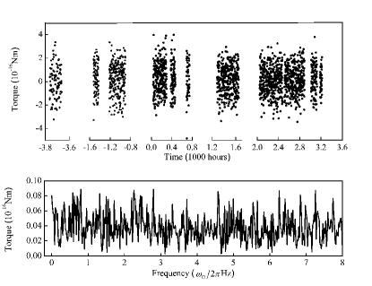
Figure 1: HUST-2015 data at $8f_{0}$ and Fourier transform.

For the HUST-2015 experiment, extraction of the LV signal from the data proceeds as described in Ref. hust-iu16 . The data rate is much faster than the attractor modulation frequency, so data are partitioned into bins corresponding to the modulation period $\Delta T=3846.12$ s. The LV torque signals $\tau_{{\rm LV},n}(T_{\oplus})$ with $n=8$ and 16 are extracted by fitting the measured torque $\tau^{z}(T_{\oplus})$ in each bin to

$${\tau^{z}}(T_{\oplus})=\sum\limits_{n=8,16}{{\tau_{{\rm LV},n}}(T_{\oplus})}\cos(2\pi n{f_{0}}T_{\oplus}+{\varphi_{n}}),$$ (10)

where ${\varphi_{n}}$ is set by operation of the experiment. The values of $\tau_{{\rm LV},n}(T_{\oplus})$ are taken to be approximately constant in each bin, since ${\omega_{\oplus}}\Delta T\ll 1$ and any sidereal variation within each bin is negligible. Data for the torque ${\tau_{{\rm LV},8}}$ are plotted in the upper panel of Fig. 1 as a function of time. Each point shows the mean measurement in the modulation period without errors, which are dominated by statistical fluctuations. The Fourier spectrum for these data is displayed in the lower panel of Fig. 1. The corresponding plots for the torque $\tau_{LV,16}$ appear in Fig. 1 of Ref. hust-iu16 .

Table 3: Fourier amplitudes ($2\sigma$, units $10^{-16}$ Nm for HUST and $10^{-16}$ N for IU).

Mode	HUST-8$f_{0}$	HUST-16$f_{0}$	IU-2012	IU-2002
${C_{0}}$	$0.08\pm 0.10$	$-0.20\pm 2.40$	$0\pm 136$	$2\pm 411$
${C_{2}}$	$0.00\pm 0.08$	$-0.01\pm 0.08$	$47\pm 166$	$-53\pm 556$
${S_{2}}$	$-0.06\pm 0.08$	$-0.08\pm 0.08$	$-192\pm 187$	$-51\pm 176$
${C_{4}}$	$0.00\pm 0.08$	$0.04\pm 0.08$	$-42\pm 156$	$25\pm 448$
${S_{4}}$	$0.01\pm 0.08$	$-0.03\pm 0.08$	$-58\pm 192$	$83\pm 237$
${C_{6}}$	$0.04\pm 0.08$	$-0.04\pm 0.08$	$-41\pm 179$	$61\pm 306$
${S_{6}}$	$0.00\pm 0.08$	$0.02\pm 0.08$	$91\pm 146$	$52\pm 241$
${C_{1}}$	$-0.03\pm 0.08$	$0.00\pm 0.08$	$-108\pm 193$	$30\pm 130$
${S_{1}}$	$0.03\pm 0.08$	$0.00\pm 0.08$	$3\pm 161$	$-192\pm 449$
${C_{3}}$	$0.00\pm 0.08$	$0.01\pm 0.08$	$-173\pm 145$	$215\pm 180$
${S_{3}}$	$0.03\pm 0.08$	$-0.06\pm 0.08$	$223\pm 207$	$-56\pm 390$
${C_{5}}$	$0.02\pm 0.08$	$-0.03\pm 0.08$	$142\pm 181$	$-98\pm 201$
${S_{5}}$	$-0.08\pm 0.08$	$0.05\pm 0.08$	$132\pm 165$	$-190\pm 290$

Table 4: Independent coefficient values (2$\sigma$, units 10^-13 m⁴) obtained by combining HUST and IU data.

	Coefficient	Measurement
	$k^{\rm N(8)}_{{4}{0}}{}$	$-6.4\pm 50.9$
	Re $k^{\rm N(8)}_{{4}{1}}{}$	$1.7\pm 5.5$
	Im $k^{\rm N(8)}_{{4}{1}}{}$	$0.9\pm 5.8$
	Re $k^{\rm N(8)}_{{4}{2}}{}$	$0.0\pm 3.9$
	Im $k^{\rm N(8)}_{{4}{2}}{}$	$0.9\pm 4.0$
	Re $k^{\rm N(8)}_{{4}{3}}{}$	$4.3\pm 7.3$
	Im $k^{\rm N(8)}_{{4}{3}}{}$	$2.4\pm 7.3$
	Re $k^{\rm N(8)}_{{4}{4}}{}$	$-2.8\pm 14.5$
	Im $k^{\rm N(8)}_{{4}{4}}{}$	$-2.9\pm 14.4$
	$k^{\rm N(8)}_{{6}{0}}{}$	$5.1\pm 100.9$
	Re $k^{\rm N(8)}_{{6}{1}}{}$	$-2.4\pm 5.9$
	Im $k^{\rm N(8)}_{{6}{1}}{}$	$-1.2\pm 6.4$
	Re $k^{\rm N(8)}_{{6}{2}}{}$	$1.9\pm 5.5$
	Im $k^{\rm N(8)}_{{6}{2}}{}$	$1.7\pm 6.2$
	Re $k^{\rm N(8)}_{{6}{3}}{}$	$4.7\pm 6.8$
	Im $k^{\rm N(8)}_{{6}{3}}{}$	$0.6\pm 7.9$
	Re $k^{\rm N(8)}_{{6}{4}}{}$	$-0.9\pm 6.8$
	Im $k^{\rm N(8)}_{{6}{4}}{}$	$-0.9\pm 6.7$
	Re $k^{\rm N(8)}_{{6}{5}}{}$	$1.2\pm 7.8$
	Im $k^{\rm N(8)}_{{6}{5}}{}$	$3.7\pm 7.1$
	Re $k^{\rm N(8)}_{{6}{6}}{}$	$5.7\pm 14.4$
	Im $k^{\rm N(8)}_{{6}{6}}{}$	$0.9\pm 14.2$

The Fourier amplitudes $C_{m},S_{m}$ are obtained by a subsequent fit of the $\tau_{{\rm LV},n}(T)$ data to Eq. (8), including a small correction for averaging over $\Delta T$ hust-iu16 . The results are shown in the second and third columns of Table 3. A residual Newton torque is subtracted from the time-independent amplitude $C_{0}$. The error on this amplitude is dominated by the uncertainties on the calculated Newton torque hust15-2 , which in turn arise primarily from uncertainties in the dimensions and positions of the test masses. The Newton torque and its error are considerably larger for the $16f_{0}$ component, which is less well nulled by the compensation scheme. The sidereal-harmonic amplitudes in Table 3 are dominated by the statistical uncertainty, which is at the same level for each harmonic.

For the the IU-2002 and IU-2012 experiments, the acquired force data are described in detail in Ref. lk15 . The corresponding Fourier amplitudes up to the sixth harmonic of the sidereal frequency $\omega_{\oplus}$ are listed in Table 3. Uncertainties are dominated by the statistical errors in the data. Errors also include contributions from the calibration jcl02 ; lk15 and from corrections due to discontinuities in the time-series data lk15 , the latter of which include here contributions from the $5\omega_{\oplus}$ and $6\omega_{\oplus}$ terms and hence display slight difference relative to the amplitudes reported in Ref. hust-iu16 . Note that a few modes at $2\omega_{\oplus}$ and $3\omega_{\oplus}$ seem to reveal potential resolved signals, but these subsequently become swamped by geometrical uncertainties of the transfer coefficients during the analysis and hence yield final measurements of $k_{jm}^{{\rm N(8)}}$ consistent with zero.

With the results in Table 3 in hand, the joint analysis proceeds as described in Refs. lk15 and hust-iu16 . A global probability distribution $P(\bm{\tilde{f}}|\bm{k})$ is formed using the 52 Fourier amplitudes $\tilde{f}_{i}$ in Table 3 and their errors. Each measured amplitude is assigned a gaussian distribution $p_{i}$ that is a function of the 22 independent $k_{jm}^{{\rm N(8)}}$ and has mean $\mu_{i}$ and standard deviation $\sigma_{i}$. The product of the individual $p_{i}$ defines the global distribution,

$$P(\bm{\tilde{f}}|\bm{k})=P_{0}\exp\left[-\sum_{i=1}^{52}\frac{(\tilde{f_{i}}-\mu_{i})^{2}}{2\sigma^{2}_{i}}\right],$$ (11)

where $P_{0}$ is an arbitrary normalization. The predicted signal $\mu_{i}$ for the $i$th amplitude is given by the appropriate Fourier component for the HUST or IU experiments, with the function $\alpha_{j}$ replaced by the associated integrated transfer coefficient $\Lambda_{j}$ in Table 2. The variance $\sigma_{i}^{2}$ incorporates all statistical and calibration errors. Following standard procedure pdg to account for the metrology errors on the $\mu_{i}$, the global distribution is replaced with the expression

$$P^{\prime}(\bm{\tilde{f}}|\bm{k})=\int P(\bm{\tilde{f}}|\bm{k},\bm{x})\pi(\bm{x})d\bm{x},$$ (12)

where $\bm{x}$ represents the set of geometry variables and $\pi(\bm{x})$ is their prior probability density function. For simplicity, for each geometry parameter $x$, $\pi(x)$ is taken to be a uniform distribution centered at the measured $x$ with a width of twice the error $\Delta x$, so that the integral (12) reduces to an average over $\bm{x}$. Independent measurements of each component $k_{jm}^{{\rm N(8)}}$ are then obtained by integrating $P^{\prime}(\bm{\tilde{f}}|\bm{k})$ over all other components. The result is a distribution for the chosen component with a single mean and standard deviation, which constitute the estimated component measurement and its error.

Table 4 displays the final results obtained from this joint HUST-IU analysis for the 22 independent coefficients $k_{jm}^{{\rm N(8)}}$ for LV in the Sun-centered frame. The results are consistent with no LV force varying according to the inverse sixth power, at the level of ${10^{-12}}$ m⁴. These measurements are the first of their kind, and they set a benchmark excluding short-range LV gravitational forces down to a distance scale of below a millimeter. They thereby enhance the scope of recent constraints on LV operators in pure gravity with $d=4$ bk06 ; 2007Battat ; 2007MullerInterf ; 2009Chung ; jcl10 ; 2010Panjwani ; 2010Altschul ; 2011Hohensee ; 2012Iorio ; 2013Bailey ; 2014Shao ; kt15 ; he15 ; bo16 ; yu16 ; pl16 ; bo17 ; 2016Flowers ; 2017Abbott ; 2017Shao $d=5$ km16 ; 2018Bailey , $d=6$ kt15 ; lk15 ; hust15 ; hust-iu16 ; km17 ; yu16 ; km16 $d=7$ km16 , $d=8$ kt15 , and $d=10$ jt16 .

This work was supported in part by the National Natural Science Foundation of China under grants No. 91636221, No. 11722542, No. 91736312, and No. 11805074, by the United States National Science Foundation under grant No. PHY-1707986, by the United States Department of Energy under grant No. DE-SC0010120, and by the Indiana University Center for Spacetime Symmetries.

References

- (1) V.A. Kostelecký and S. Samuel, Phys. Rev. D 39, 683 (1989); V.A. Kostelecký and R. Potting, Nucl. Phys. B 359, 545 (1991); Phys. Rev. D 51, 3923 (1995).
- (2) V.A. Kostelecký, Phys. Rev. D 69, 105009 (2004).
- (3) V.A. Kostelecký and N. Russell, Data Tables for Lorentz and CPT Violation, 2018 edition, arXiv:0801.0287v11.
- (4) For reviews see, A. Hees, Q.G. Bailey, A. Bourgoin, H. Pihan-Le Bars, C. Guerlin, and C. Le Poncin-Lafitte, Universe 2, 30 (2016); J.D. Tasson, Rept. Prog. Phys. 77, 062901 (2014); C.M. Will, Liv. Rev. Rel. 17, 4 (2014); R. Bluhm, Lect. Notes Phys. 702, 191 (2006).
- (5) For reviews see, for example, J. Murata and S. Tanaka, Class. Quant. Grav. 32 033001 (2015); J. Jaeckel and A. Ringwald, Ann. Rev. Nucl. Part. Sci. 60, 405 (2010); E.G. Adelberger, J.H. Gundlach, B.R. Heckel, S. Hoedl, and S. Schlamminger, Prog. Part. Nucl. Phys. 62, 102 (2009); E. Fischbach and C. Talmadge, The Search for Non-Newtonian Gravity, Springer-Verlag, 1999.
- (6) J.C. Long and V.A. Kostelecký, Phys. Rev. D 91, 092003 (2015).
- (7) C.-G. Shao, Y.-J. Tan, W.-H. Tan, S.-Q. Yang, J. Luo, and M.E. Tobar, Phys. Rev. D 91, 102007 (2015).
- (8) C.-G. Shao, Y.-J. Tan, W.-H. Tan, S.-Q. Yang, J. Luo, M.E. Tobar, Q.G. Bailey, J.C. Long, E. Weisman, R. Xu, and V.A. Kostelecký, Phys. Rev. Lett. 117, 071102 (2016).
- (9) Q.G. Bailey and V.A. Kostelecký, Phys. Rev. D 74, 045001 (2006).
- (10) Q.G. Bailey, V.A. Kostelecký, and R. Xu, Phys. Rev. D 91, 022006 (2015).
- (11) V.A. Kostelecký and M. Mewes, Phys. Lett. B 766, 137 (2017).
- (12) V.A. Kostelecký and M. Mewes, Phys. Lett. B 779, 136 (2018).
- (13) V.A. Kostelecký and J.D. Tasson, Phys. Rev. Lett. 102, 010402 (2009).
- (14) D. Colladay and V.A. Kostelecký, Phys. Rev. D 55, 6760 (1997); Phys. Rev. D 58, 116002 (1998).
- (15) R. Bluhm, V.A. Kostelecký, C.D. Lane, and N. Russell, Phys. Rev. D 68, 125008 (2003); Phys. Rev. Lett. 88, 090801 (2002); V.A. Kostelecký and M. Mewes, Phys. Rev. D 66, 056005 (2002).
- (16) V.A. Kostelecký, Phys. Rev. Lett. 80, 1818 (1998).
- (17) V.A. Kostelecký, A.C. Melissinos, and M. Mewes, Phys. Lett. B 761, 1 (2016); Y. Ding and V.A. Kostelecký, Phys. Rev. D 94, 056008 (2016).
- (18) E.P. Wigner, Group Theory, Academic, New York, 1959.
- (19) W.-H. Tan, S.-Q. Yang, C.-G. Shao, J. Li, A.-B. Du, B.-F. Zhan, Q.-L. Wang, P.-S. Luo, L.-C. Tu, and J. Luo, Phys. Rev. Lett. 116, 131101 (2016).
- (20) S.-Q. Yang, B.-F. Zhan, Q.-L. Wang, C.-G. Shao, L.-C. Tu, W.-H. Tan, and J. Luo, Phys. Rev. Lett. 108, 081101 (2012).
- (21) C.-G. Shao, Y.-F. Chen, Y.-J. Tan, W.-H. Tan, J. Luo, S.-Q. Yang, and M.E. Tobar, Phys. Rev. D 94, 104061 (2016).
- (22) J.C. Long, in V.A. Kostelecký, ed., CPT and Lorentz Symmetry VII, World Scientific, Singapore 2016.
- (23) E. Poisson and C.M. Will, Gravity: Newtonian, Post-Newtonian, Relativistic, Cambridge University Press, Cambridge, 2014.
- (24) V.A. Kostelecký and M. Mewes, Phys. Rev. D 80, 015020 (2009).
- (25) J.C. Long, H.W. Chan, A.B. Churnside, E.A. Gulbis, M.C.M. Varney, and J.C. Price, arXiv:hep-ph/0210004.
- (26) J.C. Long, H.W. Chan, A.B. Churnside, E.A. Gulbis, M.C.M. Varney, and J.C. Price, Nature 421, 922 (2003).
- (27) H. Yan, E.A. Housworth, H.O. Meyer, G. Visser, E. Weisman, and J.C. Long, Class. Quant. Grav. 31, 205007 (2014).
- (28) M. Tanabashi et al.. (Particle Data Group), Phys. Rev. D 98, 030001 (2018).
- (29) J.B.R. Battat, J.F. Chandler, and C.W. Stubbs, Phys. Rev. Lett. 99, 241103 (2007).
- (30) H. Müller, S.-w. Chiow, S. Herrmann, S. Chu, and K.-Y. Chung, Phys. Rev. Lett. 100, 031101 (2008).
- (31) K.-Y. Chung, S.-w. Chiow, S. Herrmann, S. Chu, and H. Müller, Phys. Rev. D 80, 016002 (2009).
- (32) D. Bennett, V. Skavysh, and J. Long, in V.A. Kostelecký, ed., CPT and Lorentz Symmetry V, World Scientific, Singapore 2011.
- (33) H. Panjwani, L. Carbone, and C.C. Speake, in V.A. Kostelecký, ed., CPT and Lorentz Symmetry V, World Scientific, Singapore 2011.
- (34) B. Altschul, Phys. Rev. D 82, 016002 (2010).
- (35) M.A. Hohensee, S. Chu, and H. Müller, Phys. Rev. Lett. 106, 151102 (2011).
- (36) L. Iorio, Class. Quant. Grav. 29, 175007 (2012).
- (37) Q.G. Bailey, R.D. Everett, and J.M. Overduin, Phys. Rev. D 88, 102001 (2013).
- (38) L. Shao, Phys. Rev. Lett. 112, 111103 (2014); Phys. Rev. D 90, 122009 (2014).
- (39) V.A. Kostelecký and J.D. Tasson, Phys. Lett. B 749, 551 (2015).
- (40) A. Hees, Q.G. Bailey, C. Le Poncin-Lafitte, A. Bourgoin, A. Rivoldini, B. Lamine, F. Meynadier, C. Guerlin, and P. Wolf, Phys. Rev. D 92, 064049 (2015).
- (41) A. Bourgoin, A. Hees, S. Bouquillon, C. Le Poncin-Lafitte, G. Francou, and M.-C. Angonin, Phys. Rev. Lett. 117, 241301 (2016).
- (42) N. Yunes, K. Yagi, and F. Pretorius, Phys. Rev. D 94, 084002 (2016).
- (43) C. Le Poncin-Lafitte, A. Hees, and S. Lambert, Phys. Rev. D 94, 125030 (2016).
- (44) N. Flowers, C. Goodge, and J.D. Tasson, Phys. Rev. Lett. 119, 201101 (2017).
- (45) A. Bourgoin, C. Le Poncin-Lafitte, A. Hees, S. Bouquillon, G. Francou, and M.-C. Angonin, Phys. Rev. Lett. 119, 201102 (2017).
- (46) B.P. Abbott et al., Astrophys. J. 848, L13 (2017).
- (47) C.-G. Shao et al., Phys. Rev. D 97, 024019 (2018).
- (48) V.A. Kostelecký and M. Mewes, Phys. Lett. B 757, 510 (2016).
- (49) L. Shao and Q.G. Bailey, Phys. Rev. D 98, 084049 (2018).
- (50) J.D. Tasson, Symmetry 8, 111 (2016).