Influence of technological progress and renewability on the sustainability of ecosystem engineers populations

Abstract

Overpopulation and environmental degradation due to inadequate resource-use are outcomes of human’s ecosystem engineering that has profoundly modified the world’s landscape. Despite the age-old concern that unchecked population and economic growth may be unsustainable, the prospect of societal collapse remains contentious today. Contrasting with the usual approach to modeling human-nature interactions, which are based on the Lotka-Volterra predator-prey model with humans as the predators and nature as the prey, here we address this issue using a discrete-time population dynamics model of ecosystem engineers. The growth of the population of engineers is modeled by the Beverton-Holt equation with a density-dependent carrying capacity that is proportional to the number of usable habitats. These habitats (e.g., farms) are the products of the work of the individuals on the virgin habitats (e.g., native forests), hence the denomination engineers of ecosystems to those agents. The human-made habitats decay into degraded habitats, which eventually regenerate into virgin habitats. For slow regeneration resources, we find that the dynamics is dominated by cycles of prosperity and collapse, in which the population reaches vanishing small densities. However, increase of the efficiency of the engineers to explore the resources eliminates the dangerous cyclical patterns of feast and famine and leads to a stable equilibrium that balances population growth and resource availability. This finding supports the viewpoint of growth optimists that technological progress may avoid collapse.

I Introduction

The gloomy consequences of rapid population growth and environmental degradation have been a major public concern, probably first expressed explicitly in the work of Thomas Malthus Malthus_98 , who believed that informed public policies could mitigate or even avoid altogether the happening of those circumstances. Following this line, in the 1970s the Club of Rome commissioned a major enterprise aiming at modeling the interactions between the earth and human systems using massive computer simulations capable of producing detailed near-future scenarios Meadows_72 ; Meadows_04 . Although efforts in that direction are still ongoing Randers_12 , this approach is somewhat abstruse as the complexity of the simulated models rivals that of the real-world, thus making it difficult to untangle the effects of the model parameters. An alternative approach to address such concerns, which we adopt here, is the study of minimal models that link the population dynamics and the resource dynamics. Works in this line typically build on Lotka-Volterra predator-prey models Murray_03 , where man is seen as the predator and the resource base as the prey Brander_98 ; Motesharrei_14 .

Yet the predator-prey approach to human-nature dynamics misses the important fact that humans do not primarily prey on nature but modify it. In fact, humans are the ultimate ecosystem engineers, who have shaped the world into a more hospitable place for themselves, most often with unlooked-for long term effects Smith_07 . One such effect is the collapse of human societies likely caused by habitat destruction and overpopulation Tainter_90 ; Diamond_05 , hence the public concern on this matter. Accordingly, here we argue that the baseline population dynamics model that is more suitable to address human-nature interactions is the ecosystem engineers model Jones_94 ; Gurney_96 , rather than the predator-prey model. The feature of the population dynamics of ecosystem engineers that makes this approach well suited to model those interactions is that the growth of the population is determined by the availability of usable habitats, which in turn are created by the engineers through the modification, and consequent destruction, of virgin habitats. From a mathematical perspective, this feedback results in a density-dependent carrying capacity that produces a very rich dynamic behavior both in the continuous-time Gurney_96 and the discrete-time formulations Franco_17 .

More pointedly, the Gurney and Lawton model for the population dynamics of ecosystem engineers describes the time evolution of the density of engineers and of the habitats, which can exist in three different forms: virgin, usable and degraded. The transition of a habitat from the virgin form to the usable form occurs due to the work of the engineers. The usable habitats then degrade and eventually recover to become virgin habitats again. Virgin and degraded habitats are unsuitable for the growth of the population. To expedite the numerical analysis, here we use a discrete-time approach where the logistic growth equation of the original model is replaced by the Beverton-Holt equation BH_57 . The weak nonlinearity of this equation prevents the large fluctuations on the population size produced by the Ricker equation Ricker_54 , which may result in a spurious chaotic dynamics Franco_17 .

We find that the survival of the population depends on two independent factors, viz., the competence of the engineers to transform natural resource base (e.g., native forests) into useful goods (e.g., farms) and the population growth rate per generation. Survival is guaranteed provided that the product of these two factors is greater than the decay rate per generation of the usable habitats. However, survival is not without adversities in the case the regeneration rate per generation of the degraded habitats is too slow. In this case, the dynamics exhibits cycles of prosperity and collapse, in which the population reaches vanishing small densities. Extinction does not occur because the fixed-point associated to it is unstable. The regime of cycles is favored by large population growth rates.

Most interestingly, we find that increase of the efficiency of the engineers to explore the resource base, thus modeling a high-tech society scenario where a few individuals can extract and produce the goods needed for survival, eliminates the dangerous cyclical patterns of feast and famine and leads to a smooth adjustment between population and resources. This finding supports the viewpoint of growth optimists that technological progress may avoid collapse.

In the case the resources are non-renewable, the long-term outcome is a doomsday scenario in which the ecosystem is reduced to degraded habitats only. Since the population is not immediately affected by the disappearance of the virgin habitats, we can interpret the usable habitats as a kind of wealth, i.e., surpluses that humans accumulate and that may extend their survival well beyond the point where the natural resources are exhausted. This observation offers a connection between ecosystem engineers models and economic models of human-nature interactions Motesharrei_14 .

The rest of the paper is organized as follows. In Section II, we introduce the discrete time version of Gurney and Lawton model of ecosystem engineers and derive the recursion equations for the density of engineers as well as for the fractions of the three forms of habitats. In that section we also derive and begin the analysis of the local stability of the fixed point solutions of those equations. Section III presents the results of the numerical study of the eigenvalues of the Jacobian matrices that determine the local stability of the fixed points as well as the results of the numerical iteration of the recursion equations. Finally, Section IV is reserved for our concluding remarks.

II Discrete-time population dynamics

The population dynamics of ecosystem engineering was modeled originally by Gurney and Lawton in the 1990s using a continuous-time model Gurney_96 , while discrete-time versions were considered only much more recently Franco_17 ; Fontanari_18 . We recall that the main advantage of discrete-time formulations is that they can easily be extended to incorporate a spatial dependence of the dynamic variables Kaneko_92 , as well as of the model parameters, as neatly demonstrated in the classic studies of the spatial dynamics of host-parasitoid systems Hassell_91 ; Comins_92 (see Rodrigues_11 ; Mistro_12 for more recent contributions). However, discrete-time nonlinear systems usually exhibit chaotic behavior, which is somewhat problematic from a biological perspective Berryman_89 and are not observed in their continuous-time counterparts Sprott_03 . Here we show that this drawback can be circumvented by a suitable choice of the equation that determines the growth of the population. In particular, whereas in previous studies the logistic equation of the continuous-time Gurney and Lawton model was replaced by the highly nonlinear Ricker equation Ricker_54 , here we use the growth equation of Beverton and Holt BH_57 , whose much weaker nonlinearity greatly limits the between-generations fluctuations and produces a stauncher representation of the continuous-time model.

We assume that the population of engineers at generation $t$ is composed of $E_{t}$ individuals and that the carrying capacity of the environment depends on the number of units of usable habitats available at generation $t$, which we denote by $H_{t}$. Thus, using the Beverton-Holt equation we write the expected number of engineers at generation $t+1$ as

$$E_{t+1}=rE_{t}/\left(1+E_{t}/H_{t}\right)$$ (1)

where $r>1$ is the intrinsic growth rate of the population of engineers and the time-dependent carrying capacity is $\left(r-1\right)H_{t}$. This model describes a system of ecosystem engineers due to the assumption that the usable habitats are produced by engineers working on virgin habitats Gurney_96 . More pointedly, assuming that there are $V_{t}$ units of virgin habitats at generation $t$, a fraction $C\left(E_{t}\right)V_{t}$ of them will be transformed in usable habitats by the engineers at the next generation $t+1$. Here $C\left(E_{t}\right)$ is any function that satisfies $0\leq C\left(E_{t}\right)\leq 1$ for all $E_{t}$ and $C\left(0\right)=0$. In other words, if there are no engineers at generation $t$, then virgin habitats cannot be transformed in usable ones. Hence $C\left(E_{t}\right)$ measures the efficiency of the engineer population to build usable habitats from the raw materials provided by the virgin habitats.

Usable habitats decay into degraded habitats that are useless to the engineers, in the sense that they are inhabitable and lack the raw materials needed to build usable habitats. Denoting by $\delta\in\left[0,1\right]$ the probability that a unit of usable habitat decays and becomes a unit of degraded habitat in one generation, we write the expected number of units of usable habitats at generation $t+1$ as

$$H_{t+1}=\left(1-\delta\right)H_{t}+C\left(E_{t}\right)V_{t}.$$ (2)

In this paper we assume that the decay probability $\delta$ is a density independent parameter. We recall that in the Gurney and Lawton model the resources are represented by the virgin habitats, whose probability of change into usable habitats is density dependent, i.e. $C=C\left(E_{t}\right)$. For example, in an island scenario, the virgin habitats can be thought of as the native forests whereas the usable habitats are the lands cleared for crops, whose degradation, due mainly to erosion and soil depletion of nutrients, is more suitably modeled by a constant decay probability $\delta$, rather than by a density-dependent one. (i.e., $\delta=\delta\left(E_{t}\right)$). However, in an economic context where the habitats represent, for instance, oil wells, the decay probability should be modeled by a density-dependent parameter, of course.

To take into account the possibility that the degraded habitats will eventually recover and become virgin habitats again, we introduce the parameter $\rho\in\left[0,1\right]$ that gives the probability that one unit of degraded habitat becomes one unit of virgin habitat in one generation. Thus, denoting the units of degraded habitats at generation $t$ by $D_{t}$ we write

$$D_{t+1}=\left(1-\rho\right)D_{t}+\delta H_{t}.$$ (3)

Thus $\rho$ is the regeneration rate per generation that measures the renewability of the resource base. Finally, recalling that virgin habitats are destroyed by the action of the engineers and created by the restoration of the degraded habitats, we write the recursion equation for the expected number of units of virgin habitats as

$$V_{t+1}=\left[1-C\left(E_{t}\right)\right]V_{t}+\rho D_{t},$$ (4)

which completes the description of the feedback interactions between habitats and engineers.

Since habitats can only be transformed from one form to another, the total number of units of habitats $V_{t+1}+H_{t+1}+D_{t+1}=V_{t}+H_{t}+D_{t}=T$ is conserved. This fact allows us to introduce the habitat fractions $v_{t}\equiv V_{t}/T$, $h_{t}\equiv H_{t}/T$ and $d_{t}\equiv D_{t}/T$ that satisfy $v_{t}+h_{t}+d_{t}=1$ for all $t$. Accordingly, we define also the density of engineers $e_{t}=E_{t}/T$ that, differently from the habitat fractions, may take on values greater than 1. In terms of these intensive quantities, the above recursion equations are rewritten as

$$e_{t+1} = re_{t}/\left(1+e_{t}/h_{t}\right)$$ (5)

$$h_{t+1} = \left(1-\delta\right)h_{t}+c\left(e_{t}\right)v_{t}$$ (6)

$$v_{t+1} = \rho\left(1-v_{t}-h_{t}\right)+\left[1-c\left(e_{t}\right)\right]v_{t},$$ (7)

where we have used $d_{t}=1-v_{t}-h_{t}$ and $c\left(e_{t}\right)\equiv C\left(Te_{t}\right)$.

To complete the model we must specify the density-dependent probability $c\left(e_{t}\right)$, which measures the engineers’ efficiency to transform the virgin habitats into usable ones. The function $c\left(e_{t}\right)$ incorporates the cooperation strategies used to build structures (e.g., beaver dams, termite mounds and anthills) to respond to external and internal threats to the population survival Francisco_16 ; Reia_17 . For humans, this function incorporates the beneficial effects (from their perspective) of the technological advancements that enable a more efficient harvesting of natural resources Basalla_89 . Here we consider the continuous function

$$c\left(e_{t}\right)=\left\{\begin{array}[]{c l}\alpha e_{t}+\left(1-\alpha\right)e_{t}^{2}&\mbox{if $e_{t}<1$}.\\ 1&\mbox{if $e_{t}\geq 1$}.\end{array}\right.$$ (8)

where $\alpha\in\left[0,1\right]$ is the efficiency parameter that measures the competence of the engineers in transforming natural resources into useful goods. The range of variation of $\alpha$ guarantees that $c\left(e_{t}\right)\leq 1$ regardless of the value of $e_{t}$. For $\alpha\ll 1$ we have a scenario where the efficient exploration of the virgin habitats requires a high density of engineers. In this low-tech scenario, we expect to observe an Allee effect, in which the population quickly goes extinct below a critical density Courchamp_08 . We note that when $e_{t}>1$ all the available virgin habitats are transformed into usable ones in just a single generation. This arbitrary threshold value does not produce any significant effect on our results since we find that $e_{t}<1$ at all times in the parameter regions of interest, i.e., in the regions close to the transitions between the fixed point attractors and the limit cycles.

II.1 Fixed-point solutions

In this section we study the fixed-point solutions of the system of recursion equations (5)-(7) that are obtained by setting $e_{t+1}=e_{t}=e^{*}$, $h_{t+1}=h_{t}=h^{*}$ and $v_{t+1}=v_{t}=v^{*}$. Next we consider separately the two cases, $e^{*}=0$ (zero-engineers fixed point) and $e^{*}>0$ (finite-engineers fixed point). The local stability of the fixed point solutions are determined by the eigenvalues of the Jacobian matrix of the system of recursion equations (5), (6), (7),

$$J_{e_{t}}=\begin{bmatrix}r/\left(1+x_{t}\right)^{2}&~{}~{}~{}~{}r\left[x_{t}/\left(1+x_{t}\right)\right]^{2}&~{}~{}~{}~{}0\\ v_{t}c^{\prime}\left(e_{t}\right)&~{}~{}~{}~{}1-\delta&~{}~{}~{}~{}c\left(e_{t}\right)\\ -v_{t}c^{\prime}\left(e_{t}\right)&~{}~{}~{}~{}-\rho&~{}~{}~{}~{}1-\rho-c\left(e_{t}\right)\end{bmatrix},$$ (9)

where $x_{t}=e_{t}/h_{t}$ and $c^{\prime}\left(e_{t}\right)=dc\left(e_{t}\right)/de_{t}$.

II.1.1 Zero-engineers fixed point

In the absence of the engineers (i.e., $e^{*}=0$) all usable habitats will degrade and then recover to virgin habitats (provided that $\rho>0$), so we have $h^{*}=0$ and $v^{*}=1$. To circumvent the indetermination of the ratio $e^{*}/h^{*}$, we write an equation for $x_{t}$ dividing eq. (5) by eq.  (6),

$$x_{t+1}=\frac{rx_{t}}{\left(1+x_{t}\right)\left[1-\delta+x_{t}v_{t}\hat{c}\left(e_{t}\right)\right]},$$ (10)

where $\hat{c}\left(e_{t}\right)=c\left(e_{t}\right)/e_{t}$. Thus the fixed point $x_{t+1}=x_{t}=x^{*}>0$ is given by the positive solution of the quadratic equation

$$\left(1+x^{*}\right)\left[1-\delta+\alpha x^{*}\right]=r,$$ (11)

where we have used $\hat{c}\left(0\right)=\lim_{e^{*}\to 0}c\left(e^{*}\right)/e^{*}=c^{\prime}\left(0\right)=\alpha$. The quadratic equation (11) has two real roots, one positive and the other negative, for all values of the model parameters. In particular, for $\delta=\alpha\left(r-1\right)$ the solution is $x^{*}=r-1$ and we can easily show that $x^{*}>r-1$ for $\delta>\alpha\left(r-1\right)$ and $x^{*}<r-1$ for $\delta<\alpha\left(r-1\right)$, a result that will proven helpful to verify the local stability of this fixed point.

In fact, the local stability of the zero-engineers fixed point is determined by requiring that the three eigenvalues of the Jacobian matrix

$$J_{e^{*}=0}=\begin{bmatrix}r/\left(1+x^{*}\right)^{2}&~{}~{}~{}~{}r\left[x^{*}/\left(1+x^{*}\right)\right]^{2}&~{}~{}~{}~{}0\\ \alpha&~{}~{}~{}~{}1-\delta&~{}~{}~{}~{}0\\ -\alpha&~{}~{}~{}~{}-\rho&~{}~{}~{}~{}1-\rho\end{bmatrix}$$ (12)

have norms less than 1. The eigenvalues of the Jacobian matrix (12) are $\lambda_{1}=r/\left(1+x^{*}\right)$, $\lambda_{2}=r/\left(1+x^{*}\right)^{2}-\alpha x^{*}$ and $\lambda_{3}=1-\rho$. The condition $\mid\lambda_{1}\mid<1$ is satisfied provided that $x^{*}>r-1$, which is guaranteed for $\delta>\alpha\left(r-1\right)$, whereas the condition $\mid\lambda_{3}\mid<1$ is always satisfied since $\rho<1$. The proof that the condition $\mid\lambda_{2}\mid<1$ is always satisfied whenever $\lambda_{1}<1$ is very simple. Since $\alpha>0$ and $x^{*}>0$ we can write $\lambda_{2}<r/\left(1+x^{*}\right)^{2}=\lambda_{1}/\left(1+x^{*}\right)<1/\left(1+x^{*}\right)<1$. Next we need to show that $\lambda_{2}>-1$. To do so we use eq. (11) to write $\alpha x^{*}=\lambda_{1}-1+\delta$ so that $\lambda_{2}=1-\delta-x^{*}\lambda_{1}/\left(1+x^{*}\right)>1-\delta-1>-\delta>-1$.

We note that this stability analysis describes the convergence (or divergence) of the system of recursion equations for $e_{t}$, $h_{t}$ and $v_{t}$, eqs. (5), (6) and (7), respectively, to the fixed point $e^{*}=h^{*}=0$ and $v^{*}=1$ and that equations (10) and (11) were used only to specify the ratio $\lim_{t\to\infty}e_{t}/h_{t}$ that is required to evaluate the Jacobian (9). We mention this because use of recursion equations for $e_{t}$, $x_{t}$ and $v_{t}$ instead, yields a different Jacobian for the zero-engineers fixed point, which exhibits the same eigenvalues $\lambda_{1}$ and $\lambda_{3}$ as the Jacobian (12), but a different eigenvalue $\lambda_{2}$. However, the local stability of the fixed point is again determined solely by the norm of the common eigenvalue $\lambda_{1}$ so this issue has no effect in our findings regarding the zero-engineers fixed point.

In sum, the condition for the stability of the zero-engineers fixed point is $\delta<\alpha\left(r-1\right)$, which, as expected, does not depend on the regeneration rate $\rho$ since there is no shortage of virgin habitats (i.e., $v_{t}\approx 1$) in the vicinity of this fixed point.

II.1.2 Finite-engineers fixed point

Since $e^{*}>0$ we have $h^{*}=e^{*}/\left(r-1\right)$ and $v^{*}=1-e^{*}\gamma/\left(r-1\right)$ with $e^{*}$ given by the solution of the equation

$$\delta e^{*}=c\left(e^{*}\right)\left[r-1-e^{*}\gamma\right],$$ (13)

where we have introduced the notation $\gamma=\left(1+\delta/\rho\right)$.

Let us assume that $e^{*}<1$ so we can use eq. (8) to rewrite eq. (13) as the quadratic equation

$$\left(1-\alpha\right)\gamma(e^{*})^{2}-e^{*}\left[\left(1-\alpha\right)\left(r-1\right)-\alpha\gamma\right]+\delta-\alpha\left(r-1\right)=0.$$ (14)

The local stability of the two solutions of this equation is determined by the the Jacobian matrix (9) that is rewritten as

$$J_{e^{*}<1}=\begin{bmatrix}1/r&~{}~{}~{}~{}\left(r-1\right)^{2}/r&~{}~{}~{}~{}0\\ v^{*}c^{\prime}\left(e^{*}\right)&~{}~{}~{}~{}1-\delta&~{}~{}~{}~{}c\left(e^{*}\right)\\ -v^{*}c^{\prime}\left(e^{*}\right)&~{}~{}~{}~{}-\rho&~{}~{}~{}~{}1-\rho-c\left(e^{*}\right)\end{bmatrix}.$$ (15)

The main difficulty of the analysis of the eigenvalues of this Jacobian matrix is that two eigenvalues are complex, leading to the enthralling dynamic behavior exhibited by the recursion equations (5), (6), (7) with the prescription (8). However, this problem can easily be solved numerically as follows. First we determine the critical points of the characteristic cubic polynomial, which allows us to obtain one real root of the characteristic equation with high numerical accuracy using the bisection method. (We recall that the critical points of a function are those values of the variable where the slope of the function is zero.) Then this root is factored out and the remaining roots of the characteristic equation are found by solving a quadratic equation. Actually, in the case of complex roots, we do no need to solve this quadratic equation since the local stability is determined by the norm of those roots that is given by the square root of the ratio between the constant and the quadratic coefficient. The fixed point solution is locally stable provided that the norms of all three roots of the characteristic polynomial are less than 1. We find that the smaller root of the fixed-point equation (14) is always locally unstable.

Now we consider the case $e^{*}>1$. Equation (13) yields

$$e^{*}=\frac{r-1}{1+\delta\left(1+1/\rho\right)}$$ (16)

that holds for $\delta<\left(r-2\right)/\left(1+1/\rho\right)$. In this case, the Jacobian matrix (9) becomes

$$J_{e^{*}>1}=\begin{bmatrix}1/r&~{}~{}~{}~{}\left(r-1\right)^{2}/r&~{}~{}~{}~{}0\\ 0&~{}~{}~{}~{}1-\delta&~{}~{}~{}~{}1\\ 0&~{}~{}~{}~{}-\rho&~{}~{}~{}~{}-\rho\end{bmatrix}.$$ (17)

Hence $\lambda_{1}=1/r<1$ is always a root of the characteristic polynomial and the other two roots are given by the quadratic equation $g\left(\lambda\right)=\lambda^{2}-\lambda\left(1-\rho-\delta\right)+\rho\delta=0$. In the case of complex roots, we have $\mid\lambda\mid^{2}=\rho\delta<1$. In the case of real roots, we use that $g(1)>0$ and $g(-1)>0$ and that the critical point of $g(\lambda)$ is between $-1$ and $1$ to guarantee that the absolute value of those roots are less than 1. Hence the fixed point (16) is always locally stable.

III Results

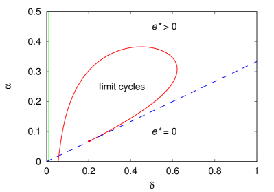
Figure 1: Regions in the space of the parameters $\left(\delta,\alpha\right)$ where the fixed points $e^{*}=0$ and $0<e^{*}<1$ are locally stable for $r=4$ and $\rho=0.005$. The dashed blue line $\alpha=\delta/3$ delimits the region of stability of the zero-engineers fixed point. There is a region of bistability for $\alpha<\delta/3$ and $\delta<0.055$. The limit cycles appear only in the regions where the fixed points are unstable. The fixed point $e^{*}>1$ exists and is stable only in the region to the left of the vertical green line at $\delta=2/201\approx 0.01$. The red bullet indicates the value of $\delta$ beyond which the transition over the dashed line is continuous.

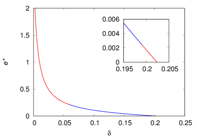
Figure 2: Fixed-point values of the density of engineers $e^{*}$ as function of the decay probability $\delta$ at the transition line $\alpha=\delta/\left(r-1\right)$ for $r=4$ and $\rho=0.005$. The fixed point is stable in the red segment of the curve and unstable in the blue segment. The inset shows that the finite-engineers fixed point becomes stable again close to the point where it vanishes, indicated by the red bullet in Fig. 1.

The local stability of the fixed points $e^{*}=0$ and $0<e^{*}<1$ is determined by the requirement that the norms of the eigenvalues of the Jacobian matrices (12) and (15), respectively, are less than 1. Accordingly, Fig.  1 shows the regions of stability of those fixed points. There is a large region in the space of parameters $\left(\delta,\alpha\right)$ where the fixed points are unstable and the solutions of the recursion equations exhibit periodic behavior. The drop-shaped region delimits the regions of stability of the finite-engineers fixed point.

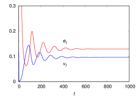
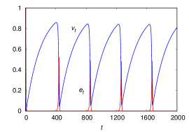
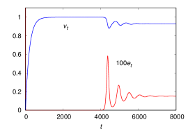
Figure 3: Density of engineers $e_{t}$ (red curves) and fraction of virgin habitats $v_{t}$ (blue curves) for $r=4$, $\rho=0.005$, $\alpha=0.25$ and $\delta=0.1$ (left panel), $\delta=0.4$ (middle panel) and $\delta=0.7$ (right panel). In the right panel, the density of engineers is magnified by a factor 100 in order to be visible in the scale of the figure.

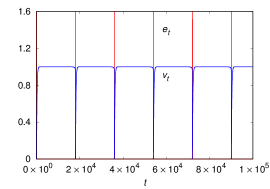
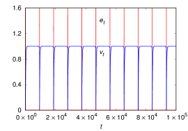
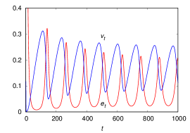
Figure 4: Density of engineers $e_{t}$ (red curves) and fraction of virgin habitats $v_{t}$ (blue curves) for $r=4$, $\rho=0.005$, $\delta=0.15$ and $\alpha=0.0505$ (left panel), $\alpha=0.051$ (middle panel) and $\alpha=0.24$ (right panel).

To better understand the results shown in Fig.  1, we first examine whether eq. (14) admits a physical solution with a vanishingly small density of engineers. In fact, for $e^{*}\ll 1$ we have

$$e^{*}\approx\frac{\alpha\left(r-1\right)-\delta}{\alpha\gamma-\left(1-\alpha\right)\left(r-1\right)},$$ (18)

so that the density of engineers vanishes continuously as the line $\alpha=\delta/\left(r-1\right)$ is approached from the region of large $\alpha$, provided the denominator in eq. (18) is positive. i.e., $\alpha\gamma-\left(1-\alpha\right)\left(r-1\right)>0$. In Fig. 1 we indicate with a red bullet the point $\delta=\delta_{c}\approx 0.202$ and $\alpha=\alpha_{c}\approx 0.067$ at which both the numerator and the denominator in eq. (18) vanish, meaning that $e^{*}=0$ is a double root of the quadratic equation (14). Thus, there is a continuous transition between the finite and the zero-engineers fixed point at $\alpha=\delta/\left(r-1\right)$ for $\delta>\delta_{c}$.

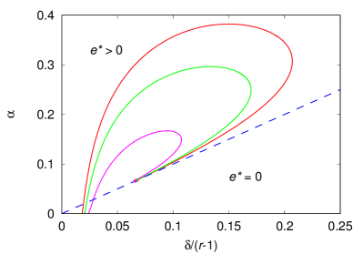
Figure 5: Regions in the space of the parameters $\left(\delta,\alpha\right)$ where the fixed points are locally stable for $\rho=0.005$ and $r=4$ (red curve), $r=3$ (green curve) and $r=2$ (magenta curve). The conventions for the labelling of the regions are the same as in Fig. 1, but we have omitted the regions where the fixed point $e^{*}>1$ appears. The zero-engineers fixed point is stable below the dashed blue line $\alpha=\delta/\left(r-1\right)$.

Next, we focus on the fixed-point solutions at the transition line $\alpha=\delta/\left(r-1\right)$. In this case, eq. (14) has the solution $e^{*}=0$ and

$$e^{*}=\frac{\left(1-\alpha\right)\left(r-1\right)-\alpha\gamma}{\left(1-\alpha\right)\gamma},$$ (19)

provided that $\alpha>\left(r-1\right)/\left(\left(r-1\right)-\gamma\right)$, which guarantees that $e^{*}<1$. Otherwise, we have $e^{*}=\left(r-1\right)/\left(\delta+\gamma\right)>1$ (see Section II.1.2). Figure 2 shows the finite-engineers fixed points at the transition, where the stable and unstable segments are flagged with different colors. The figure reveals that the fixed point $e^{*}>0$ is stable for small $\delta$, as expected, and that it is also stable close to the point $(\delta_{c},\alpha_{c})$. This indicates that this point does not belong to the drop-shaped curve shown in Fig. 1, which delimits the regions of stability of the finite-engineers fixed point. This facet will become much more evident when we consider larger values of the recovery probability $\rho$.

Another interesting feature of Fig.  1 is the appearance of a region of bistability of the two fixed points for small values of $\delta$ and $\alpha<\delta/3$. The dependence on the initial density of engineers, as well as on the initial habitats fractions, that characterizes the bistability regime results in an Allee effect where the environment cannot sustain a low density of engineers, as the change of the virgin habitats into usable ones can only be achieved by high-density populations.

Figure 3 illustrates the time dependence of the density of engineers $e_{t}$ and of the fraction of virgins habitats $v_{t}$ for three representative regions of Fig.  1, where the zero-engineers fixed point ($e^{*}=0$) is unstable, i.e, for $\delta<\alpha\left(r-1\right)$, so the results do not depend on the initial conditions. The time dependence of the fraction of usable habitats $h_{t}$ is similar to that of $e_{t}$. The recursion equations (5)-(7) were iterated using quadruple precision. The oscillatory convergence to the finite-engineers fixed point ($e^{*}>0$) is the effect of the complex eigenvalues of the Jacobian matrix (15). These oscillations may lead to extremely low values of the density engineers (e.g., $e_{t}$ on the order of $10^{-10}$), hence the need of a high precision numerical scheme to iterate the recursion equations. Since $e^{*}=0$ is unstable, the population eventually recovers from these near-extinction events as illustrated in the middle and right panels of Fig.  3.

The nature of the transition between the periodic solutions and the zero-engineers fixed point is clarified in Fig. 4 where we fix the decay rate per generation to $\delta=0.15$ and show $e_{t}$ and $v_{t}$ for different values of $\alpha$ in distinct panels. The left and middle panels, which show results for values of $\alpha$ very close to the stability boundary $\alpha=0.05$, reveal what happens: the period of the oscillations increases as that boundary is approached and diverges when the zero-engineers fixed point becomes stable, so that $e^{*}=0$ and $v^{*}=1$ for all times. The right panel in Fig. 4 reminds us that the periodic solutions are not necessarily associated to near-extinction events and that they can reproduce smooth oscillations with the usual phase shift of one-quarter of a cycle between engineers and virgin habitats, which characterizes the predator-prey models Turchin_03 .

Next we consider the effects of varying the parameters $r$ and $\rho$ that were kept fixed in the above analysis. Figure 5 shows the regions of stability of the fixed points for three values of the intrinsic growth rate $r$. To keep the size of the region where the zero-engineers fixed point is stable we use the scaled variable $\delta/\left(r-1\right)$ as the independent variable. The results indicate that increase of $r$ increases the size of the regions of limit cycles and decreases the size of the regions of bistability, so variation of $r$ produces quantitative effects only. This is in stark contrast with the effects of varying the regeneration rate per generation $\rho$ shown in Fig. 6. In fact, increase of $\rho$ decreases the size of the region of limit cycles, which eventually disappears altogether for large $\rho$, since there is no region left in the space of parameters where the fixed points $e^{*}>0$ and $e^{*}=0$ are simultaneously unstable. For instance, the curve for $\rho=0.3$ shown in the right panel of Fig. 6 is given by the condition that the discriminant of the quadratic equation (14) is zero, so for large $\rho$ the finite-engineers fixed point is locally stable wherever it is real. The piecewise curve for $\rho=0.1$ is given by the composition of the conditions that $e^{*}$ is real and that the norms of the eigenvalues of the Jacobian (15) are less than 1. In addition, increase of $\rho$ greatly increases the region of bistability as well as the region where $e^{*}>1$.

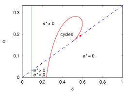
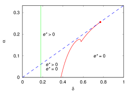
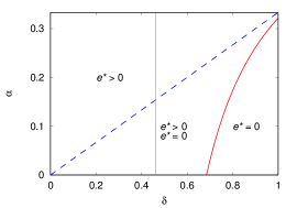
Figure 6: Regions in the space of the parameters $\left(\delta,\alpha\right)$ where the fixed point solutions are locally stable for $r=4$ and $\rho=0.05$ (left panel), $\rho=0.1$ (middle panel) and $\rho=0.3$ (right panel). The zero-engineers fixed point is stable below the dashed blue line $\alpha=\delta/3$. The fixed point $e^{*}>1$ exists and is stable only in the regions to the left of the vertical green lines. The bullets at the dashed line indicate the values of $\delta$ above which the transition between the finite and the zero-engineers fixed points is continuous.

To conclude, we consider now a simple but instructive scenario where the natural resources are not renewable, i.e., $\rho=0$. Figure 7 shows the time evolution of the population towards the doomsday fixed point $v^{*}=e^{*}=h^{*}=0$ and $d^{*}=1$ where only the degraded habitats are left. We have not considered this fixed point in Section II.1.1 because it exists and is stable solely for $\rho=0$ and $\delta>0$, regardless of the values the other model parameters. The interesting aspect this figure highlights is that the population survives for a long time after the irreversible disappearance of the virgin habitats, thus revealing that the usable habitats introduce a delay on the influence of the virgin habitats on the population that is absent in the usual predator-prey models. However, this delay appears in more sophisticated models of human-nature interactions in which humans accumulate surpluses (i.e., wealth) and use them when natural resources are scarce or unavailable Motesharrei_14 .

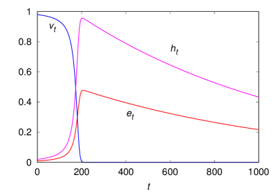
Figure 7: Density of engineers $e_{t}$ (red curves), fraction of virgin habitats $v_{t}$ (blue curves) and fraction of usable habitats $h_{t}$ (magenta curves) for $r=1.5$, $\rho=0$, $\delta=0.001$ and $\alpha=0.01$. The dynamics is attracted to the doomsday fixed point $v^{*}=e^{*}=h^{*}=0$ and $d^{*}=1$.

IV Discussion

The derivation of the discrete-time recursion equations (5)-(8) assumes non-overlapping generations, which is clearly not the case for human populations. Our justification to use this approach is purely pragmatic since it is much easier and much less error-prone to iterate those recursions than to solve numerically the differential equations of a continuous-time model, particularly in the region of reversible collapses where the density of engineers is very close to zero and the periods of the limit cycles are exceedingly long. However, as the solutions do not exhibit short-time fluctuations and are all smooth in the scale of a few generations we do not expect any significant differences between the discrete and the continuous time approaches. In addition, the discrete-time approach can easily be extended to describe space-dependent problems, resulting in coupled map lattices that can be thoroughly studied numerically. In particular, in this context a different type of population collapse can be observed when the expanding colonies of engineers reach the boundaries of their territories, thus ending the exploration of new virgin habitats and resulting in a sharp drop on the population density Fontanari_18 .

In agreement with the findings for the predator-prey type models Brander_98 ; Motesharrei_14 , we find that a key parameter to determine the long-term outcome of the population dynamics of ecosystem engineers is the regeneration rate per generation $\rho$, which determines the renewability of the resource base (see Fig. 6). Cycles of prosperity, collapse and revival occur in the case the degraded habitats have a slow regeneration rate. In the extreme case of non-renewable resources (i.e., $\rho=0$), the outcome of the dynamics is the irreversible collapse of the entire ecosystem (see Fig. 7). In the other extreme, when the degraded habitats rapidly recover into virgin habitats, the limit cycles disappear altogether and the outcome of the dynamics is determined by the basins of attraction of the finite and zero-engineers fixed points.

The local stability analysis of the zero-engineers fixed point yields a simple condition for the survival of the population, viz., the product of the parameter that measures the effective population growth rate (i.e., $r-1$) and the parameter that measures the efficiency of the transformation of virgin into usable habitats (i.e., $\alpha$) must be greater than the decay rate per generation of the usable habitats, i.e., $\alpha\left(r-1\right)>\delta$. Hence increase of the efficacy of the engineers to explore the virgin habitats or increase of their intrinsic effective growth rate will both guarantee the survival of the population, regardless of the regeneration rate $\rho>0$ of the degraded habitats. The characteristics of the steady-states for large $r$ and large $\alpha$, however, are completely distinct.

On the one hand, increase of $r$ favors limit cycles characterized by long periods of time when $e_{t}\ll 1$, which we refer to as reversible collapses. These collapses are reversible because they occur in regions of the model parameters where the zero-engineers fixed point is unstable. This scenario is expected since a large value of $r$ produces a large density of engineers, which, according to the prescription (8), can transform all virgin habitats in a single generation, thus producing the cyclical pattern of feast and famine illustrated in the left and middle panels of Fig. 4.

On the other hand, increase of $\alpha$ favors the finite-engineers fixed points and leads to a stable balance between population and resources. In our setup, a small $\alpha$ corresponds to a low-tech society where the exploration of the virgin habitats requires a high density of individuals. Interestingly, our model predicts that technology improvements that allow a small population to explore efficiently the available natural resources, a situation that is modeled by increasing $\alpha$ while keeping all the other parameters fixed, can eliminate the dangerous cycles of prosperity, collapse and revival.

This result is especially notable because it neatly expresses the argument put forward by the growth optimists, namely, that technological progress can reduce the impact of resource depletion and avoid environmental and economic collapse Atkisson_10 . Of course, this happens because our model does not account (among many other things) for the Jevons effect that occurs when technological progress increases the efficiency with which a resource is extracted, but the rate of consumption of that resource rises due to increasing demand Polimeni_15 . In our model, increasing demand amounts to considering the decay rate per generation dependent on the availability of usable habitats, i.e., $\delta=\delta\left(h_{t}\right)$, so that the more goods are available, the higher their consumption by the population. The possibility of supporting the growth optimists viewpoints as well as addressing quantitatively the Jevons effect, the analysis of which we postpone for a future contribution, highlights the potential of the ecosystem engineers approach to model both ecological and economic aspects of the human-nature dynamics.

- (1) T. R. Malthus, An essay on the theory of population, Oxford University Press, Oxford, 1798.
- (2) D. H. Meadows, D. L. Meadows, J. Randers and W. W. Behrens III, The Limits to Growth; A Report for the Club of Rome’s Project on the Predicament of Mankind, Universe Books, New York, 1972.
- (3) D. H. Meadows, J. Randers and D. L. Meadows Limits To Growth: The 30-Year Update, Chelsea Green Publishing, Vermont, 2004.
- (4) J. Randers, 2052: A Global Forecast for the Next Forty Years, Chelsea Green Publishing, Vermont, 2012.
- (5) J. D. Murray, Mathematical Biology: I. An Introduction, 3rd edition, Springer, New York, 2003.
- (6) J. A. Brander and M. S. Taylor, The Simple Economics of Easter Island: A Ricardo-Malthus Model of Renewable Resource Use, Am. Econ. Rev., 88 (1998), 119-138.
- (7) S. Motesharrei, J. Rivas and E. Kalnay, Human and nature dynamics (HANDY): Modeling inequality and use of resources in the collapse or sustainability of societies, Ecol. Econom., 101 (2014), 90–102.
- (8) B. D. Smith, The Ultimate Ecosystem Engineers, Science, 315 (2007), 1797–1798.
- (9) J. A. Tainter, The Collapse of Complex Societies, Cambridge University Press, Cambridge, UK, 1990.
- (10) J. Diamond, Collapse: How Societies Choose to Fail or Succeed, Penguin Books, New York, 2005.
- (11) C. G. Jones, J. H. Lawton and M. Shachak, Organisms as ecosystem engineers Oikos, 69 (1994), 373–386.
- (12) W. S. C. Gurney and J. H. Lawton, The population dynamics of ecosystem engineers, Oikos, 76 (1996), 273–283.
- (13) C. Franco and J. F. Fontanari, The spatial dynamics of ecosystem engineers, Math. Biosci., 292 (2017), 76–85.
- (14) R. J. H. Beverton and S. J. Holt, On the Dynamics of Exploited Fish Populations, Blackburn Press, Caldwell, NJ, 1993.
- (15) W. E. Ricker, Stock and Recruitment, J. Fish. Res. Bd. Canada, 11 (1954), 559–623.
- (16) J. F. Fontanari, The Collapse of Ecosystem Engineer Populations, Mathematics, 6 (2018), 9.
- (17) K. Kaneko, Overview of Coupled Map Lattices, Chaos, 2 (1992), 279–282.
- (18) M. P. Hassell, H. N. Comins and R. M. May, Spatial structure and chaos in insect population dynamics, Nature, 353 (1991), 255–258.
- (19) H. N. Comins, M. P. Hassell and R. M. May, The spatial dynamics of host-parasitoid systems, J. Anim. Ecol., 61 (1992) , 735–748.
- (20) L. A. D. Rodrigues, D. C. Mistro and S. Petrovskii, Pattern Formation, Long-Term Transients, and the Turing-Hopf Bifurcation in a Space- and Time-Discrete Predator-Prey System, Bull. Math. Biol., 73 (2011), 1812–1840.
- (21) D. C. Mistro, L. A. D. Rodrigues and S. Petrovskii, Spatiotemporal complexity of biological invasion in a space- and time-discrete predator-prey system with the strong Allee effect, Ecol. Complex., 9 (2012), 16–32.
- (22) A. A. Berryman and J. A. Millstein, Are ecological systems chaotic – And if not, why not?, Trends Ecol. Evol., 4 (1989), 26–28.
- (23) J. C. Sprott, Chaos and Time-Series Analysis, Oxford University Press, Oxford, 2003.
- (24) J. F. Fontanari and F. A. Rodrigues, Influence of network topology on cooperative problem-solving systems, Theory Biosci., 135 (2016), 101–110.
- (25) S. M. Reia and J. F. Fontanari, Effect of group organization on the performance of cooperative processes, Ecol. Complex., 30 (2017), 47–56.
- (26) G. Basalla, The Evolution of Technology, Cambridge University Press, Cambridge, UK, 1989.
- (27) F. Courchamp, J. Berec and J. Gascoigne, Allee effects in ecology and conservation, Oxford University Press, Oxford, 2008.
- (28) P. Turchin, Evolution in population dynamics, Nature, 424 (2003), 257–258.
- (29) A. Atkisson, Believing Cassandra: How to be an Optimist in a Pessimist’s World, Earthscan/Routledge, New York, 2010.
- (30) J. M. Polimeni, K. Mayumi, M. Giampietro and B. Alcott, The Jevons Paradox and the Myth of Resource Efficiency Improvements, Earthscan/ Routledge, New York, 2015.