Leggett-Garg tests of macro-realism for dynamical cat-states evolving in a nonlinear medium

Abstract

We show violations of Leggett-Garg inequalities to be possible for single-mode cat-states evolving dynamically in the presence of a nonlinear quantum interaction arising from, for instance, a Kerr medium. In order to prove the results, we derive a generalised version of the Leggett-Garg inequality involving different cat-states at different times. The violations demonstrate failure of the premise of macro-realism as defined by Leggett and Garg, provided extra assumptions associated with experimental tests are valid. With the additional assumption of stationarity, violations of the Leggett-Garg inequality are predicted for the multi-component cat-states observed in the Bose-Einstein condensate and superconducting circuit experiments of Greiner et al. [Nature 419, 51, (2002)] and Kirchmair et al. [Nature, 495, 205 (2013)]. The violations demonstrate a mesoscopic quantum coherence, by negating that the system can be in a classical mixture of mesoscopically distinct coherent states. Higher orders of nonlinearity are also studied and shown to give strong violation of Leggett-Garg inequalities.

I Introduction

In quantum mechanics, the Schrodinger cat-state is of interest because it is a superposition of two macroscopically distinct states s-cat . This gives a paradox, because the Copenhagen interpretation of a system in such a superposition is that the system cannot be regarded as being in one state or the other, prior to a measurement. The assumption that a macroscopic system is in one or other of two macroscopically distinct states prior to measurement is referred to as “macroscopic realism”. Cat-states have been created in laboratories cat-states-review ; collapse-revival-bec ; collapse-revival-super-circuit ; cat-states ; supercond-microwave-cats . However, cat-states are usually signified by evidence that the system is in a superposition, rather than a classical mixture, of the two states. This evidence is presented within the framework of quantum mechanics.

In 1985, Leggett and Garg were motivated to test macroscopic realism directly, without assumptions based on the validity of quantum mechanics legggarg . This gives the potential for a stronger demonstration of a cat-state. Leggett and Garg originally considered a dynamical system that is always found, by some measurement, to be in one of two macroscopically distinct states at any given time e.g. Schrodinger’s cat is always found to be dead or alive. They derived inequalities which if violated negated the validity of a form of macroscopic realism, commonly referred to as “macro-realism”. Macro-realism involves an additional premise, called macroscopic noninvasive measurability. The beauty of the Leggett-Garg inequality is that (similar to Bell inequalities bell-1 ) a whole class of classical hidden variable theories can be potentially falsified by an experiment.

There has been experimental evidence for violations of Leggett-Garg inequalities experiment-lg ; lgexpphotonweak ; emeryreview ; NSTmunro ; small-systemlg ; stat-1zhou ; stat-2-neutrino ; atom-lg . Many of the tests and proposals to date however have not addressed macroscopic states, some exceptions being Refs. NSTmunro ; atom-lg ; jordan_kickedqndlg2 which address systems such as a superconducting qubit, or a single atom. There have also been proposals given for tests of macro-realism using macroscopic or mesoscopic atomic systems laura-lg-two-well ; massiveosci ; Mitchell ; bogdan-two-well . One of the most commonly considered cat-states is the superposition of two single-mode coherent states, given as

$$|\psi\rangle=c_{1}|\alpha_{1}\rangle+c_{2}|\alpha_{2}\rangle$$ (1)

($c_{i}$ are complex amplitudes) where $|\alpha\rangle$ is a coherent state milburn-holmes ; yurke-stoler . This cat-state has been successfully created in a single mode microwave field, with a 100 photon separation ($|\alpha_{1}-\alpha_{2}|^{2}\sim 100$) between the two distinct states, using a superconducting circuit supercond-microwave-cats ; collapse-revival-super-circuit . This is one of the largest cat-states ever created in a laboratory, with a record quantifiable macroscopic quantum coherence cat-states-review . Similar cat-states have been created in a Bose-Einstein condensate collapse-revival-bec , giving the potential to test macro-realism for many atoms. To the best of our knowledge however, a Leggett-Garg test for these cat-state systems has not yet been proposed.

In this paper, we give such a test. We show how to test for Leggett-Garg’s macro-realism for cat-states of the type (1). In fact, we will consider the multi-component cat-states $|\psi\rangle=\sum_{i}c_{i}|\alpha_{i}\rangle$, defined as a superposition of multiple coherent states. Here, we assume the phase-space separation of the coherent states $|\alpha_{i}\rangle$ and $|\alpha_{j}\rangle$ is large i.e. $|\alpha_{i}-\alpha_{j}|\rightarrow\infty$. In this way, we give an experimental proposal that relates directly to the cat-state experiments of Greiner et al. collapse-revival-bec and Kirchmair et al. collapse-revival-super-circuit , thus giving the possibility of strong tests of macro-realism involving large micro-wave cat-states, and cat-states with a large number of atoms.

We study the specific case considered by Yurke and Stoler yurke-stoler , where a single oscillator or field mode prepared in a coherent state undergoes a nonlinear interaction described by the Hamiltonian

$$H_{NL}=\Omega\hat{n}^{k}$$ (2)

($k>1$). It is well known that the interaction (2) leads to the formation of cat-states milburn-holmes ; collapse-revival-bec ; collapse-revival-super-circuit ; yurke-stoler ; wrigth-walls-gar . The details of the dynamical evolution depend on whether $k$ is odd or even. For simplicity in this paper, we focus only on even $k$, and consider the cases $k=2$ and $k>2$ separately. Cat-states are also formed for odd $k$ yurke-stoler however, and the techniques presented in this paper may well be useful for this case. Here $\Omega$ is the strength of the nonlinearity and $\hat{n}=\hat{a}^{\dagger}\hat{a}$ is the number operator, where $\hat{a}$, $\hat{a}^{\dagger}$ are the bosonic destruction and annihilation operators. We show in this paper that, by considering three successive times of evolution, one can violate a Leggett-Garg inequality based on the Leggett-Garg assumptions of macro-realism. In order to demonstrate this result, we derive generalisations of the Leggett-Garg inequalities originally put forward by Jordan et al. jordan_kickedqndlg2 .

In Section V of this paper, we consider the case where, $k=2$, which corresponds to a Kerr nonlinearity. As explained above, this Hamiltonian has been realised experimentally for Bose-Einstein condensates collapse-revival-bec ; wrigth-walls-gar and, more recently, using superconducting circuits collapse-revival-super-circuit . In both experiments, the collapse and revival of a coherent state were observed, with intermediate states formed that are strongly suggestive of cat-states. In Section IV of this paper, we demonstrate violations of the Leggett-Garg inequality for even values of $k$ greater than $2.$ This case is presented because of the simplicity of the predictions for violating a Leggett-Garg inequality, and because larger violations are predicted. Although more difficult with current technology, an experiment with higher quantum nonlinearities $k>2$ may become feasible. For instance, such nonlinearities have been proposed for the generation of entangled triplets of photons triple-non .

In summary, our proposal for testing Leggett-Garg macro-realism with $k=2$ corresponds to the highly nonlinear regime of the experiments of Greiner et al. collapse-revival-bec and Kirchmair et al. collapse-revival-super-circuit . The times we propose for the Leggett-Garg tests are within the timescale over which these experiments demonstrate the collapse and revival of the coherent state, suggesting a Leggett-Garg experiment to be highly feasible. As summarised in the second paragraph of the Introduction however, the macro-realism assumptions introduced by Leggett and Garg involve an additional assumption about measurements. This can create extra complexities for the experimental realisations of the Leggett-Garg inequality. In Section VI we give a specific discussion of how one may achieve the test of Leggett-Garg inequalities in the experiments of Greiner et al. collapse-revival-bec and Kirchmair et al. collapse-revival-super-circuit , based on the additional assumption of stationarity stat-1zhou ; stat-2-neutrino . This assumption has been applied to demonstrate quantum coherence and violations of Leggett-Garg inequalities for photons and neutrinos stat-1zhou ; stat-2-neutrino . We also outline alternative strategies based on weak measurements lgexpphotonweak ; weak ; weakLGbellexp_review ; laura-lg-two-well . Despite the additional assumptions, we argue that a successful demonstration of the violation of the Leggett-Garg inequality would give a rigorous confirmation of the formation of the superposition cat-state at the intermediate times. This is because the violation could not be achieved for a mixture of coherent states. A discussion of the implications and potential loopholes of such experiments is given in the Sections VI and VII.

II Generalized Leggett-Garg inequalities

In this Section, we derive the Leggett-Garg inequalities to be used in the remaining sections of the paper. Leggett and Garg introduced two premises as part of their definition of macroscopic realism. The first premise is called “macroscopic realism per se”: a system must always be in one or other of the macroscopically distinguishable states, prior to any measurement being made. The second premise is called “macroscopic noninvasive measurability”: a measurement exists that can reveal which state the system is in, with a negligible effect on the subsequent macroscopic dynamics of the system. These two premises are used to derive a Leggett-Garg inequality.

Let us assume that at each time $t_{i}$, the system is in one of two macroscopically distinct states symbolised by $\varphi_{1}(t_{i})$ and $\varphi_{2}(t_{i})$. At each of three times $t_{1}$, $t_{2}$, $t_{3}$, a measurement $\hat{S}(t_{i})$ is performed to indicate which state the system is in. In the original Leggett-Garg treatment, the result of the measurement is denoted by $S(t_{i})=1$ if the system is found to be in $\varphi_{1}(t_{i})$, and $S(t_{i})=-1$ if the system is found to be in $\varphi_{2}(t_{i})$. This choice was in analogy with the Pauli spin-$1/2$ outcomes chosen by Bell in his derivation of the famous Bell inequalities bell-1 .

To create greater flexibility, we will allow results of the measurements to be denoted by a value $S(t_{i})$ which has a magnitude less than $1$. In particular, this will allow us to define an outcome to be $0$. A similar approach was taken for Bell inequalities and Clauser-Horne inequalities, when generalised to account for outcomes of no detection of a particle bell-review . We will also allow for the possibility that the macroscopically distinct states $\varphi_{1}(t_{i})$ and $\varphi_{2}(t_{i})$ defined at the different times $t_{i}$ can be different. This proves useful in deriving inequalities that can be violated for the dynamics under the Hamiltonian (2).

Let us therefore consider a general case, where the outcome of the measurement $\hat{S}(t_{i})$ is denoted by $S(t_{i})=x_{1}(t_{i})$ if the system is found to be in $\varphi_{1}(t_{i})$, and denoted by $S(t_{i})=x_{2}(t_{i})$ if the system is found to be in $\varphi_{2}^{(i)}$, where $|x_{1,2}^{(i)}|\leq 1$. For the initial time $t_{1}$, we will take $x_{1}(t_{1})=+1$ and $x_{2}(t_{1})=-1$, as in the original derivation of Leggett and Garg legggarg . However, at the times $t_{2}$ and $t_{3}$, the values can be less than $1$. We will extend the derivation of the Leggett-Garg inequality derived by Jordan et al jordan_kickedqndlg2 to account for this case.

Following the original derivation given by Leggett and Garg legggarg , assuming macroscopic realism per se, we can assign to the system at the times $t_{i}$ a hidden variable $\lambda_{i}$, that predetermines the value of $S(t_{i})$ prior to the measurement $\hat{S}(t_{i})$. According to the assumption of macroscopic realism per se, the system is always in one or other of the states. Hence, the value of the hidden variable is a predetermined property of the system, regardless of whether the measurement $\hat{S}(t_{i})$ takes place. Considering the three different times $t_{i}$, we consider three hidden variables $\lambda_{1}$, $\lambda_{2}$ and $\lambda_{3}$. Assuming macroscopic realism, the value $S(t_{i})$ of the measurement is determined by the value of the hidden variable $\lambda_{i}$. If the system at time $t_{i}$ is in state $\varphi_{1}(t_{i})$, then we assign the value $x_{1}(t_{i})$ to the hidden variable $\lambda_{i}$. If the system at time $t_{i}$ is in state $\varphi_{2}(t_{i})$, then we assign the value $x_{2}(t_{i})$ to the hidden variable $\lambda_{i}$. The hidden variables $\lambda_{i}$ assume a value that coincides with the values of the possible results $S(t_{i})$ of the measurement. In the original Leggett-Garg analysis, the hidden variables therefore assume a value of $+1$ or $-1$. In our generalised case, the hidden variables assume values bounded by $1$ i.e. $|\lambda_{i}|\leq 1$.

Always then, $|\lambda_{1}|=1$ and $|\lambda_{2}|,|\lambda_{3}|\leq 1$. This allows us to carry out the proof. Simple algebra shows that jordan_kickedqndlg2 ; legggarg

$$\lambda_{1}\lambda_{2}+\lambda_{2}\lambda_{3}-\lambda_{1}\lambda_{3}\leq 1$$ (3)

because each $\lambda_{i}$ is bounded by $1$. This may be proved straightforwardly. The value of $\lambda_{1}$ is either $1$ or $-1$. Suppose $\lambda_{1}=1$. The maximum value of the function $F=\lambda_{2}+\lambda_{2}\lambda_{3}-\lambda_{3}$ over the domain $|\lambda_{2}|,|\lambda_{3}|\leq 1$ is readily determined to be $1$. This can be seen by graphical means. Alternatively, this can be seen by noting the stationary point is given by coordinates $(\lambda_{2},\lambda_{3})=(1,-1)$ and by considering the values of $F$ at the boundaries: When $\lambda_{2}=1$, $F=1$; when $\lambda_{2}=-1$, $F=-1-2\lambda_{3}\leq 1$; when $\lambda_{3}=1$, $F=2\lambda_{2}-1\leq 1$; when $\lambda_{3}=-1$, $F=1$. Thus, $F\leq 1$ for all $\lambda_{2}$, $\lambda_{3}$ in the domain $|\lambda_{2}|,|\lambda_{3}|\leq 1$. Next, one considers $\lambda_{1}=-1$, to show in this case it is also true that $F\leq 1$.

Following the original derivation of the Leggett-Garg inequality, one now applies the second assumption of macro-realism. One assumes that a macroscopically noninvasive measurement is made on the system to determine the value $S(t_{i})$ at each time $t_{i}$. Then one considers the two-time correlation functions defined by $\langle S(t_{i})S(t_{j})\rangle$. Using the premises, these moments are given $\langle S(t_{i})S(t_{j})\rangle=\langle\lambda_{i}\lambda_{j}\rangle$, this leads to the Leggett-Garg inequality

$${\color[rgb]{0,0,0}{\color[rgb]{0,0,0}\langle S_{1}S_{2}\rangle+\langle S_{2}S_{3}\rangle-\langle S_{1}S_{3}\rangle}\leq 1}$$ (4)

where for simplicity of notation we have introduced the abbreviation $S_{i}\equiv S(t_{i})$ and $\langle S_{i}S_{j}\rangle\equiv\langle S(t_{i})S(t_{j})\rangle$. The inequality is derived based on the assumptions of macro-realism. The violation of the inequality for an appropriate experiment therefore falsifies the macro-realism premises. This inequality was originally derived in Ref. jordan_kickedqndlg2 for the case where $\lambda_{i}=\pm 1$. Violations of the inequality are predicted for states evolving according to $\langle S_{i}S_{j}\rangle=\cos 2(t_{j}-t_{i})$, as can be seen by putting $t_{1}=0$, $t_{2}=\pi/6$, $t_{3}=\pi/3$ (or $t_{3}=5\pi/12$).

The obvious difficulty with carrying out a Leggett-Garg experiment is the evaluation of the moments $\langle S_{i}S_{j}\rangle$ which are made under the assumption of a macroscopically noninvasive measurement. There are several ways the moment $\langle S_{2}S_{3}\rangle$ can be evaluated for an experimental test of the inequality (refer Refs. experiment-lg ; jordan_kickedqndlg2 ; lgexpphotonweak ; emeryreview ; Mitchell ; NSTmunro ; laura-lg-two-well ; massiveosci ; small-systemlg ; stat-1zhou ; stat-2-neutrino ). Experiments require justification that any measurement made at time $t_{2}$ does not interfere with the subsequent macroscopic evolution of the system. One method proposed in the original Leggett and Garg paper is an ideal negative-result measurement. Another approach is to make a weak measurement of the type proposed by Aharonov, Albert and Vaidman weak ; weakLGbellexp_review ; lgexpphotonweak ; laura-lg-two-well ; weak-noon . Such a weak measurement does not fully collapse the wave function at $t_{2}$, but allows one to infer the average $\langle S_{2}S_{3}\rangle$ over a series of runs. Alternatively, one may argue along the lines of “measure and re-prepare” and “stationarity” stat-1zhou ; stat-2-neutrino . This allows a test of the inequality by measuring two-time ensemble averages only. The argument is as follows: If the system is indeed in one of the states $\psi_{1}(t_{2})$ and $\psi_{2}(t_{2})$ at time $t_{2}$, the experimentalist can determine $\langle S_{2}S_{3}\rangle$ by first measuring which of the states the system is in at $t_{2}$, and then re-preparing that state (either $\psi_{1}(t_{2})$ and $\psi_{2}(t_{2})$), to determine the value of $S_{3}$ at the later time $t_{3}$. The details of this approach will be given in Sections IV and VI.

III Model

In this paper, we show how the Leggett-Garg inequalities can be violated for dynamical cat-states formed under the evolution of a nonlinear interaction. In this Section, we explain the theoretical predictions for the dynamical solutions. Following Yurke and Stoler yurke-stoler , we consider the evolution of a single mode system prepared in a coherent state under the influence of a nonlinear Hamiltonian written in the Schrodinger picture as

$$H=\omega\hat{n}+\Omega\hat{n}^{k}$$ (5)

We will restrict to consider $k$ even. The odd case requires a different analysis, because the evolution is different and gives rise to different types of cat-states. The anharmonic term is proportional to $\hat{n}^{k}$ where $\hat{n}$ is the mode number operator and the integer $k>1$ represents the order of the nonlinearity. The $\omega$ is the frequency of the harmonic oscillator and we choose units such that $\hbar=1$. In the interaction picture, the evolution of the state can be readily determined. The initial coherent state is of the form

$$\left|\alpha\right\rangle=\exp[-\frac{\left|\alpha\right|^{2}}{2}]\underset{n}{\sum}\alpha^{n}\frac{1}{\sqrt{n!}}\left|n\right\rangle$$ (6)

where $\left|n\right\rangle$ is the $n$-particle eigenstate. The state after a time $t$ is

$$\left|\alpha,t\right\rangle=\exp[-\frac{\left|\alpha\right|^{2}}{2}]\underset{n}{\sum}\alpha^{n}\frac{\exp(-i\phi_{n})}{\sqrt{n!}}\left|n\right\rangle$$ (7)

where $\phi_{n}=\varOmega tn^{k}$.

It is known that at certain times the system evolves into a superposition of distinct coherent states milburn-holmes ; wrigth-walls-gar ; yurke-stoler . For $k>2$, after a time $t=\pi/2\Omega$ the system is in a cat-state with coherent amplitudes $\pi$ out of phase. At $t=\pi/\Omega$, the system is again in a coherent state $|-\alpha\rangle$. At double this time, there is a revival back to the original coherent state $|\alpha\rangle$. Thus we observe cyclic behaviour yurke-stoler ; wrigth-walls-gar ; collapse-revival-bec ; collapse-revival-super-circuit and the sign of $\Omega$ acts only to reverse the direction of evolution of the states. Plots of the $Q$ functions representing the different states are illustrated in Figure 1 for even values of $k$ greater than $2$.

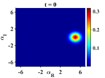
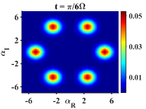
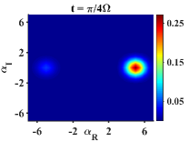
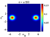
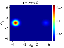
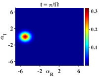
Figure 1: The evolution of multi-component cat-states for a system described by the nonlinear Hamiltonian eq. (5) where $k$ is any even number greater than $2$. The contour graphs show surface plots of $Q(\alpha)$ with $\alpha_{0}=5$. Plots are given for the times $t=0$, $t=\pi/6\Omega$, $t=\pi/4\Omega$, $t=\pi/2\Omega$, $t=3\pi/4\Omega$ and $t=\pi/\Omega$.

For the purpose of the Leggett-Garg tests, the times $t_{2}$ and $t_{3}$ will correspond to the system being in a cat-superposition state of some sort, where the amplitudes of the coherent states are well separated in phase space. For instance, Figure 1 shows such cat-superposition states at times $t=\pi/6\Omega$, $t=\pi/4\Omega$, $t=\pi/2\Omega$ and $t=3\pi/4\Omega$. We allow in general that the cat-states may be different at the different times. This deviates from the traditional Leggett-Garg test, where the system is in a superposition of the same two states at all times. The generalised Leggett-Garg inequalities, described in Section II, allow more flexibility to analyst Leggett-Garg violations.

IV Leggett-Garg violations for nonlinearity $k>2$, $k$ even

In this Section, we consider $k>2$ and $k$ even. We take $t_{1}=0$, when the system is prepared in a coherent state $|\alpha\rangle$ (where $\alpha$ is real) and consider the subsequent times $t_{2}=\pi/4\Omega$, $t_{3}=3\pi/4\Omega$. The analytic expression at time $t=\pi/4\Omega$ can be readily evaluated yurke-stoler . When $t=\pi/4\Omega$, $e^{-i\Phi_{n}}=\exp(-i\pi n^{k}/4)$. Therefore at $t=\pi/4\varOmega$ one has $e^{-i\varPhi_{n}}=(-1)^{n/2}$ when $n$ is even and $k=2$, and $e^{-i\varPhi_{n}}=1$ when $n$ is even and $k>2$. When $n$ is odd and $k$ even, one has $e^{-i\varPhi_{n}}=\frac{\sqrt{2}}{2}-i\frac{\sqrt{2}}{2}$ .

For our case of interest, when $k>2$ and $k$ is even, the state generated at time $t=\pi/4\Omega$ is

$$\left|\alpha,\pi/4\varOmega\right\rangle=\frac{1}{2}\{(1+e^{-i\pi/4})|\alpha\rangle+(1-e^{-i\pi/4})|-\alpha\rangle\}$$ (8)

At $t=3\pi/4\Omega$, the solution is

$$\left|\alpha,3\pi/4\varOmega\right\rangle=\frac{1}{2}\{(1-e^{-i\pi/4})|\alpha\rangle+(1+e^{-i\pi/4})|-\alpha\rangle\}$$ (9)

This compares with

$$\begin{array}[]{c}\frac{1}{\sqrt{2}}(e^{-i\frac{\pi}{4}}|\alpha\rangle+e^{+i\frac{\pi}{4}}|-\alpha\rangle)\end{array}$$ (10)

at the time $t=\pi/2\Omega$. The $Q$ functions for the states generated at the four times $t=0$, $\pi/4\Omega,$ $\pi/2\Omega$ and 3$\pi$/4$\Omega$  are plotted in Figure 2. Also plotted in Figure 3 is the value of the probability density $P(x)$ for a measurement $x$ on each of the states, where $\hat{x}={\color[rgb]{1,0,0}{\color[rgb]{0,0,1}{\color[rgb]{0,0,0}\frac{1}{\sqrt{2}}}}}(\hat{a}+\hat{a}^{\dagger})$. The calculations for $P(x)$ and the $Q$ function are outlined in the Appendix.

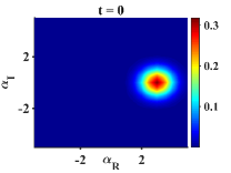
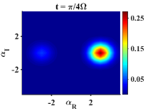
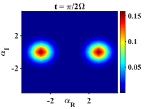
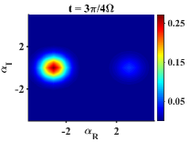
Figure 2: The evolution of two-component cat-states for a system described by the nonlinear Hamiltonian eq. (5) where $k$ is any even number greater than $2$. The contour graphs show surface plots of $Q(\alpha)$ with $\alpha_{0}=3$. The plots are given for the times $t=0$, $t=\pi/4\Omega$, $t=\pi/2\Omega$ and $t=3\pi/4\Omega$.

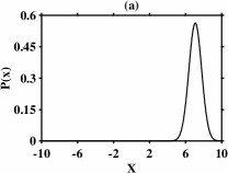
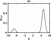
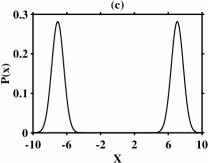
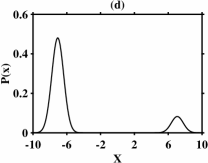
Figure 3: The evolution of two-component cat-states for a system described by the nonlinear Hamiltonian eq. (5) where $k$ is any even number greater than $2$. The graphs show plots of $P(x)$ with $\alpha=5$. The figures (a)-(d) give $P(x)$ at $t=0$, $t=\pi/4\Omega$, $t=\pi/2\Omega$, and $t=3\pi/4\Omega$ respectively.

We now evaluate the Leggett-Garg inequality (4) using $t_{1}=0$, $t_{2}=\pi/4\Omega$ and $t_{3}=3\pi/4\Omega$. Since $S_{1}=1$, we evaluate $\langle S_{1}S_{2}\rangle$ as $\langle S_{2}\rangle=P_{+}^{(2)}-P_{-}^{(2)}$, where $P_{+}^{(i)}=\int_{0}^{\infty}P(x)dx$ is the probability of result for $x$ being greater than or equal to $0$ at time $t_{i}$, and $P_{-}^{(i)}=\int_{-\infty}^{0}P(x)dx$ is the probability of result for $x$ being less than $0$ at time $t_{i}$. By integration, we find $P_{+}^{(2)}=0.8535$ and $P_{-}^{(2)}=0.1465$ ($\alpha\geq 2$). Therefore $\langle S_{1}S_{2}\rangle=0.7070$. Similarly, we see that $\langle S_{1}S_{3}\rangle=-\langle S_{1}S_{2}\rangle$ (refer Figure 2).

Determining $\langle S_{2}S_{3}\rangle$

We have evaluated the two-time moments $\langle S_{1}S_{2}\rangle$ and $\langle S_{1}S_{3}\rangle$ straightforwardly without consideration of any intermediate measurement that might be made at time $t_{2}$. This is justified for two reasons. First, in the Leggett-Garg derivation, such a measurement is required to be macroscopically noninvasive (refer Section VI). Also, the moments $\langle S_{1}S_{2}\rangle$ and $\langle S_{1}S_{3}\rangle$ are predicted to be a function of the time differences $t_{2}-t_{1}$ and $t_{3}-t_{1}$ respectively, which justifies the assumption of stationarity, that the two-time moments are invariant under time translation.

These considerations justify an approach that can be used to determine $\langle S_{2}S_{3}\rangle$. To evaluate $\langle S_{2}S_{3}\rangle$, we use the “measure and re-prepare” approach, discussed at the end of the Section II. Specifically, we will use the expression

$$\langle S_{2}S_{3}\rangle=P_{+}^{(2)}\langle S_{2}S_{3}\rangle_{+}+P_{-}^{(2)}\langle S_{2}S_{3}\rangle_{-}$$ (11)

where $P_{\pm}^{(2)}$ is the probability that the system at time $t_{2}$ has a positive or negative value for $x$. This probability can be measured experimentally. For sufficiently large $\alpha$, this probability is equal to the probability the system can be found to be in the $|\pm\alpha\rangle$ state. Here we denote $\langle S_{2}S_{3}\rangle_{+}$ as the average of $\langle S_{2}S_{3}\rangle$ given the state is prepared in the state $|\alpha\rangle$ at time $t_{2}$. Similarly, $\langle S_{2}S_{3}\rangle_{-}$ is the average of $S$ after a time $t$ given the state is prepared in the state $|-\alpha\rangle$ at time $t_{2}$. Recall from Section II that we define the two-time correlation as $\langle S_{2}S_{3}\rangle\equiv\langle S(t_{2})S(t_{3})\rangle$.

The expression (11) is justified if we assume the Leggett-Garg premises. At time $t_{2}$, the system is in a superposition of two states $|\psi_{1}\rangle$ and $|\psi_{2}\rangle$

$$|\psi\rangle=c_{-}|\psi_{1}\rangle+c_{+}|\psi_{2}\rangle$$ (12)

where $|\psi_{1}\rangle=|-\alpha\rangle$ and $|\psi_{2}\rangle=|\alpha\rangle$. Here $c_{-}$ and $c_{+}$ are probability amplitudes, where $P_{\pm}^{(2)}=|c_{\pm}|^{2}$ for large $\alpha$. The assumption of Leggett-Garg macro-realism is that the system is in one or the other of the states $|\psi_{1}\rangle$ and $|\psi_{2}\rangle$ at time $t_{2}$ (with probabilities $P_{+}^{(2)}$ and $P_{-}^{(2)}$ respectively). If we assume that at time $t_{2}$ the system was in state $|\alpha\rangle$, then this is the initial state for the calculation of $\langle S_{2}S_{3}\rangle$, which is then represented as $\langle S_{2}S_{3}\rangle_{+}$. We see that because $t_{3}-t_{2}=\pi/2\Omega$, if the system is indeed in the state $|\alpha\rangle$ at time $t_{2}$, then the system at the later time $t_{3}$ is in the symmetric state with equal probability for $x>0$ and $x<0$, as evident from Figures 2 and 3. Therefore $\langle S_{2}S_{3}\rangle_{+}=0$. Similarly, if we take that the system at time $t_{2}$ was in state $|-\alpha\rangle$, then we can show that $\langle S_{2}S_{3}\rangle_{-}=0$. Therefore $\langle S_{2}S_{3}\rangle=0$. Thus, we evaluate the Leggett-Garg term as

$${\color[rgb]{0,0,0}{\color[rgb]{0,0,0}\langle S_{1}S_{2}\rangle+\langle S_{2}S_{3}\rangle-\langle S_{1}S_{3}\rangle}=1.414}$$ (13)

This shows a violation of the Leggett-Garg inequality (4). The term “measure and re-prepare” is used to describe this technique because in principle, one can measure which state the system is in at time $t_{2}$, and then re-prepare that state to determine $\langle S_{2}S_{3}\rangle$. The assumption of stationarity however means that the moments $\langle S_{2}S_{3}\rangle_{\pm}$ (which are predicted to be dependent only on the time difference $t_{3}-t_{2}$) can be measured more conveniently in an independent experiment at any later or prior time.

V Leggett-Garg violations for nonlinearity $k=2$

For the case $k=2$, the evolution of the cat-states is different to the case with $k\neq 2$, $k$ even. We will consider other time intervals in order to obtain a violation of the Leggett-Garg inequality. The Appendix gives the analytical expressions for the states and the probabilities $P(x)$ at different times of evolution. The $Q$ functions for the states generated at a selection of different times are plotted in Figures 4 and 5.

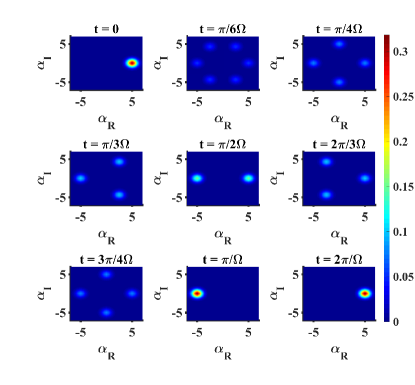
Figure 4: The evolution of multi-component cat-states for a system described by the nonlinear Hamiltonian eq. (5) where $k=2$. The contour graphs show surface plots of $Q(\alpha)$ with $\alpha_{0}=5$ for the times $t=0$, $t=\pi/6\Omega$, $t=\pi/4\Omega$, $t=\pi/3\Omega$, $t=\pi/2\Omega$, $t=2\pi/3\Omega$ and $t=3\pi/4\Omega$, $t=\pi/\Omega$ and $t=2\pi/\Omega$.

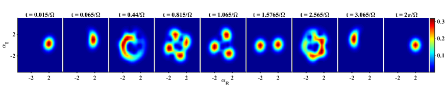
Figure 5: The time sequence showing the evolution of multi-component cat-states corresponding to the experiment of Kirchmair et al. collapse-revival-super-circuit . Here we take $\Omega$ to be negative, and $\alpha_{0}=2$ and $k=2$ for comparison with their reported results. We note the correspondence $\Omega=-\Omega_{K}/2$ where $\Omega_{K}$ is the nonlinearity defined by the Hamiltonian used in Ref. collapse-revival-super-circuit . The entire sequence was observed by them, except for the tri-cat state at $t=2\pi/3$. Here we show the surface plots of the $Q$ functions of the state at the given times.

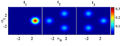
Figure 6: Surface plot of $Q(\alpha)$ with $\alpha_{0}=3$ and $k=2$ for the times $t=0$, $t=\pi/3\Omega$ and $t=2\pi/3\Omega$.

Specifically, we will consider the times $t_{1}=0$, $t_{2}=\pi/3\Omega$ and $t_{3}=2\pi/3\Omega$. This sequence for $\alpha=3$ is plotted in Figure 6. To give violation of the LG inequality, we select the values of $S_{i}$ differently at each of the times. This does not affect the derivation of the inequality, as shown in Section II. We define $S_{1}=+1$ if $x\geq 0$ and $S_{1}=-1$ otherwise. Similarly, we define $S_{2}=+1$ if $x\geq 0$ and $S_{2}=0$ otherwise. Finally, we define $S_{3}=-1$ if $x\leq 0$ and $S_{3}=0$ otherwise. Proceeding with the evaluation of the necessary moments, we find for $\alpha\geq 2$ on integrating $P(x)$ that $\begin{array}[]{ccc}\langle S_{1}S_{2}\rangle&=&\frac{2}{3}\end{array}$ and $\begin{array}[]{ccc}\langle S_{1}S_{3}\rangle&=&-\frac{2}{3}\end{array}$ (refer Table 1).

$t_{2}$	$t_{3}$
$\begin{array}[]{ccc}x\geq 0,&S_{2}=+1,&P_{+}=\frac{2}{3}\\ x<0,&S_{2}=0,&P_{-}=\frac{1}{3}\end{array}$	$\begin{array}[]{ccc}x>0,&S_{3}=0,&P_{+}=\frac{1}{3}\\ x\leq 0,&S_{3}=-1,&P_{-}=\frac{2}{3}\end{array}$

Table 1: Table showing the probabilities for outcomes at times $t_{2}$ and $t_{3}$ as evaluated for $\alpha\geq 2$.

To evaluate $\langle S_{2}S_{3}\rangle$, we follow the “measure and re-prepare” approach explained in Sections II and IV. The expansion of the state at time $t_{2}$ is given as

$$|\psi\rangle = i\frac{1}{\sqrt{3}}\left|-\alpha\right\rangle+\frac{1}{\sqrt{3}}\exp(-i\pi/6)\left|e^{i\pi/3}\alpha\right\rangle$$ (14)

$$+\frac{1}{\sqrt{3}}\exp(-i\pi/6)\left|e^{-i\pi/3}\alpha\right\rangle$$

This state is evident by the $Q$ function given in the plot of Figure 6. At time $t_{2}$, the system is thus in a superposition

$$|\psi\rangle=N_{0}(|\psi_{1}\rangle+|\psi_{2}\rangle)$$ (15)

where $|\psi_{1}\rangle=|-\alpha\rangle$ and

$$\left|\psi_{2}\right\rangle=N_{2}\{\left|e^{i\pi/3}\alpha\right\rangle+\left|e^{-i\pi/3}\alpha\right\rangle\}$$ (16)

The normalization constants are $\begin{array}[]{ccc}{\color[rgb]{0,0,0}N_{0}^{-2}}&{\color[rgb]{0,0,0}=}&{\color[rgb]{0,0,0}3\{1+2\exp(-\frac{3}{2}\alpha^{2})\cos(\frac{\sqrt{3}}{2}\alpha^{2})\}}\end{array}$ and ${\color[rgb]{0,0,0}N_{2}^{-2}=2\{1+\exp(-|\alpha|{}^{2}-\frac{1}{2}\alpha^{2})\cos(\frac{\sqrt{3}}{2}\alpha^{2})\}}$), noting the initial condition implies $\alpha$ real. The assumption of the macro-realism is that the system is in one or the other of the states $|\psi_{1}\rangle$ and $|\psi_{2}\rangle$ at time $t_{2}$. Using equation (11), we thus evaluate $\langle S_{2}S_{3}\rangle=P_{+}^{(2)}\langle S_{2}S_{3}\rangle_{+}+P_{-}^{(2)}\langle S_{2}S_{3}\rangle_{-}$ as given by Eq. (11), where $P_{-}^{(2)}$ is the probability the system is in state $|\psi_{1}\rangle$ at time $t_{2}$, and $\langle S_{2}S_{3}\rangle_{-}$ is the two-time moment given the system is in the state $|\psi{}_{1}\rangle$ at time $t_{2}$. Similarly, $P_{+}^{(2)}$ is the probability the system is in state $|\psi_{2}\rangle$ at time $t_{2}$, and $\langle S_{2}S_{3}\rangle_{+}$ is the two-time moment given the system is in the state $|\psi_{2}\rangle$ at time $t_{2}$. Following the “measure and re-prepare” procedure to evaluate $\langle S_{2}S_{3}\rangle_{-}$, we first assume the system was in $|\psi_{1}\rangle=|-\alpha\rangle$ at time $t_{2}=\pi/3\Omega$. We then evaluate what would have been the state at the later time $2\pi/3\Omega$, after evolution for a time $t=\pi/3\Omega$, with the initial state being $|\psi_{1}\rangle$. The final state in this case is the tri-cat state depicted in Figures 4 and Figure 6 at $t=2\pi/3\Omega$. From our definitions of $S_{2}$ and $S_{3}$ (Table 1), we see that $\langle S_{2}S_{3}\rangle_{-}=0$.

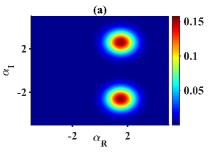
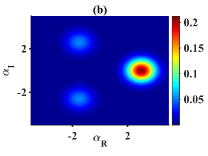
Figure 7: Surface plot of $Q(\alpha)$ with $\alpha_{0}=3$ and $k=2$. Figure (a) represents the initial state given by equation (16). Figure (b) is the time evolved state formed after a time $\pi/3\Omega$, as given by equation (LABEL:eq:state).

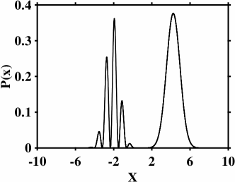
Figure 8: Plot of $P(x)$ for the state eq. (LABEL:eq:state) depicted in Figure 7b. The fringe pattern on the left is due to the superposition of the coherent states $|-e^{i\pi/3}\alpha\rangle$ and $|-e^{-i\pi/3}\alpha\rangle$. The probability of obtaining positive and negative results for $x$ are found on integration to be $P_{+}=0.6669$ and $P_{-}=0.3331$.

Continuing with the evaluation of $\langle S_{2}S_{3}\rangle$ based on the “measure and re-prepare” strategy, we next assume the system was in $|\psi_{2}\rangle$ at the time $t_{2}$. This state is depicted by its $Q$ function in Figure 7a. We then take this state to be the initial state for a calculation where the system evolves for a time $\pi/3\Omega$, to obtain the state that would have been generated at the time $t_{3}=2\pi/3\Omega$ with initial state $|\psi_{2}\rangle$. The state generated is

$$\left|\psi,\pi/3\right\rangle_{2} = N[\frac{2}{\sqrt{3}}e^{-i\pi/6}\left|\alpha\right\rangle$$

$$+\frac{1}{3}(2-e^{-i\pi/3})\{\left|-e^{i\pi/3}\alpha\right\rangle+\left|-e^{-i\pi/3}\alpha\right\rangle\}]$$

where $N^{-2}=2[1+\exp(-\frac{3}{2}\alpha^{2})\cos(\frac{\sqrt{3}}{2}\alpha^{2})]$. This state is depicted by its $Q$ function in Figure 7b. One evaluates the $P(x)$ for (LABEL:eq:state), to find

$$P(x) = \frac{N^{2}}{\sqrt{\pi}}\exp(-x^{2})\Bigl{\{}\frac{4}{3}\exp(2\sqrt{2}x\alpha-2\alpha{}^{2})$$ (18)

$$+\frac{4}{3}\exp(\frac{x\alpha}{\sqrt{2}}-\frac{5\alpha{}^{2}}{4})\cos(\frac{x\alpha\sqrt{6}}{2}+\frac{\alpha^{2}\sqrt{3}}{4})$$

$$+\frac{2}{3}\exp(-\sqrt{2}x\alpha-\frac{|\alpha|^{2}}{2})[1$$

$$\ \ \ \ \ \ \ \ \ +\cos(\sqrt{6}x\alpha+\frac{\alpha^{2}\sqrt{3}}{2})]\Bigl{\}}$$

as plotted in Figure 8. Evaluation of integrals gives probabilities of $P_{+}=2/3$ and $P_{-}=1/3$ for obtaining a positive and negative result for measurement of $x$ on this state (Figure 8). Thus

$$\langle S_{2}S_{3}\rangle_{+} = P_{+}\langle S_{3}\rangle_{+}+P_{-}\langle S_{3}\rangle_{-}=-\frac{1}{3}$$ (19)

Using eq. (11), we find $\langle S_{2}S_{3}\rangle=-\frac{2}{9}$. This implies

$$\langle S_{1}S_{2}\rangle-\langle S_{1}S_{3}\rangle+\langle S_{2}S_{3}\rangle=10/9$$ (20)

A violation of the Leggett-Garg inequality is obtained for the $k=2$ case.

VI Experimental strategy

Various experimental strategies can be used to demonstrate violation of the Leggett-Garg inequalities. These are documented in the literature lgexpphotonweak ; legggarg ; laura-lg-two-well ; jordan_kickedqndlg2 ; experiment-lg ; Mitchell ; stat-1zhou ; stat-2-neutrino ; small-systemlg ; emeryreview ; massiveosci ; NSTmunro . The inequality involves two-time correlation functions of three observables, $S_{1}$, $S_{2}$ and $S_{3}$, measured at three different times. A common strategy is to evaluate the two-time correlation moments by taking an ensemble average of an appropriate two-time moment with suitable initial states. As applied to this proposal, for two of the moments ($\langle S_{1}S_{2}\rangle$ and $\langle S_{1}S_{3}\rangle$) the initial state at the time $t_{1}$ is a coherent state, identical to the experiments collapse-revival-bec ; collapse-revival-super-circuit . The state formed at the intermediate time $t_{2}$ is a superposition of two states $\psi_{1}$ and $\psi_{2}$, which are well-separated and distinguishable by a measurement of a quadrature amplitude $\hat{x}$, as defined in Sections IV and V. The sign of the outcome for $\hat{x}$ determines the value of $S_{2}$. The moments obtained experimentally if this measurement $\hat{x}$ were performed can be evaluated from the experimentally determined $Q$ functions, given in Refs. collapse-revival-super-circuit . The validity of the evaluation of the moments for a test of macro-realism is based on the validity of the macro-realism premises. It is assumed that the system prior to any measurement will be in one of several macroscopically distinct states available to it. The value $S_{1}$ at time $t_{1}$ is known by preparation: the coherent state at time $t_{1}$ is prepared as $|\alpha\rangle$, which has a positive value for outcome $\hat{x}$ so that $S_{1}=1$. The value $S_{3}$ or $S_{2}$ (for evaluation of $\langle S_{1}S_{2}\rangle$ and $\langle S_{1}S_{3}\rangle$) is measurable by a projective measurement of $\hat{x}$ and hence of $S_{3}$ (or $S_{2}$): It is assumed this measurement correctly measures which of the states the system was in (prior to the measurement) to a macroscopic level of precision $-$ which is all that is necessary to determine $S_{i}$ prior to the measurement. In evaluating $\langle S_{1}S_{3}\rangle$, the measurement at time $t_{2}$ does not need to be made.

The moment $\langle S_{2}S_{3}\rangle$ is measurable using different strategies, including weak and ideal negative-result measurements, as discussed in Refs. lgexpphotonweak ; legggarg ; laura-lg-two-well ; jordan_kickedqndlg2 ; experiment-lg ; Mitchell ; stat-1zhou ; stat-2-neutrino ; small-systemlg ; emeryreview ; massiveosci ; NSTmunro . Here, we suggest a simple approach, as in Refs. NSTmunro ; stat-1zhou ; stat-2-neutrino ; laura-lg-two-well . It can be verified experimentally that at time $t_{2}$, the system is in the superposition of two macroscopically distinguishable states $\psi_{1}$ and $\psi_{2}$. The moment $\langle S_{2}S_{3}\rangle$ can be measured by first preparing the system in one state $\psi_{1}$ and then the other $\psi_{2}$, and measuring the moment $\langle S_{2}S_{3}\rangle$ for each case. The final moment is evaluated from the weighted average, assuming a stationarity, that the system evolves similarly under time translations stat-1zhou ; stat-2-neutrino . If the system is indeed in one or other state at time $t_{2}$ (as the first macro-realism premise implies), then the measured moment is justified to be the value $\langle S_{2}S_{3}\rangle$ that would be measured, if the ideal macroscopically noninvasive measurement could take place. A violation of the Leggett-Garg inequality observed with this approach then serves to invalidate the premise of macro-realism.

To carry out the evaluation of $\langle S_{2}S_{3}\rangle$ for $k=2$, we note that the first state $\psi_{1}$ of the superposition formed at time $t_{2}$ is a coherent state, which can be prepared and evolved to the tri-cat as in Ref collapse-revival-super-circuit . The second state $\psi_{2}$ of the superposition is itself a superposition, of two coherent states $\pi$ out of phase. This state $\psi_{2}$ can be re-prepared, up to a rotation in phase space, by evolving the coherent state for a time $t=\pi/2\Omega$, as illustrated in Figure 4. Evidence for the generation of this state $\psi_{2}$ is given in the BEC and superconducting circuit experiments of Refs. collapse-revival-bec ; collapse-revival-super-circuit . That this state is indeed generated can be established via tomography using the $Q$ function. In the anticipated experiment, the re-prepared state $\psi_{2}$ is then evolved for a time corresponding to $\pi/3\Omega$. The predicted state after this evolution is given in Figure 6b, from which the moments $\langle S_{2}S_{3}\rangle$ can be evaluated as described in Section V. The re-prepared state used here is different to $\psi_{2}$ by a rotation in phase space. One can justify that the measured correlation $\langle S_{2}S_{3}\rangle$ is unchanged, assuming the invariance of moments under rotations in phase space. Alternatively, one can experimentally obtain the rotated state, by rotating the initial coherent state.

VII Conclusion

In summary, we have derived generalizations of Leggett-Garg inequalities and demonstrated how the new inequalities can be used to test macro-realism for dynamical cat-states created by a nonlinearity. In particular, in Section V we demonstrate the feasibility of violating a Leggett-Garg inequality using a Kerr $\chi^{(3)}$ nonlinearity. This enables us to predict violation of Leggett-Garg inequalities for the experiments of Greiner et al. collapse-revival-bec and Kirchmair et al. collapse-revival-super-circuit . These experiments observe the collapse and revival of a coherent state over the necessary timescales.

Finally, we comment on loopholes and on the significance of the proposed Leggett-Garg test. First, we need to assume that the system at time $t_{1}$ is reliably prepared in the coherent state, and that the measurement at time $t_{3}$ accurately records the value of $S_{3}$ of the state of the system prior to measurement. The violation of the inequality would then negate that the system is in one or other of the macroscopically distinguishable states $\psi_{1}$ and $\psi_{2}$ at the time $t_{2}$ (or similarly at time $t_{3}$). This is because a system in a classical mixture $\rho_{mix}$ of these states at these times would satisfy the Leggett-Garg premises. (This is understood because the system is in one of the two macroscopically distinguishable states, and a measurement can be constructed that leaves these states unchanged). Hence if the system is in a classical mixture $\rho_{mix}$ of the two states, one could not generate a violation of the inequalities. The violation of the Leggett-Garg inequality thus gives a demonstration of a mesoscopic quantum coherence.

It could be argued that the failure of the mixture $\rho_{mix}$ is also exemplified by the observation of the revival of the final coherent state as observed in the experiments of Refs. collapse-revival-super-circuit ; collapse-revival-bec , since a classical mixture $\rho_{mix}$ would not give a such a revival. However, this latter argument does not rule out that the system might be describable as another mixture consistent with the macro-realism premises in a theory alternative to quantum mechanics. In this respect, the violation of the Leggett-Garg inequality, which does not rely on quantum mechanics, is designed to give a stronger conclusion.

Extra assumptions also exist for the Leggett-Garg test however, which create loopholes. The proposed strategy relies on the preparation of the states $\psi_{1}$ and $\psi_{2}$ at the time $t_{2}$ for the evaluation of the $\langle S_{2}S_{3}\rangle$, and we thus assume the state regenerated for the later measurement is the actual $\psi_{i}$. The objective of the Leggett-Garg inequality however is to falsify the premises of macro-realism for all theories, not only quantum mechanics. For this there is a potential loophole, since it could not be excluded that for an alternative theory, the system at time $t_{2}$ is in a state microscopically different to the state $\psi_{1}$ or $\psi_{2}$. These states may be minimally disturbed by the measurement performed at $t_{2}$, and it might be argued that this minimal disturbance may generate after evolution a macroscopic change to the state (and hence to $S_{3}$) at the later time $t_{3}.$ This would not affect the justification of the evaluation of $\langle S_{2}S_{3}\rangle$ or $\langle S_{1}S_{3}\rangle$. However, for the evaluation of $\langle S_{2}S_{3}\rangle$ one could then not exclude that a small difference to the state measured at $t_{2}$ results in a macroscopic difference to the outcome at the time $t_{3}$. To eliminate such a loophole, one is left with the difficult task to regenerate all states that are microscopically different to $\psi_{1}$ and $\psi_{2}$, and demonstrate that the evolution from time $t_{2}$ to $t_{3}$ does not change the value of $S$ measured at $t_{3}$. Alternatively, one can seek to perform the Leggett-Garg test using an ideal negative-result measurement or a weak measurement legggarg ; emeryreview .

Appendix

Coherent state expansion of states

In the problems treated, we consider the initial state of the system to be a coherent state $\left|\psi,t=0\right\rangle=\left|\alpha\right\rangle$ where $\alpha$ is real. In some cases, it is well-known that the state created at a later time can be written as a superposition of a finite number of distinct coherent states. A summary of some such examples in given in the Table 2. Important for this paper is that the state $|\psi,t=\pi/3\Omega\rangle$ (for $k=2$) is a superposition of three coherent states $\left|-\alpha\right\rangle$, $\left|e^{i\pi/3}\alpha\right\rangle$ and $\left|e^{-i\pi/3}\alpha\right\rangle$. That this is so is suggested by the plot of the $Q$ function, given in Figure 4. A simple analysis allows us to evaluate the probability amplitudes, given as $|\psi,t=\pi/3\Omega\rangle=A|-\alpha\rangle+B|e^{i\pi/3}\alpha\rangle+C|e^{-i\pi/3}\alpha\rangle$ . One can write the state at this time as

$$\left|\alpha,\pi/3\varOmega\right\rangle = e^{-|\alpha|^{2}/2}\underset{n}{\sum}A(-1)^{n}\alpha^{n}\frac{1}{\sqrt{n!}}\left|n\right\rangle$$

$$+e^{-|\alpha|^{2}/2}\underset{n}{\sum}B(e^{i\pi/3})^{n}\alpha^{n}\frac{1}{\sqrt{n!}}\left|n\right\rangle$$

$$+e^{-|\alpha|^{2}/2}\underset{n}{\sum}C(e^{-i\pi/3})^{n}\alpha^{n}\frac{1}{\sqrt{n!}}\left|n\right\rangle$$

$$= e^{-|\alpha|^{2}/2}\underset{n}{\sum}\exp(-i\pi n^{2}/3)\alpha^{n}\frac{1}{\sqrt{n!}}\left|n\right\rangle$$

Evaluation of the amplitudes $A$, $B$ and $C$ is done by simultaneously solving for the coefficients, where $n=0,1,2,...$. By solving we can write the wavefunction as in eq. (14).

Evaluation of $P(x)$ and the $Q$ function

We evaluate $P(x)$ using the expression $P(x_{\theta})$ for the probability measurement: $P(x_{\theta})=|\langle x_{\theta}|\psi\rangle|^{2}$ where $\hat{x_{\theta}}=(e^{i\theta}\hat{\alpha}+e^{-i\theta}\hat{a^{\dagger}})\sqrt{2}$. The generalized position representation $\psi_{\alpha,t}(x)=\left\langle x|\alpha,t\right\rangle$ can be written as yurke-stoler

$$\psi_{\alpha}(x_{\theta})=\frac{1}{\pi^{1/4}}\exp(-\frac{x^{2}}{2}+\frac{2x|\alpha|e^{i(\theta+\phi)}}{\sqrt{2}}-\frac{|\alpha|^{2}e^{2i(\theta+\phi)}}{2}-\frac{|\alpha|^{2}}{2})$$

where $\alpha=|\alpha|e^{i\phi}$. By using the expression for $\theta=0$, we see that $P(x)=\frac{1}{\pi^{1/2}}\exp(-x^{2}+2\sqrt{2}x\alpha-2|\alpha|^{2})$. A summary of the position probability distributions $P(x)$ evaluated for the various times is given in the Table 3.

We also evaluate the Husimi Q Husimi-Q representation defined as $Q(\alpha)=\langle\alpha|\rho|\alpha\rangle/\pi=\langle\alpha|\psi\rangle\langle\psi|\alpha\rangle/\pi=|\langle\alpha|\psi\rangle|^{2}/\pi$. At $t=0$, we take $\psi=|\alpha_{0}\rangle$. Then

$$Q(\alpha)=\frac{1}{\pi}\exp(-|\alpha|^{2}-|\alpha_{0}|^{2}+\alpha_{0}(\alpha^{*}+\alpha))$$

where we have considered $\alpha_{0}$ is real. The remaining functions are calculated using that the inner product of two coherent states is $\langle\alpha|\beta\rangle=\exp(-\frac{|\alpha|^{2}}{2}-\frac{|\beta|^{2}}{2}+\alpha^{*}\beta)$. A summary of the functions $Q(\alpha)$ evaluated for various times is given in the table 4 below.

	$\psi_{\alpha}$	relevant $k$
$t=0$	$\left|\alpha\right\rangle$	all $k$
$t=\pi/8\Omega$	$\begin{array}[]{c}{\normalcolor\frac{\sqrt{2}}{4}e^{-i\pi/8}\{|e^{i\pi/4}\alpha\rangle-|-e^{i\pi/4}\alpha\rangle+}|e^{-i\pi/4}\alpha\rangle-|-e^{-i\pi/4}\alpha\rangle\}\\ +\frac{1}{4}\{(1-i)(|\alpha\rangle+|-\alpha\rangle)+(1+i)(|i\alpha\rangle+|-i\alpha\rangle)\}\end{array}$	$k=2$
$t=\pi/4\Omega$	$\begin{array}[]{c}\frac{1}{2}\{|-i\alpha\rangle+|i\alpha\rangle+e^{-i\pi/4}|\alpha\rangle-e^{-i\pi/4}|-\alpha\rangle\}\\ \\ \end{array}$	$\begin{array}[]{c}k=2\\ \\ \end{array}$
	$\frac{1}{2}\{(1+e^{-i\pi/4})|\alpha\rangle+(1-e^{-i\pi/4})|-\alpha\rangle\}$	$k>2$, $k$ even
$t=\pi/3\Omega$	$i\frac{1}{\sqrt{3}}\left|-\alpha\right\rangle+\frac{1}{\sqrt{3}}\exp(-i\pi/6)\left|e^{i\pi/3}\alpha\right\rangle+\frac{1}{\sqrt{3}}\exp(-i\pi/6)\left|e^{-i\pi/3}\alpha\right\rangle$	$k=2$
$t=3\pi/8\Omega$	$\begin{array}[]{c}{\normalcolor\frac{\sqrt{2}}{4}e^{-i3\pi/8}\{|e^{i\pi/4}\alpha\rangle-|-e^{i\pi/4}\alpha\rangle+}|e^{-i\pi/4}\alpha\rangle-|-e^{-i\pi/4}\alpha\rangle\}\\ +\frac{1}{4}\{(1+i)(|\alpha\rangle+|-\alpha\rangle)+(1-i)(|i\alpha\rangle+|-i\alpha\rangle)\}\end{array}$	$k=2$
$t=\pi/2\Omega$	$\begin{array}[]{c}\frac{1}{\sqrt{2}}(e^{-i\frac{\pi}{4}}|\alpha\rangle+e^{+i\frac{\pi}{4}}|-\alpha\rangle)\\ \\ \end{array}$	$k$ even
	$\frac{1}{2}(|\alpha\rangle+|-\alpha\rangle+|-i\alpha\rangle-|i\alpha\rangle)$	$k$ odd
$t=5\pi/8\Omega$	$\begin{array}[]{c}{\normalcolor\frac{\sqrt{2}}{4}e^{-i5\pi/8}\{|e^{i\pi/4}\alpha\rangle-|-e^{i\pi/4}\alpha\rangle+}|e^{-i\pi/4}\alpha\rangle-|-e^{-i\pi/4}\alpha\rangle\}\\ +\frac{1}{4}\{(1-i)(|\alpha\rangle+|-\alpha\rangle)+(1+i)(|i\alpha\rangle+|-i\alpha\rangle)\}\end{array}$	$k=2$
$t=2\pi/3\Omega$	$\frac{1-2e^{i\pi/3}}{3}\left|\alpha\right\rangle+\frac{1}{\sqrt{3}}e^{i\pi/6}\left|-e^{i\pi/3}\alpha\right\rangle+\frac{1}{\sqrt{3}}e^{i\pi/6}\left|-e^{-i\pi/3}\alpha\right\rangle)$	$k=2$
$t=3\pi/4\Omega$	$\begin{array}[]{c}\frac{1}{2}\{|-i\alpha\rangle+|i\alpha\rangle-e^{+i\pi/4}|\alpha\rangle+e^{+i\pi/4}|-\alpha\rangle\}\\ \\ \end{array}$	$\begin{array}[]{c}k=2\\ \\ \end{array}$
	$\frac{1}{2}\{(1-e^{+i\pi/4})|\alpha\rangle+(1+e^{+i\pi/4})|-\alpha\rangle\}$	$k>2$, $k$ even
$t=7\pi/8\Omega$	$\begin{array}[]{c}{\normalcolor\frac{\sqrt{2}}{4}e^{-i7\pi/8}\{|e^{i\pi/4}\alpha\rangle-|-e^{i\pi/4}\alpha\rangle+}|e^{-i\pi/4}\alpha\rangle-|-e^{-i\pi/4}\alpha\rangle\}\\ +\frac{1}{4}\{(1+i)(|\alpha\rangle+|-\alpha\rangle)+(1-i)(|i\alpha\rangle+|-i\alpha\rangle)\}\end{array}$	$k=2$
$t=\pi/\Omega$	$\left|-\alpha\right\rangle$	all $k$

Table 2: Summary of the multi-component cat-states formed at different times, for different $k$.

	$P(x)$	$k$
$t=0$	$\begin{array}[]{c}\frac{1}{\pi^{1/2}}\exp(-x^{2}+2\sqrt{2}x\alpha-2|\alpha|^{2})\end{array}$	all $k$
$t=\pi/4\Omega$	$\begin{array}[]{c}\frac{1}{2}\frac{1}{\pi^{1/2}}\exp(-x^{2}-|\alpha|^{2})\{2\sinh(|\alpha|^{2})+\exp(-|\alpha|^{2})\cosh(2\sqrt{2}x\alpha)\\ +\exp(|\alpha|^{2})\cos(2\sqrt{2}x\alpha)+2\sqrt{2}\cos(\sqrt{2}x\alpha)\sinh(\sqrt{2}x\alpha)\}\end{array}$	$k=2$
	$\begin{array}[]{c}\begin{array}[]{c}\frac{1}{\pi^{1/2}}\exp(-x^{2}-2|\alpha|^{2})\{\cosh(2\sqrt{2}x\alpha)+\frac{1}{\sqrt{2}}\sinh(2\sqrt{2}x\alpha)\}\end{array}\end{array}$	$k>2$, $k$ even
$t=\pi/3\Omega$	$\begin{array}[]{c}\frac{1}{3}\frac{1}{\pi^{1/2}}\exp(-x^{2})\{\exp(-2\sqrt{2}x\alpha-2\alpha^{2})+2\exp(\sqrt{2}x\alpha-\alpha{}^{2}/2)\\ -2\exp(-\frac{\sqrt{2}}{2}x\alpha-5\alpha^{2}/4)\cos(\frac{\sqrt{6}}{2}x\alpha-\frac{\sqrt{3}}{4}\alpha^{2})\\ +2\exp(\sqrt{2}x\alpha-\alpha^{2}/2)\cos(\sqrt{6}x\alpha-\frac{\sqrt{3}}{2}\alpha^{2})\}\end{array}$	$k=2$
$t=\pi/2\Omega$	$\frac{1}{\pi^{1/2}}\exp(-x^{2}-2|\alpha|^{2})\cosh(2\sqrt{2}xa)$	$k$ even
$t=3\pi/4\Omega$	$\begin{array}[]{c}\frac{1}{2}\frac{1}{\pi^{1/2}}\exp(-x^{2}-|\alpha|^{2})\{2\sinh(|\alpha|^{2})+\exp(-|\alpha|^{2})\cosh(2\sqrt{2}x\alpha)\\ +\exp(|\alpha|^{2})\cos(2\sqrt{2}x\alpha)-2\sqrt{2}\cos(\sqrt{2}x\alpha)\sinh(\sqrt{2}x\alpha)\}\end{array}$	$k=2$
	$\begin{array}[]{c}\frac{1}{\pi^{1/2}}\exp(-x^{2}-2|\alpha|^{2})\{\cosh(2\sqrt{2}x\alpha)\\ -\frac{1}{\sqrt{2}}\sinh(2\sqrt{2}x\alpha)\}\end{array}$	$k>2$, $k$ even
$t=\pi/\Omega$	$\begin{array}[]{c}\frac{1}{\pi^{1/2}}\exp(-x^{2}-2\sqrt{2}x\alpha-2|\alpha|^{2})\end{array})$	all $k$

Table 3: Summary of the probability distributions $P(x)$ for various $t$ and $k$.

$t$	$Q(\alpha)$	$k$
$t=0$	$\frac{1}{\pi}\exp(-|\alpha|^{2}-|\alpha_{0}|^{2}+\alpha_{0}(\alpha^{*}+\alpha))$	all $k$
$t=\pi/4\Omega$	$\begin{array}[]{c}\frac{1}{\pi}\exp(-|\alpha|^{2}-|\alpha_{0}|^{2})\{\cos(\alpha^{*}\alpha_{0})+e^{-i\pi/4}\sinh(\alpha^{*}\alpha_{0})\}\\ \times\{\cos(\alpha_{0}\alpha)+e^{+i\pi/4}\sinh(\alpha_{0}\alpha)\}\end{array}$	$k=2$
	$\begin{array}[]{c}\frac{1}{\pi}\exp(-|\alpha|^{2}-|\alpha_{0}|^{2})\{\cosh(\alpha\alpha_{0}+\alpha^{*}\alpha_{0})\\ +\frac{1}{\sqrt{2}}\sinh(\alpha\alpha_{0}+\alpha^{*}\alpha_{0})+i\frac{1}{\sqrt{2}}\sinh(\alpha\alpha_{0}-\alpha^{*}\alpha_{0})\}\end{array}$	$k>2$, $k$ even
$t=\pi/3\Omega$	$\begin{array}[]{c}\frac{1}{3}\frac{1}{\pi}\exp(-|\alpha_{0}|{}^{2}-|\alpha|^{2}+\frac{1}{2}\alpha_{0}\alpha^{*}+\frac{1}{2}\alpha_{0}\alpha)\{\exp(-\frac{3}{2}\alpha\alpha_{0})+2ie^{i\pi/6}\cos(\frac{\sqrt{3}}{2}\alpha\alpha_{0})\}\\ \times\{\exp(-\frac{3}{2}\alpha^{*}\alpha_{0})-2ie^{-i\pi/6}\cos(\frac{\sqrt{3}}{2}\alpha^{*}\alpha_{0})\}\end{array}$	$k=2$
$t=\pi/2\Omega$	$\begin{array}[]{c}\frac{1}{\pi}\exp(-|\alpha|^{2}-|\alpha_{0}|^{2})[\cosh(\alpha^{*}\alpha_{0}+\alpha\alpha_{0})-i\sinh(\alpha^{*}\alpha_{0}-\alpha\alpha_{0})]\end{array}$	$k$ even
$t=3\pi/4\Omega$	$\begin{array}[]{c}\frac{1}{\pi}\exp(-|\alpha|^{2}-|\alpha_{0}|^{2})\{\cos(\alpha^{*}\alpha_{0})-e^{+i\pi/4}\sinh(\alpha^{*}\alpha_{0})\}\\ \times\{\cos(\alpha_{0}\alpha)-e^{-i\pi/4}\sinh(\alpha_{0}\alpha)\}\end{array}$	$k=2$
	$\begin{array}[]{c}\frac{1}{\pi}\exp(-|\alpha|^{2}-|\alpha_{0}|^{2})\{\cosh(\alpha^{*}\alpha_{0}+\alpha\alpha_{0})\\ -\frac{1}{\sqrt{2}}\sinh(\alpha^{*}\alpha_{0}+\alpha\alpha_{0})-i\frac{1}{\sqrt{2}}\sinh(\alpha^{*}\alpha_{0}-\alpha\alpha_{0})\}\end{array}$	$k>2$, $k$ even
$t=\pi/\Omega$	$\frac{1}{\pi}\exp(-|\alpha|^{2}-|\alpha_{0}|^{2}-\alpha_{0}(\alpha^{*}+\alpha))$	all $k$

Table 4: $Q(\alpha)$ functions evaluated for various times and $k$.

References

- (1) E. Schroedinger, “The Present Status of Quantum Mechanics”, Die Naturwissenschaften. 23, 807 (1935).
- (2) Florian Fröwis, Pavel Sekatski, Wolfgang Dür, Nicolas Gisin, and Nicolas Sangouard, “Macroscopic quantum states: measures, fragility, and implementations”, Rev. Mod. Phys. 90, 025004 (2018)
- (3) S. Haroche, “Nobel Lecture: Controlling photons in a box and exploring the quantum to classical boundary”, Rev. Mod. Phys. 85, 1083 (2013). D. J. Wineland, “Nobel Lecture: Superposition, entanglement, and raising Schrödinger’s cat”, Rev. Mod. Phys. 85, 1103 (2013).
- (4) B. Vlastakis et al., Science 342, 607 (2013). C. Wang et al., Science 352, 1087 (2016).
- (5) Markus Greiner, Olaf Mandel, Theodor Hånsch and Immanuel Bloch, “Collapse and revival of the matter wave field of a Bose-Einstein condensate”, Nature 419, 51 (2002).
- (6) Gerhard Kirchmair et al., “Observation of the quantum state collapse and revival due to a single-photon Kerr effect”, Nature 495, 205 (2013).
- (7) A. Leggett and A. Garg, “Quantum mechanics versus macroscopic realism: is the flux there when nobody looks?”, Phys. Rev. Lett. 54, 857 (1985).
- (8) J. S. Bell, “On the Einstein-Podolsky-Rosen Paradox”, Physics 1, 195 (1964).
- (9) C. Emary, N. Lambert and F. Nori, “Leggett-Garg inequalities”, Rep. Prog. Phys 77, 016001 (2014).
- (10) J. Dressel et al., ”Experimental Violation of Two-Party Leggett-Garg Inequalities with Semiweak Measurements”, Phys. Rev. Lett. 106, 040402 (2011). J. S. Xu et al., “Experimental violation of the Leggett-Garg inequality under decoherence”, Scientific Report 1, 101 (2011). V. Athalye, S. S. Roy, and T. S. Mahesh, “Investigation of the Leggett-Garg Inequality for Precessing Nuclear Spins”, Phys. Rev. Lett. 107, 130402 (2011). A. M. Souza, I. S. Oliveira and R. S. Sarthour, “A scattering quantum circuit for measuring Bell’s time inequality: a nuclear magnetic resonance demonstration using maximally mixed states”, New J. Phys. 13 053023 (2011). G. Waldherr et al.,“Violation of a Temporal Bell Inequality for Single Spins in a Diamond Defect Center”, Phys.Rev. Lett. 107, 090401 (2011). H. Katiyar et al., “Violation of entropic Leggett-Garg inequality in nuclear spins”, Phys. Rev. A 87, 052102 (2013). R. E. George et al., “Opening up three quantum boxes causes classically undetectable wavefunction collapse”, Proc. Natl Acad. Sci. 110 3777 (2013). G. C. Knee et al., “Violation of a Leggett–Garg inequality with ideal non-invasive measurements”, Nature Commun. 3, 606 (2012).
- (11) M. E. Goggin, et al., “Violation of the Leggett-Garg inequality with weak measurements of photons”, Proc. Natl. Acad. Sci. 108, 1256 (2011).
- (12) Z. Q. Zhou, S. Huelga, C-F Li and G-C Guo, “Experimental Detection of Quantum Coherent Evolution through the Violation of Leggett-Garg-Type Inequalities”, Phys. Rev. Lett. 115, 113002 (2015).
- (13) J. A. Formaggio et al., “Violation of the Leggett-Garg Inequality in Neutrino Oscillations”, Phys. Rev. Lett. 117, 050402 (2016).
- (14) A. Palacios-Laloy, F. Mallet, F. Nguyen, P. Bertet, Denis Vion, Daniel Esteve and Alexander N. Korotkov, “Experimental violation of a Bell’s inequality in time with weak measurement”, Nature Phys. 6, 442 (2010).
- (15) C. Robens, W. Alt, D. Meschede, C. Emary, and A. Alberti, “Ideal Negative Measurements in Quantum Walks Disprove Theories Based on Classical Trajectories”, Phys. Rev. X 5, 011003 (2015).
- (16) G. C. Knee, K. Kakuyanagi, M.-C. Yeh, Y. Matsuzaki, H. Toida, H. Yamaguchi, S. Saito, A. J. Leggett and W. J. Munro, “A strict experimental test of macroscopic realism in a superconducting flux qubit”, Nat. Commun. 7, 13253 (2016).
- (17) A. N. Jordan, A. N. Korotkov, and M. Buttiker, “Leggett-Garg Inequality with a Kicked Quantum Pump”, Phys. Rev. Lett. 97, 026805 (2006).
- (18) A. Asadian, C. Brukner and P. Rabl, “Probing Macroscopic Realism via Ramsey Correlation Measurements”, Phys. Rev. Lett. 112, 190402 (2014).
- (19) C. Budroni, G. Vitagliano, G. Colangelo, R. J. Sewell, O. Gühne, G. Tóth, and M. W. Mitchell, “Quantum Nondemolition Measurement Enables Macroscopic Leggett-Garg Tests”, Phys. Rev. Lett. 115, 200403 (2015).
- (20) B. Opanchuk, L. Rosales-Zárate, R. Y. Teh, and M. D. Reid, “Quantifying the mesoscopic quantum coherence of approximate NOON states and spin-squeezed two-mode Bose-Einstein condensates”, Phys. Rev. A 94, 062125 (2016);
- (21) L. Rosales-Zárate, B. Opanchuk, Q. Y. He, and M. D. Reid, “Leggett-Garg tests of macrorealism for bosonic systems including two-well Bose-Einstein condensates and atom interferometers”, Phys. Rev. A 97, 042114 (2018).
- (22) G. Milburn and C. Holmes, “Dissipative quantum and classical Liouville mechanics of the anharmonic oscillator”, Phys. Rev. Lett. 56, 2237 (1986).
- (23) B. Yurke and D. Stoler, “Generating quantum mechanical superpositions of macroscopically distinguishable states via amplitude dispersion”, Phys. Rev. Lett. 57, 13 (1986).
- (24) E. Wright, D. Walls and J. Garrison, “Collapses and revivals of Bose-Einstein condensates formed in small atomic samples”, Phys. Rev. Lett. 77, 2158 (1996).
- (25) E. A. Rojas Gonz´alez, A. Borne, B. Boulanger, J. A. Levenson, and K. Bencheikh, “Continuous variable triple-photon states quantum entanglement”, Phys. Rev. Lett. 120, 043601 (2018).
- (26) Y. Aharonov, D. Albert and L. Vaidmann, “How the result of a measurement of a component of the spin of a spin-1/2 particle can turn out to be 100”, Phys. Rev. Lett. 60, 1351 (1988). N. S. Williams, A. N. Jordan, “Weak Values and the Leggett-Garg Inequality in Solid-State Qubits”, Phys. Rev. Lett. 100, 026804 (2008).
- (27) J. Dressel, M. Malik, F. M. Miatto, A. N. Jordan and R. W. Boyd, “Understanding quantum weak values: Basics and applications”, Rev. Mod. Phys. 86, 307 (2014). T. C. White et al., “Preserving entanglement during weak measurement demonstrated with a violation of the Bell-Leggett-Garg inequality”, NPJ Quantum Inf. 2, 15022 (2016). B. L. Higgins, M. S. Palsson, G. Y. Xiang, H. M. Wiseman, and G. J. Pryde, “Using weak values to experimentally determine negative probabilities in a two-photon state with Bell correlations”, Phys. Rev. A 91, 012113 (2015).
- (28) L. Rosales-Zárate, B. Opanchuk, and M. D. Reid, “Weak measurements and quantum weak values for NOON states”, Phys. Rev. A 97, 032123 (2018).
- (29) Clauser and Shimony, “Bell’s theorem: experimental tests and implications”, Rep. Prog. Phys. 41, 1881 (1978).
- (30) Kôdi Husimi (1940). "Some Formal Properties of the Density Matrix", Proc. Phys. Math. Soc. Jpn. 22: 264-314.