Three-dimensional mixing and light curves: constraints on the progenitor of supernova 1987A

With the same method as used previously, we investigate neutrino-driven explosions of a larger sample of blue supergiant models. The blue supergiants were evolved as single-star progenitors. The larger sample includes three new presupernova stars. The results are compared with light-curve observations of the peculiar type IIP supernova 1987A (SN 1987A). The explosions were modeled in 3D with the neutrino-hydrodynamics code Prometheus-HOTB, and light-curve calculations were performed in spherical symmetry with the radiation-hydrodynamics code Crab, starting at a stage of nearly homologous expansion. Our results confirm the basic findings of the previous work: 3D neutrino-driven explosions with SN 1987A-like energies synthesize an amount of ⁵⁶Ni that is consistent with the radioactive tail of the light curve. Moreover, the models mix hydrogen inward to minimum velocities below 400 km s^-1 as required by spectral observations and a 3D analysis of molecular hydrogen in SN 1987A. Hydrodynamic simulations with the new progenitor models, which possess smaller radii than the older ones, show much better agreement between calculated and observed light curves in the initial luminosity peak and during the first 20 days. A set of explosions with similar energies demonstrated that a high growth factor of Rayleigh-Taylor instabilities at the (C+O)/He composition interface combined with a weak interaction of fast Rayleigh-Taylor plumes, where the reverse shock occurs below the He/H interface, provides a sufficient condition for efficient outward mixing of ⁵⁶Ni into the hydrogen envelope. This condition is realized to the required extent only in one of the older stellar models, which yielded a maximum velocity of around 3000 km s^-1 for the bulk of ejected ⁵⁶Ni, but failed to reproduce the helium-core mass of 6 $M_{\sun}$ inferred from the absolute luminosity of the presupernova star. We conclude that none of the single-star progenitor models proposed for SN 1987A to date satisfies all constraints set by observations.

1 Introduction

The explosion of the blue supergiant (BSG) Sanduleak $-69^{\circ}202$ in the Large Magellanic Cloud (LMC) as the peculiar type II plateau supernova (SN) 1987A stimulated not only activity in its observation from radio wavelengths to gamma rays, but also the further development in the theory of the evolution of massive stars, the simulation of explosion mechanisms, and the modeling of light curves and spectra. This well-observed object displayed a number of intriguing observational features (Arnett et al. 1989), two of which are interesting in the context of this paper. First, the progenitor of SN 1987A was a compact star, but not a red supergiant (RSG). Second, SN 1987A exhibited clear observational evidence for macroscopic mixing that must have occurred during the explosion.

Over the past three decades, the relative compactness of the BSG progenitor Sanduleak $-69^{\circ}202$ of SN 1987A has been a puzzling problem for the theory of the evolution of massive stars, and no consensus has been reached on its origin so far. A single-star scenario to fit the observed properties of the progenitor with evolutionary calculations requires either a metal-deficient composition similar to the LMC (Arnett 1987; Hillebrandt et al. 1987), a modification of convective mixing through rotation-induced meridional circulation in the star during its evolution (Weiss et al. 1988), a restricted semiconvective diffusion (Woosley et al. 1988; Langer 1991), or both mass loss and convective mixing (Saio et al. 1988). Binary stellar evolution invoking a strong accretion of matter from the companion star (Podsiadlowski & Joss 1989) or a merger of the companion star with the primary RSG (Hillebrandt & Meyer 1989; Podsiadlowski et al. 1990, 2007; Menon & Heger 2017) can also explain the properties of the SN 1987A progenitor. Podsiadlowski (1992) showed, however, that only binary scenario models are able to fit all available observational and theoretical constraints.

Observational evidence for mixing of radioactive ⁵⁶Ni and hydrogen in the ejected envelope exists not only at early times, but also at late times (see Utrobin et al. 2015, for details). During $20-100$ days after the explosion, the H$\alpha$ profile exhibited a striking fine structure called “Bochum event” (Hanuschik & Dachs 1987; Phillips & Heathcote 1989). At day 410, a unique high-velocity feature with a radial velocity of about $+3900$ km s^-1 was found in the infrared emission lines of [Fe ii] and was interpreted as a fast-moving iron clump (Haas et al. 1990). Utrobin et al. (1995) analyzed the H$\alpha$ profile at the Bochum event phase and identified this high-velocity feature with a fast ⁵⁶Ni clump that was moving at an absolute velocity of 4700 km s^-1 and had a mass of $\sim$10${}^{-3}\,M_{\sun}$. The bulk of radioactive ⁵⁶Ni had a maximum velocity of $\sim$3000 km s^-1, as inferred from the infrared emission lines of [Ni ii] and [Fe ii] at day 640 (Colgan et al. 1994). Chugai (1991) studied the profiles of hydrogen emission lines at day 350 and found that the slowest-moving hydrogen-rich matter had a velocity of $\sim$600 km s^-1. In turn, Kozma & Fransson (1998) analyzed the H$\alpha$ profile taken at day 804 and argued that hydrogen was mixed down into the innermost ejecta to velocities of $\leq 700$ km s^-1. Maguire et al. (2012) revisited the line profiles during the nebular phase and showed that they are peaked in shape, suggesting that mixing of the elements including hydrogen must have occurred in the ejecta down to zero velocity. Reconstructing a 3D view of molecular hydrogen in SN 1987A, Larsson et al. (2019) found that the lowest observed velocities of molecular hydrogen are in the range of 400 to 800 km s^-1. Thus, the presence of hydrogen in the innermost layers of the ejecta is confirmed by observational data of SN 1987A.

These comprehensive observational data unambiguously demonstrate that the envelope of the pre-SN was substantially mixed during the explosion. In the framework of the standard paradigm of neutrino-powered explosions in 2D geometry, Kifonidis et al. (2006) demonstrated that massive ⁵⁶Ni-dominated clumps can be mixed deep into the helium shell and even into the hydrogen layer of the disrupted star, with terminal velocities of up to $\sim$3000 km s^-1. In turn, hydrogen can be mixed at the He/H composition interface downward in velocity space to about 500 km s^-1. Later 3D hydrodynamic simulations of neutrino-driven explosions for SN 1987A (Hammer et al. 2010; Wongwathanarat et al. 2010b; Müller et al. 2012; Wongwathanarat et al. 2013, 2015) confirmed the basic results of the 2D simulations concerning the mixing of radioactive ⁵⁶Ni and hydrogen. Kifonidis et al. (2006) and Wongwathanarat et al. (2015) found that the amount of outward ⁵⁶Ni mixing and inward hydrogen mixing is sensitive to the structure of the helium core and the He/H composition interface.

Using this sensitivity, Utrobin et al. (2015) studied the dependence of explosion properties on the structure of four BSG progenitors for the first time in the framework of the neutrino-driven explosion mechanism. The authors compared their light curves with observations of SN 1987A. The considered pre-SN models, 3D explosion simulations, and light-curve calculations explain the basic observational features of SN 1987A. However, only one hydrodynamic model reproduces the width of the broad maximum of the observed light curve promisingly well, and no model matches the observational features connected to the pre-SN structure of the outer stellar layers. All progenitor models have radii that are too large to reproduce the observed narrow initial luminosity peak, and the structure of their outer layers does not match the observed light curve during the first 30–40 days.

We therefore explore three new BSG models for Sanduleak $-69^{\circ}202$ that have smaller radii than the old models, some of which were discussed in Sukhbold et al. (2016). Applying the self-consistent approach developed in Utrobin et al. (2015) to these three new BSG models, we find that the mixing that occurs during the explosion plays a crucial role in constraining the helium-core properties of the progenitor.

We begin in Sect. 2 with a brief description of the pre-SN models and the numerical approach. In Sect. 3 we present and analyze our results, and compare them with SN 1987A observations. We conclude in Sect. 4 with a summary and discussion of our findings. In Appendix A we discuss the role of 3D macroscopic mixing in light-curve modeling of ordinary and peculiar type IIP SNe.

2 Model overview and numerical approach

Our overview of pre-SN models includes seven (three new and four previously used) available models obtained in the scenario of single-star evolution. The numerical approach we follow in this work is identical to that presented in Utrobin et al. (2015). It consists of three steps: 3D simulations of the neutrino-driven explosion, mapping 3D simulation results to 1D, and hydrodynamic light-curve modeling. We briefly review each step in the following subsections.

2.1 Presupernova models

Table 1: Presupernova models for blue supergiants.

Model	$R_{\mathrm{pSN}}$	$M_{\mathrm{CO}}^{\,\mathrm{core}}$	$M_{\mathrm{He}}^{\,\mathrm{core}}$	$M_{\mathrm{pSN}}$	$M_{\mathrm{ZAMS}}$	$Y_{\mathrm{surf}}$	$Z_{\mathrm{surf}}$	Rot.	Ref.
	$(R_{\sun})$	$(M_{\sun})$					$(10^{-2})$
W16	28.8	2.57	6.55	15.36	16	0.521	0.50	Yes	1
W18r	41.9	2.67	6.65	17.09	18	0.453	0.50	Yes	–
W18x	30.4	2.12	5.13	17.56	18	0.281	0.60	Yes	1
B15	56.1	1.64	4.05	15.02	15.02	0.230	0.34	No	2
W18	46.8	3.06	7.40	16.92	18.0	0.515	0.50	Yes	1
W20	64.2	2.33	5.79	19.38	20.10	0.256	0.56	No	3
N20	47.9	3.75	5.98	16.27	$\sim$20.0	0.435	0.50	No	4

(1) Sukhbold et al. (2016); (2) Woosley et al. (1988); (3) Woosley et al. (1997); (4) Shigeyama & Nomoto (1990).

Most pre-SN models of our study are described in detail in Sukhbold et al. (2016). Here we only provide a brief overview of their basic properties (Table 1). Model B15 (model W15 in the nomenclature of Sukhbold et al. (2016)) was evolved by Woosley et al. (1988) from the main sequence to the precollapse stage. This single 15 $M_{\sun}$ star has a reduced metallicity. When evolved with restricted semiconvection and without mass loss, it produced a BSG star. Its luminosity, related to its helium-core mass of 4.05 $M_{\sun}$, is too low compared to the observational data of Sanduleak $-69^{\circ}202$, which require a single star to have a helium-core mass of about 6 $M_{\sun}$ (Saio et al. 1988; Woosley et al. 1988).

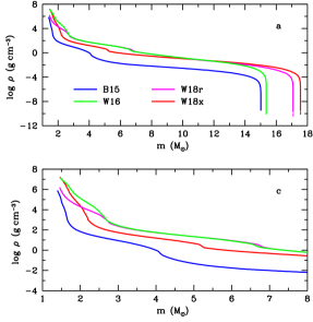
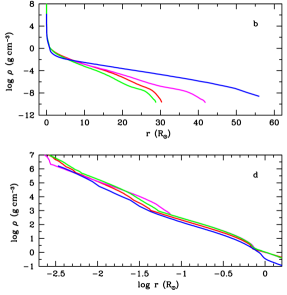
Figure 1: Density distribution as a function of interior mass for the whole star (a) and the inner region of 8 $M_{\sun}$ (c), and as a function of radius for the whole star (b) and the inner region of 1 $R_{\sun}$ (d) in the pre-SN models B15, W16, W18r, and W18x. The central collapsing core that is integrated into the neutron star is omitted.

We here study models W16, W18, and W18x of the BSG progenitor models presented in Sukhbold et al. (2016). Model W18 was evolved with reduced metallicity and restricted semiconvection, like model B15, and with a substantial amount of rotation and mass loss. Rotation increases the helium-core mass to 7.4 $M_{\sun}$ and also stirs more helium into the hydrogen envelope, enriching its surface mass fraction to 0.515. A higher helium-core mass implies a higher luminosity, somewhat above the observed limit for Sanduleak $-69^{\circ}202$. Two other models, which are similar to model W18, illustrate some sensitivities: model W16 is identical to model W18, except for its different mass and rotation rate; model W18x is slightly different in input physics and has less total angular momentum on the main sequence. The angular momenta on the main sequence for models W16, W18, and W18x are $(2.7,3.1,\mathrm{and}\ 2.3)\times 10^{52}$ erg s, respectively.

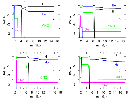
Figure 2: Mass fractions of hydrogen (black), helium (blue), CNO-group elements (green), and iron-group elements (magenta) in the pre-SN models B15 (a), W16 (b), W18r (c), and W18x (d).

Model W18r is an 18 $M_{\sun}$ progenitor evolved with rotation and angular momentum transport, including magnetic torques (Spruit 2002; Heger et al. 2005). The total initial angular momentum on the main sequence was $3.1\times 10^{52}$ erg s, which was reduced by transport and mass loss to $2.4\times 10^{51}$ erg s at death. The initial mass was 18.0 $M_{\sun}$, and the final mass was 17.09 $M_{\sun}$, with a helium core of 6.65 $M_{\sun}$ and a CO core of 2.67 $M_{\sun}$. The initial composition was taken to be representative of the subsolar metallicity of the LMC. Hydrogen, helium, carbon, nitrogen, and oxygen had mass fractions of 0.745, 0.250, $5.2\times 10^{-4}$, $1.2\times 10^{-4}$, and $2.5\times 10^{-3}$, respectively. We note that this initial composition was used in the other models W16, W18, W18x, and W20 as well. These may not be the best modern values, but the total abundance of CNO-group elements is reduced by about a factor of three compared to solar. This weakens the hydrogen-burning shell and helps to make a BSG star.

Model W20 was evolved by Woosley et al. (1997), again including mass loss, and using the revised opacities of Rogers & Iglesias (1992) and Iglesias & Rogers (1996), which were also applied in all other models except for B15 (where recalculation with the new opacities did not yield any significant differences). Its helium-core mass of 5.79 $M_{\sun}$, the corresponding luminosity, and radius agree well with observations of Sanduleak $-69^{\circ}202$. The hydrogen envelope is not enriched in helium, whose surface mass fraction is 0.256.

In all model progenitors described above, nuclear burning was followed using the usual 19 isotope “approx” network until oxygen depletion and the 128 isotope quasi-equilibrium network thereafter (Weaver et al. 1978). In addition to this standard reaction network, in model W18r, nucleosynthesis and gradual changes in the electron mole number were followed using an adaptive network (Rauscher et al. 2002) that contained about 1500 isotopes at the end.

Model N20 was constructed by Shigeyama & Nomoto (1990) by combining the pre-SN helium core of 6 $M_{\sun}$ evolved by Nomoto & Hashimoto (1988) with the hydrogen envelope that was independently calculated by Saio et al. (1988). Both the helium core and the hydrogen envelope were defined to satisfy observational constraints from Sanduleak $-69^{\circ}202$. This model is therefore somewhat artificial and is not an evolutionary pre-SN model that is evolved continuously from the main sequence onward.

It is noteworthy that the low mass of the CO core relative to the helium-core mass has proven important for obtaining a BSG pre-SN solution. This was achieved in the Kepler code by limiting semiconvection to a relatively low efficiency and neglecting overshoot mixing. The progenitor models B15, W16, W18, W18r, W18x, and W20 that were evolved in this approach to a BSG configuration have the mass ratio of the CO core to the helium core in the range of 0.392 to 0.414, while model N20 originally constructed to obtain a RSG solution has this ratio of 0.627 (Table 1).

We already analyzed the four models B15, W18, W20, and N20 in a previous paper (Utrobin et al. 2015) and now focus on the three new models W16, W18r, and W18x; we use model B15 as a reference case. The new models have different helium-core masses close to the observationally required value of 6 $M_{\sun}$ (Table 1; Figs. 1a and c), which allows us to study the sensitivity of the amount of outward ⁵⁶Ni mixing and inward hydrogen mixing to the structure of the helium core and the He/H composition interface. In addition, these models also differ in their density distributions (Fig. 1) and chemical compositions (Fig. 2). All new models have smaller surface radii than the older models (Table 1).

2.2 Numerical methods

Our 3D neutrino-driven explosion simulations begin shortly after the stellar core has collapsed and a newly formed SN shock wave has propagated to a mass coordinate of approximately 1.25 $M_{\sun}$ inside the iron core. The evolution during core collapse and core bounce were computed in spherical symmetry and were provided to us by Sukhbold et al. (2016). After mapping the 1D post-bounce data onto a 3D grid, the 3D calculations were carried out with the explicit finite-volume Eulerian multifluid hydrodynamics code Prometheus (Fryxell et al. 1991; Müller et al. 1991a, b). Details of the physics modules implemented into the Prometheus code and our numerical setup have been described in Wongwathanarat et al. (2013) for neutrino-driven explosion simulations and in Wongwathanarat et al. (2015) for simulations of the late-time evolution from approximately 1.3 s after core bounce onward. Nevertheless, we briefly summarize the input physics and numerical methods employed by our code as follows.

The Prometheus code uses a dimensionally split version of the piecewise parabolic method (Colella & Woodward 1984) to solve the multidimensional hydrodynamic equations. A fast and efficient Riemann solver for real gases (Colella & Glaz 1985) is used to compute numerical fluxes at cell boundaries. Inside grid cells, where a strong shock wave is present, we recompute the inter-cell fluxes using an approximate Riemann solver (Liou 1996) to prevent numerical artifacts known as the odd-even decoupling (Quirk 1994). The yin-yang overlapping grid (Kageyama & Sato 2004), implemented into Prometheus as in Wongwathanarat et al. (2010a), is employed for efficient spatial discretization of the computational domain. Newtonian self-gravity is taken into account by solving Poisson’s equation in its integral form, using an expansion into spherical harmonics (Müller & Steinmetz 1995). In addition, a general relativistic correction of the monopole term of the gravitational potential is applied during the explosion simulations following Scheck et al. (2006) and Arcones et al. (2007).

To model the explosive nucleosynthesis approximately, a small $\alpha$-chain reaction network, similar to the network described in Kifonidis et al. (2003), is solved. In order to unambiguously determine the inward mixing of hydrogen, free protons, which are produced when neutrino-heated matter freezes out from nuclear statistical equilibrium, are distinguished from hydrogen originating from the hydrogen-rich stellar envelope by tagging them as different species in our multicomponent treatment of the stellar plasma.

The revival of the stalled SN shock and the explosion are triggered by imposing a suitable value of the neutrino luminosities at an inner radial grid boundary located at an enclosed mass of 1.1 $M_{\sun}$, well inside the neutrinosphere. Outside this boundary, which shrinks with time to mimic the contraction of the proto-neutron star, we model neutrino-matter interactions by solving the neutrino radiation transport equation in a “ray-by-ray” manner and in the gray approximation as described in Scheck et al. (2006). The explosion energy of the model is determined by the imposed isotropic neutrino luminosity, whose temporal evolution we prescribe as well, and by the accretion luminosity that results from the progenitor-dependent mass accretion rate and the gravitational potential of the contracting neutron star.

Our 3D calculations terminate at approximately one day after the explosion when the SN shock wave has swept through the entire progenitor star. The further time evolution of the SN outburst beyond one day is modeled in one dimension. To this end, we compute angle-averaged profiles of hydrodynamic quantities and chemical abundances of the 3D flow at chosen times and interpolate these profiles onto the Lagrangian (mass) grid used in the 1D simulations. The resulting data are the initial conditions for the hydrodynamic modeling of the SN outburst. Our 3D simulations of neutrino-driven explosions eliminate the need to initiate the explosion by a supersonic piston or a thermal and/or kinetic bomb.

The numerical modeling of the SN outbursts employs the implicit Lagrangian radiation hydrodynamics code Crab (Utrobin 2004, 2007). It integrates the set of spherically symmetric hydrodynamic equations including self-gravity, and a radiation transfer equation in the gray approximation (e.g., Mihalas & Mihalas 1984). The time-dependent radiative transfer equation, written in a comoving frame of reference to an accuracy of order $v/c$ ($v$ is the fluid velocity, and $c$ is the speed of light), is solved as a system of equations for the zeroth and first angular moments of the nonequilibrium radiation intensity. This system of two moment equations is closed by calculating a variable Eddington factor directly, taking into account scattering of radiation in the SN ejecta. In the inner optically thick layers of the ejecta, the diffusion of equilibrium radiation is treated in the approximation of radiative heat conduction. The resulting set of equations is discretized spatially using the method of lines (e.g., Hairer et al. 1993; Hairer & Wanner 1996). The energy deposition of gamma rays with energies of about 1 MeV from the decay chain ⁵⁶Ni $\to^{56}$Co $\to^{56}$Fe is determined by solving the corresponding gamma-ray transport. The equation of state, the mean opacities, and the thermal emission coefficient are calculated taking non-LTE and nonthermal effects into account. In addition, the contribution of spectral lines to the opacity in a medium expanding with a velocity gradient is estimated using the generalized formula of Castor et al. (1975). We refer to Utrobin et al. (2015) and references therein for details of the numerical setup.

3 Results

Table 2: Basic properties of the 3D hydrodynamic models.

Model	m$M_{\mathrm{NS}}$	m$M_{\mathrm{env}}$	m$E_{\mathrm{exp}}$	m$M_{\mathrm{Ni}}^{\,\mathrm{min}}$	e$M_{\mathrm{Ni}}^{\,\mathrm{max}}$	m$M_{\mathrm{Ni}}^{\,\mathrm{i}}$	m$M_{\mathrm{Ni}}^{\,\mathrm{f}}$	m$v_{\mathrm{Ni}}^{\,\mathrm{bulk}}$	m$\langle v\rangle_{\mathrm{Ni}}^{\mathrm{tail}}$	m$v_{\mathrm{H}}^{\,\mathrm{mix}}$	m$\delta M_{\mathrm{H}}^{\,\mathrm{mix}}$	m$\delta M_{\mathrm{p}}^{\,\mathrm{free}}$	m$\Delta M_{\mathrm{H}}^{\mathrm{2000}}$	m$t_{\mathrm{map}}$	m$t_{\mathrm{SB}}$m
	$(M_{\sun})$		(B)	$(10^{-2}\,M_{\sun})$				($10^{3}$ km s-1)			$(10^{-2}\,M_{\sun})$		$(M_{\sun})$	($10^{3}$ s)
W16-1	2.08	13.25	0.88	2.47	5.07	5.07	3.47	1.43	1.52	1.27	9.74	1.32	0.694	89.28	3.39
W16-2	1.90	13.45	1.16	3.03	8.00	8.00	6.92	2.37	2.50	1.48	12.52	2.32	0.322	88.82	3.03
W16-3	1.66	13.69	1.48	4.06	12.43	8.67	7.85	2.71	2.95	1.85	4.42	3.32	0.060	88.49	2.66
W16-4	1.58	13.78	1.81	4.70	15.46	8.47	7.97	2.84	3.02	2.01	6.91	3.87	0.037	88.26	2.44
W18r-1	1.43	15.65	1.05	1.77	7.01	7.01	6.33	1.00	1.04	1.42	1.62	2.54	0.868	90.47	4.72
W18r-2	1.35	15.73	1.31	2.46	9.35	7.90	7.57	1.15	1.20	1.61	1.61	3.07	0.462	89.77	4.30
W18r-3	1.31	15.77	1.59	2.93	11.35	7.88	7.69	1.43	1.52	1.78	1.84	3.31	0.146	89.08	3.94
W18r-4	1.27	15.80	1.91	3.12	13.18	7.78	7.76	1.68	1.75	1.98	2.59	3.41	0.039	89.26	3.62
W18x-1	1.57	15.97	1.21	2.79	9.06	9.06	7.02	2.36	2.47	1.20	7.87	2.30	1.354	89.45	3.72
W18x-2	1.52	16.03	1.45	3.89	12.21	8.43	7.55	2.46	2.85	1.36	5.40	2.78	0.847	89.13	3.43
B15-2	1.25	14.20	1.40	3.07	9.28	7.29	7.25	3.37	3.50	0.27	15.32	1.92	0.922	61.22	6.20
W18	1.47	15.45	1.36	2.91	11.00	8.38	7.62	1.38	1.47	1.76	1.69	3.11	0.168	55.20	4.26
W20	1.49	17.87	1.45	3.23	11.18	7.72	7.48	1.39	1.49	1.31	4.21	3.35	1.312	61.24	6.66
N20-P	1.46	14.69	1.67	3.97	11.71	7.65	7.58	1.61	1.79	0.19	22.66	3.61	0.353	56.86	5.40

We performed ten 3D neutrino-driven explosion simulations with the three new pre-SN models W16, W18r, and W18x (Table 1) as initial data. In Table 2 we list some basic properties of these 3D hydrodynamic models that we extracted at the end of the simulations. For completeness, we also list the properties of the four old models B15-2, W18, W20, and N20-P that have been analyzed in Utrobin et al. (2015). We define the explosion energy, $E_{\mathrm{exp}}$, as the sum of the total (i.e., internal plus kinetic plus gravitational) energy of all grid cells at the mapping moment. Throughout this paper, we employ the energy unit $1\,\mathrm{bethe}=1\,\mathrm{B}=10^{51}$ erg.

3.1 Production of ⁵⁶Ni in neutrino-driven simulations

Our 3D supernova simulations are characterized by the explosion energy, the total amount of radioactive ⁵⁶Ni, and the amount of macroscopic mixing of ⁵⁶Ni and hydrogen-rich matter occurring during the SN explosion (Table 2). To follow the explosive nucleosynthesis, we solved a small $\alpha$-chain reaction network and are therefore unable to determine the mass fraction of ⁵⁶Ni in the tracer matter very accurately. A possible overall production of radioactive ⁵⁶Ni falls in between the minimum and maximum values: the mass of ⁵⁶Ni produced directly by our $\alpha$-chain reaction network, $M_{\mathrm{Ni}}^{\,\mathrm{min}}$, and the aggregate mass of directly produced ⁵⁶Ni and tracer nucleus, $M_{\mathrm{Ni}}^{\,\mathrm{max}}$ (see Utrobin et al. 2015, for details)). Two sets of 3D models $\{$W16-1, W16-2, W16-3, W16-4$\}$ and $\{$W18r-1, W18r-2, W18r-3, W18r-4$\}$ show that the production of radioactive ⁵⁶Ni is proportional to the explosion energy (Table 2); this confirms the results of Utrobin et al. (2015). Moreover, the 3D models B15-2, W16-3, W18, W18r-2, W18x-2, W20, and N20-P comply with the finding that the ⁵⁶Ni production is mostly dependent on the explosion energy (which is similar in all cases of this group of models), whereas the detailed properties of the pre-SN, that is, different helium-core masses ranging from 4 to 7.4 $M_{\sun}$ (Table 1), different density structures (Fig. 1; Utrobin et al. 2015, Fig. 1), and different chemical compositions (Fig. 2; Utrobin et al. 2015, Fig. 2), play a less important role.

3.2 Mixing in neutrino-driven explosion simulations

Figure 3: Time-integrated Rayleigh-Taylor growth factors vs. enclosed mass for the 1D hydrodynamic models B15, W16, W18, W18r, W18x, W20, and N20 at the given times. The vertical red and blue lines denote the mass coordinates of the (C+O)/He and He/H composition interfaces, respectively. These interfaces are Rayleigh-Taylor unstable after the passage of the SN shock.

In order to picture turbulent mixing in 3D simulations, we outline the development of neutrino-driven explosions after core bounce (see, e.g., Wongwathanarat et al. 2015, for details). The value of the explosion energy is determined by the isotropic neutrino luminosity at the inner grid boundary, its prescribed temporal evolution, and the accretion luminosity. Neutrino heating causes buoyant bubbles to form in the convectively unstable layer that builds up within the neutrino-heating region between the gain radius and the stalled SN shock. These high-entropy bubbles start to rise, grow, and merge. As a result, the delayed, neutrino-driven explosion sets in, supported by convective overturn and large-scale aspherical shock oscillations caused by the standing accretion shock instability (SASI).

After the SN shock wave has been launched by neutrino heating, the further evolution of the explosion depends strongly on the density profile of the progenitor. The shock decelerates when it encounters a density profile that falls off less steeply than $\rho\sim r^{-3}$, and it accelerates for density profiles that are steeper (Sedov 1959). At the locations of the Si/O, (C+O)/He, and He/H composition interfaces (Fig. 2), the value of $\rho r^{3}$ varies nonmonotonically with radius such that the shock velocity increases when the shock approaches a composition interface and decreases after the shock has crossed the interface. A deceleration of the shock causes a density inversion in the post-shock flow, which means that a dense shell forms. Such shells at the locations of the composition interfaces are subject to Rayleigh-Taylor instabilities because they are characterized by density and pressure gradients of opposite signs (Chevalier 1976).

To compare the relative strength of the growth of Rayleigh-Taylor instabilities in different progenitor models, we performed an additional set of 1D neutrino-driven explosion simulations for all progenitor stars, including those already presented in Utrobin et al. (2015). Our 1D modeling approach is the same as in our 3D simulations. This set of 1D models develops approximately the same explosion energy of 1.4 B. To qualitatively analyze these instabilities in our 3D simulations, we computed the linear Rayleigh-Taylor growth rate in these 1D models for an incompressible fluid given by (Bandiera 1984; Benz & Thielemann 1990; Müller et al. 1991b)

$$\sigma_{\mathrm{RT}}=\sqrt{-{\partial P\over\partial r}{\partial\rho\over\partial r}}\;.$$ (1)

The growth factor for the time-dependent perturbation $\xi$ increases with time $t$ as (Hattori et al. 1986)

$${\xi\over\xi_{0}}(t)=\exp\left(\int_{0}^{t}\sigma_{\mathrm{RT}}(\tau)\,d\tau\right)\;,$$ (2)

where $\xi_{0}$ is the amplitude of an initial perturbation at fixed Lagrangian mass coordinate.

Figure 3 displays the time-integrated Rayleigh-Taylor growth factors as functions of enclosed mass in our 1D models for each of the progenitors (Table 1) at times long after the shock breakout. The growth factors in the Rayleigh-Taylor unstable layer near the (C+O)/He composition interface greatly vary between the different progenitors, with model B15 showing the largest growth factor. On the other hand, the Rayleigh-Taylor growth factors at the He/H interface show less variation and differ only by approximately one order of magnitude between progenitors, except for model N20, which exhibits a particularly large growth factor. It is interesting to note here again that the helium core and the hydrogen envelope of the progenitor model N20 were evolved separately in two stellar evolution calculations by Nomoto & Hashimoto (1988) and Saio et al. (1988). Thus, the large growth factor at the He/H interface observed in this model might not be physical. It should also be emphasized that the results of the linear perturbation theory presented in Fig. 3 can only provide qualitative information on the relative strength of the expected growth of Rayleigh-Taylor instabilities in different layers of the progenitor star. In realistic 3D simulations, the instabilities will quickly enter the nonlinear regime. Nevertheless, the results from the linear analysis prove to be useful for a qualitative understanding of differences in the extent of mixing of ⁵⁶Ni in different progenitors (see Sect. 3.3).

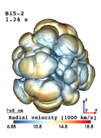
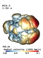
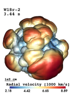
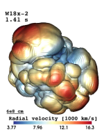
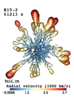
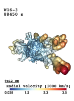
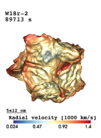
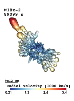
Figure 4: Morphology of radioactive ⁵⁶Ni-rich matter produced by explosive burning in shock-heated ejecta. The snapshots display isosurfaces where the mass fraction of ⁵⁶Ni plus the neutron-rich tracer nucleus equals $3\%$. The isosurfaces are shown for four 3D models at two different epochs: shortly before the SN shock crosses the (C+O)/He composition interface in the progenitor star (upper row), and long after the shock breakout (lower row). In the top left corner of each panel, we give the name of the model and the post-bounce time of the snapshot. The colors give the radial velocity on the isosurface, and the color-coding is defined at the bottom of each panel. The size of the displayed volume and of the clumps can be estimated from the yardsticks given in the lower left corner of each panel. There is a striking difference between model B15-2 and the other three models in the final morphology of the ⁵⁶Ni-rich ejecta, which arises from their specific progenitor structures and the influence of the latter on the unsteady SN shock propagation.

The SN shock wave first crosses the Si/O interface and then reaches the (C+O)/He interface, at which time the maximum speed of the bulk mass of ⁵⁶Ni-rich matter, $v_{\mathrm{Ni}}^{\mathrm{CO}}$, is spread over a wide range from 7850 to 19 850 km s^-1 (Table 3; Fig. 4, upper row), depending on the progenitor, for models with comparable explosion energies (Table 2). When the shock wave crosses the (C+O)/He interface and then enters the helium layer, a reverse shock forms. After the main shock has passed the He/H interface, the evolution resembles the situation after crossing of the (C+O)/He interface, and another reverse shock forms below the He/H interface. By this time, the fastest Rayleigh-Taylor plumes (a few in the case of model B15-2, and one plume in the case of models W16-3 and W18x-2) remain close to the main shock and avoid interaction with the strong reverse shock. Therefore, they penetrate the hydrogen envelope with high velocities, in stark contrast to the situation in the other models W18, W18r-2, W20, and N20-P. As a result, the maximum velocities of iron-group nuclei and other elements decrease only slightly at late times, and the fastest ⁵⁶Ni-rich clumps move with velocities of $\approx$3200 to $\approx$3700 km s^-1 in models W18x-2, W16-3, and B15-2 (Fig. 4, lower row; Fig. 5; Utrobin et al. 2015, Fig. 3, lower row; Fig. 10). In contrast, the other mushrooms penetrate the reverse shock and move supersonically relative to the ambient medium, dissipating a large portion of their kinetic energy in bow shocks and strong acoustic waves, and forming an almost spherical distribution with velocities between $\approx$1100 and $\approx$2100 km s^-1 in models W18r-2, W18, W20, and N20-P (Fig. 4, lower row; Fig. 5; Utrobin et al. 2015, Fig. 3, lower row; Fig. 10). This striking difference in the morphology of the ⁵⁶Ni-rich ejecta was discussed extensively in previous works of Kifonidis et al. (2003, 2006).

The Rayleigh-Taylor instabilities and the global deformation of the main shock give rise to substantial inward mixing of hydrogen. The aspherical shock deposits large amounts of vorticity into the layer at the He/H interface and thus induces mixing of hydrogen-rich matter down into the He shell. To estimate the real extent of hydrogen mixing, we distinguish between hydrogen-rich matter (mass $\delta M_{\mathrm{H}}^{\,\mathrm{mix}}$) mixed from the hydrogen envelope into the He shell and free protons (mass $\delta M_{\mathrm{p}}^{\,\mathrm{free}}$) left uncombined in the neutrino-heated ejecta originating from the SN explosion (Table 2, Fig. 5).

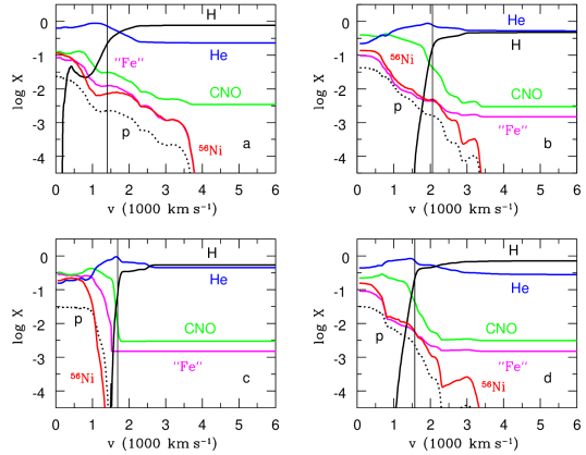
Figure 5: Mass fractions of hydrogen (solid black), free protons (dotted black), helium (blue), CNO-group elements (green), iron-group elements except for ⁵⁶Ni (magenta), and radioactive ⁵⁶Ni (red) as functions of velocity at day 50 in models B15-2 (a), W16-3 (b), W18r-2 (c), and W18x-2 (d). Thin vertical lines indicate ejecta velocities at the location of the outer edge of the pre-SN helium core.

In Table 2 we present some global properties of mixing induced by the 3D neutrino-driven explosions in the ejecta. To characterize mixing of radioactive ⁵⁶Ni in radial velocity space, we divided the ⁵⁶Ni-rich ejecta into two components: a slow-moving bulk of ⁵⁶Ni containing $99\%$ of the total ⁵⁶Ni mass, and a fast-moving ⁵⁶Ni tail containing the remaining $1\%$. This division is motivated by the observational evidence for a fast ⁵⁶Ni clump of $\sim$10${}^{-3}\,M_{\sun}$ in SN 1987A (Utrobin et al. 1995). We determined the maximum velocity of the bulk component, $v_{\mathrm{Ni}}^{\,\mathrm{bulk}}$, and the mean velocity of the tail component, $\langle v\rangle_{\mathrm{Ni}}^{\mathrm{tail}}$. On the other hand, inward mixing of hydrogen-rich matter may be measured by the mass of hydrogen mixed into the He shell and its minimum velocity, $v_{\mathrm{H}}^{\,\mathrm{mix}}$. We also evaluated the total mass of free protons produced in the neutrino-heated matter and left over in the SN ejecta. Finally, it is instructive to determine the mass of hydrogen confined to the inner layers ejected with velocities lower than 2000 km s^-1, $\Delta M_{\mathrm{H}}^{\mathrm{2000}}$, which was estimated by Kozma & Fransson (1998).

Two sets of new models $\{$W16-1, W16-2, W16-3, W16-4$\}$, $\{$W18r-1, W18r-2, W18r-3, W18r-4$\}$ (Table 2), and a set of old models B15-1, B15-2, B15-3 (Utrobin et al. 2015) demonstrate that the greater the explosion energy, the more intense the outward mixing of radioactive ⁵⁶Ni in velocity space. In turn, the mass of hydrogen mixed into the He shell in the two sets of new models does not correlate with the explosion energy, while its minimum velocity grows with the explosion energy (Table 2). The finding regarding the mass of hydrogen mixed into the He shell has no simple explanation because the large-scale mixing is the result of a complex sequence of hydrodynamic instabilities at the composition interfaces (cf. Wongwathanarat et al. 2015).

The mass of free protons left over in the neutrino-heated ejecta from the 3D explosion simulations increases with the explosion energy (Table 2). Their distributions in velocity space are very similar to those of radioactive ⁵⁶Ni (Fig. 5) because the origins of the two nucleosynthesis components are similar. The extent of free proton mixing may be measured by the maximum velocity of the bulk mass of ⁵⁶Ni. The smoothness of the resulting distribution of hydrogen matter is determined by overlapping the distributions of hydrogen mixed into the He shell and these free protons. The degree of this overlapping correlates with the ratio of $v_{\mathrm{Ni}}^{\,\mathrm{bulk}}$ to $v_{\mathrm{H}}^{\,\mathrm{mix}}$: the greater this ratio, the smoother the distribution of hydrogen. It turns out that the degree of overlapping is not sensitive to the explosion energy, as two sets of new models show in Table 2. This reflects the fact that the smoothness of the hydrogen distribution inside the He shell depends mainly on the properties of the progenitor. It is noteworthy that in our hydrodynamic models, the minimum velocity of free protons is lower than 400 km s^-1, while hydrogen-rich matter mixed into the He shell expands with velocities exceeding 1200 km s^-1, except for models B15-2 and N20-P.

Macroscopic mixing of radioactive ⁵⁶Ni outward and hydrogen-rich matter inward continues until the ejecta reach homologous expansion. Utrobin et al. (2015) showed that the bulk of ⁵⁶Ni containing $99\%$ of the total ⁵⁶Ni mass expands almost homologously in the four old models B15-2, W18, W20, and N20-P already by the time when we map our 3D hydrodynamic data onto the 1D Lagrangian grid. The same holds for the three new models W16-3, W18r-2, and W18x-2. Hence, we consider our 3D neutrino-driven simulations mapped at $t_{\mathrm{map}}$, well after the phase of shock breakout at $t_{\mathrm{SB}}$ (Table 2), to be acceptably close to the final results with respect to mixing of heavy elements in velocity space, keeping in mind that this extent of mixing is not exactly the final state.

3.3 Mixing extent and properties of progenitors

Table 3: ⁵⁶Ni mixing and hydrodynamic properties of progenitors for explosions with similar energies.

Model	$M_{\mathrm{He}}^{\,\mathrm{core}}$	$\langle v\rangle_{\mathrm{Ni}}^{\mathrm{150}}$	m$v_{\mathrm{Ni}}^{\mathrm{150}}$	m$v_{\mathrm{Ni}}^{\mathrm{CO}}$	$\log\,(\xi/\xi_{0})^{\mathrm{CO}}$	$\Delta\,t_{\mathrm{RS}}$	m$R_{\mathrm{RS}}$
	$(M_{\sun})$	($10^{3}$ km s-1)				(s)	m$(R_{\sun})$
B15-2	4.05	1.20	2.91	19.85	6.91	e612	m4.21
W16-3	6.55	1.12	2.28	13.78	4.18	e873	m2.73
W18	7.40	0.85	1.26	e8.07	3.75	1241	m3.55
W18r-2	6.65	0.76	1.10	e7.85	4.14	e858	m2.79
W18x-2	5.13	0.93	1.89	16.56	5.85	e273	m1.60
W20	5.79	0.76	1.18	12.62	5.54	e318	m1.84
N20-P	5.98	0.91	1.38	e8.39	5.19	e224	m2.27

Kifonidis et al. (2006) discovered and Wongwathanarat et al. (2015) further studied the sensitivity of outward ⁵⁶Ni mixing and inward hydrogen mixing to the structure of the helium core and the He/H composition interface. We have analyzed this sensitivity for the models B15, W18, W20, and N20 in a previous paper (Utrobin et al. 2015) and now revisit this question adding the new models W16, W18r, and W18x (Table 1, Fig. 1). To study the influence of pre-SN properties on turbulent mixing, we considered models B15-2, W16-3, W18, W18r-2, W18x-2, W20, and N20-P which have similar explosion energies (Table 2). Along the model sequence B15-2, W16-3, W18x-2, N20-P, W18, W20, and W18r-2, the mixing of radioactive ⁵⁶Ni monotonically decreases in velocity space, while the mass of hydrogen mixed into the He shell does not show any trend.

These correlations are of interest in understanding the global properties of mixing in our extended sample of BSG progenitors. We first address the mixing of radioactive ⁵⁶Ni and try to understand this complex phenomenon using a simple approach. As mentioned above, there are two crucial factors that favor mixing of radioactive ⁵⁶Ni in velocity space: (1) a fast growth of Rayleigh-Taylor instabilities at the (C+O)/He composition interface, and (2) a weak interaction of fast Rayleigh-Taylor plumes, with the strong reverse shock occurring below the He/H composition interface.

In order to mimic multidimensional effects of Rayleigh-Taylor mixing at the (C+O)/He composition interface, we considered a simple phenomenological approach to describe the evolution of the nickel velocity:

$${dv\over dt}=\beta\sigma_{\mathrm{RT}}v_{0}\;,$$ (3)

where $v$ is the maximum velocity of the bulk mass of radioactive ⁵⁶Ni, $\beta$ is an empirical buoyancy coefficient, $\sigma_{\mathrm{RT}}$ is the linear Rayleigh-Taylor growth rate (Eq. 1), and $v_{0}$ is the initial value of the radial velocity of ⁵⁶Ni. The solution of Eq. 3 is

$$v(t)=\beta v_{0}\int_{0}^{t}\sigma_{\mathrm{RT}}(\tau)d\tau=\beta v_{0}\ln(\xi/\xi_{0})\;,$$ (4)

where $\xi/\xi_{0}$ is the time-integrated growth factor (Eq. 2). Thus, the velocity growth factor is proportional to the natural logarithm of the time-integrated Rayleigh-Taylor growth factor. For our consideration of the evolution of the nickel velocity, we evaluated the maximum time-integrated Rayleigh-Taylor growth factor in the close vicinity of the (C+O)/He composition interface, $(\xi/\xi_{0})^{\mathrm{CO}}$ (Fig. 3, Table 3).

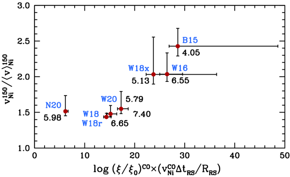
Figure 6: Dependence of the extent of ⁵⁶Ni mixing in velocity space on the hydrodynamic properties of the progenitor for models B15-2, W16-3, W18, W18r-2, W18x-2, W20, and N20-P (Table 3), whose explosions have similar energies. The uncertainties in this ⁵⁶Ni mixing are related to estimates of the velocities of the ⁵⁶Ni ejecta containing $93\%$ and $99\%$ of the total ⁵⁶Ni mass. Numbers give the helium-core masses of the corresponding progenitor models.

How strongly the fast Rayleigh-Taylor plumes that grow from the C+O core through the He layer interact with the reverse shock that develops below the He/H composition interface depends on the ratio of the time interval during which the reverse shock forms relative to the time needed by the Rayleigh-Taylor plumes originating from the (C+O)/He interface to cross the reverse shock. The greater this ratio, the weaker the interaction and the higher the terminal velocity of fast Rayleigh-Taylor plumes. The formation time of the reverse shock, $\Delta\,t_{\mathrm{RS}}$, is estimated from the hydrodynamic model as the time from when the main shock crosses the He/H composition interface to the moment at which the reverse shock forms. The characteristic time of the outward growth of Rayleigh-Taylor plumes may be measured by the ratio of the reverse shock radius at the formation epoch, $R_{\mathrm{RS}}$, to the characteristic velocity of the plumes. The latter may be identified with the maximum velocity of the bulk mass of ⁵⁶Ni at the moment just after the main shock passes the (C+O)/He composition interface, $v_{\mathrm{Ni}}^{\mathrm{CO}}$. In Table 3 we give the corresponding quantities that determine the amount of mixing of radioactive ⁵⁶Ni for models B15-2, W16-3, W18, W18r-2, W18x-2, W20, and N20-P in our simple phenomenological approach.

Figure 6 shows the extent of ⁵⁶Ni mixing in velocity space as a function of the hydrodynamic properties for our progenitor models. The extent of ⁵⁶Ni mixing is measured by the dimensionless ratio of the maximum velocity of the bulk mass of ⁵⁶Ni ejecta containing $96\%$ of the total ⁵⁶Ni mass at day 150, $v_{\mathrm{Ni}}^{\mathrm{150}}$, to the weighted mean velocity of the bulk mass of ⁵⁶Ni at the same epoch, $\langle v\rangle_{\mathrm{Ni}}^{\mathrm{150}}$, whereby we eliminate the influence of slightly different explosion energies of the models. Because the outward mixing of ⁵⁶Ni depends on the growth of Rayleigh-Taylor plumes at the (C+O)/He composition interface as well as on the interaction of those plumes with the reverse shock from the He/H composition interface, we use the product of these two physically independent measures as abscissa in Fig. 6.

Obviously, there is a correlation between the normalized extent of ⁵⁶Ni mixing and the two hydrodynamic properties that favor the mixing of radioactive ⁵⁶Ni in different progenitor models (Fig. 6). The existence of this correlation confirms the decisive role of the two selected factors on the amount of outward mixing of radioactive ⁵⁶Ni in the framework of 3D neutrino-driven simulations. In addition, the model sequence B15-2, W18x-2, W20, N20-P, W16-3, W18r-2, and W18 shows that strong radioactive ⁵⁶Ni mixing tends to be disfavored by a high helium-core mass of the progenitor model. The latter result is very important when constructing adequate progenitor models that might produce an amount of mixing of radioactive ⁵⁶Ni compatible with the spectroscopic observations of SN 1987A.

We note that this correlation becomes more obvious when we exclude model N20-P from our consideration (Fig. 6). Similarly, this model is also inconsistent with the decreasing trend of the amount of hydrogen mixed into the He shell in the model sequence B15-2, W16-3, W18x-2, N20-P, W18, W20, and W18r-2, along which the mixing of radioactive ⁵⁶Ni monotonically decreases in velocity space. Thus, the progenitor model N20 differs considerably from the other models in producing macroscopic mixing of both radioactive ⁵⁶Ni and hydrogen. It might be that the outlier status of model N20 is related to its nonevolutionary origin, as pointed out in Sect. 2.1.

We do not place much weight on model N20 for these reasons. The present set of BSG explosion models exhibits ⁵⁶Ni mixing whose strength scales roughly inversely with the helium-core mass $M_{\mathrm{He}}^{\,\mathrm{core}}$ (see the numbers next to the model names in Fig. 6). This may appear plausible because the growth factor $\log(\xi/\xi_{0})^{\mathrm{CO}}$ decreases nearly monotonically with $M_{\mathrm{He}}^{\,\mathrm{core}}$ (Table 3), which might suggest that $v_{\mathrm{Ni}}^{\mathrm{CO}}$ simply grows with higher growth factor (i.e., lower helium-core mass), thus leading to ⁵⁶Ni penetration of the hydrogen envelope with higher velocities. However, models W18 and W18r-2 do not perfectly follow this ordering in Fig. 6, and in particular, model W16-3 constitutes a clear case that contradicts such a simple causal relation: W16-3 exhibits a fairly high value of $v_{\mathrm{Ni}}^{\mathrm{CO}}$ despite its rather low value of $\log(\xi/\xi_{0})^{\mathrm{CO}}$ (see Table 3).

Nevertheless, we do not consider model W16-3 as a peculiar outlier with respect to its value of $v_{\mathrm{Ni}}^{\mathrm{CO}}$, which requires that some special physics play a role in this particular model. A detailed analysis of the explosion properties and evolution did not reveal any peculiarities in this case. Instead, we interpret the situation such that there is no clear trend of $v_{\mathrm{Ni}}^{\mathrm{CO}}$ growing with $\log(\xi/\xi_{0})^{\mathrm{CO}}$, but the results of $v_{\mathrm{Ni}}^{\mathrm{CO}}$ show basically random scatter as function of the growth factor: models W16-3, W18, and W18r-2 have very similar values of $\log(\xi/\xi_{0})^{\mathrm{CO}}$, but their $v_{\mathrm{Ni}}^{\mathrm{CO}}$ values differ considerably, whereas models N20-P, W20, W18x-2, and B15-2 possess significantly larger growth factors (more than an order of magnitude, increasing for the model sequence given) than model W16-3, but model N20-P has a lower and model W20 has a similar value of $v_{\mathrm{Ni}}^{\mathrm{CO}}$ compared to model W16-3. Therefore we conclude that the growth factor at the (C+O)/He composition interface alone cannot explain the final ⁵⁶Ni-mixing velocities. Instead, our measure of the ⁵⁶Ni mixing on the vertical axis of Fig. 6 shows a tight correlation with the product of the two factors coining the quantity on the horizontal axis of this figure. The second factor, whose physical meaning is explained above by the effects of an interaction of the ⁵⁶Ni plumes with the reverse shock from the He/H composition interface, moves model W20 with its low value of $v_{\mathrm{Ni}}^{\mathrm{150}}/\langle v\rangle_{\mathrm{Ni}}^{\mathrm{150}}$ to the left, while model W16-3 stays more toward the right, although both models have nearly the same values of $v_{\mathrm{Ni}}^{\mathrm{CO}}$.

Of course, all this reasoning is based on grounds of a fairly limited sample of 3D simulations. A simple ordering of the ⁵⁶Ni mixing with the growth factor at the (C+O)/He composition interface, $\log(\xi/\xi_{0})^{\mathrm{CO}}$, (or, equivalently, an inverse correlation with the helium-core mass) mostly contradicts models W16-3 and W20. To conclusively clarify whether both of these models are special cases requires computing a considerably larger set of BSG explosions with similar energies.

3.4 Light-curve modeling

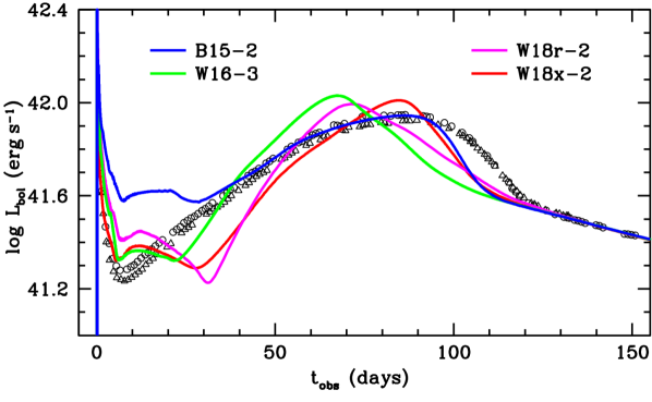
Figure 7: Bolometric light curves of models B15-2, W16-3, W18r-2, and W18x-2 compared with the observations of SN 1987A obtained by Catchpole et al. (1987, 1988) (open circles) and Hamuy et al. (1988) (open triangles).

We (Utrobin et al. 2015) have in detail performed light-curve modeling based on 3D hydrodynamic simulations of neutrino-driven explosions for the set of pre-SN models B15, W18, W20, and N20. In particular, we studied the influence of the explosion energy and the ejected ⁵⁶Ni mass on the calculated light curves. Here, we focus on the properties of the new pre-SN models W16, W18r, and W18.

Our previous hydrodynamic light-curve modeling showed that the pre-SN radii of all models considered are too large to fit the initial luminosity peak of SN 1987A. Our hydrodynamic simulations with models W16, W18r, and W18x, whose radii are smaller than those used previously (Table 1, Fig. 1b), show a much better agreement of the calculated light curves with the observed initial luminosity peak than reference model B15-2 (Fig. 7). In addition, models W16-3, W18r-2, and W18x-2 are able to synthesize amounts of radioactive ⁵⁶Ni in the general range of what guarantees a good match of the calculated light curves with the observed radioactive tail (Table 2, Fig. 7).

For SN 1987A, the total mass of radioactive ⁵⁶Ni, evaluated by equating the observed bolometric luminosity in the radioactive tail to the gamma-ray luminosity and called the observed amount of radioactive ⁵⁶Ni, is $0.0722\,M_{\sun}$ (Utrobin et al. 2015). The ⁵⁶Ni mass in the ejecta at day 150, $M^{f}_{\mathrm{Ni}}$, which matches the observed luminosity in the radioactive tail, exceeds the observed value because of the expansion-work effects (Utrobin 2007). The initial ⁵⁶Ni mass at the onset of light curve modeling, $M^{i}_{\mathrm{Ni}}$, exceeds in turn the value of $M^{f}_{\mathrm{Ni}}$ because of fallback of ⁵⁶Ni taken into account. The initial ⁵⁶Ni masses of models W16-3, W18r-2, and W18x-2 fall in between the minimum, $M_{\mathrm{Ni}}^{\,\mathrm{min}}$, and maximum, $M_{\mathrm{Ni}}^{\,\mathrm{max}}$, values (Table 2).

While the initial luminosity peak mainly depends on the pre-SN radius and the structure of the outer layers, the radioactive tail is entirely determined by the total amount of radioactive ⁵⁶Ni. The light curve in between these phases depends in addition on the explosion energy, the ejecta mass, and, in what we are interested here, the macroscopic mixing of ⁵⁶Ni and hydrogen-rich matter. A comparison of the light curves of models W16-3, W18r-2, and W18x-2 with that of model B15-2 shows that there are significant differences in the rise to the second maximum of the light curve and its dome-like look. The quality of the light-curve fits can be only partially improved by enhancing the macroscopic mixing of ⁵⁶Ni and hydrogen-rich matter. The differences in the dome-shaped part of the light curve also reflect to some extent the differences in the pre-SN structure.

Of particular interest is the question of the role of 3D macroscopic mixing in light-curve modeling of ordinary versus peculiar type IIP SN. We discuss this in Appendix A.

3.5 Comparison with observations

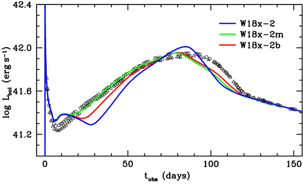
Figure 8: Bolometric light curves of model W18x-2 and two additional models W18x-2m and W18x-2b compared with the observations of SN 1987A obtained by Catchpole et al. (1987, 1988) (open circles) and Hamuy et al. (1988) (open triangles). Model W18x-2m is constructed on the basis of model W18x-2, where both ⁵⁶Ni and hydrogen are mixed artificially to match the observations as well as possible. Outward ⁵⁶Ni mixing up to 3500 km s^-1 and inward H mixing of 0.26 $M_{\sun}$ into the He core result in a good fit. Model W18x-2b is similar to model W18x-2m, but the bulk of ⁵⁶Ni is mixed up to the observed velocity of about 3000 km s^-1. The two additional models W18x-2m and W18x-2b have the unchanged initial ⁵⁶Ni mass of model W18x-2.

The light curve computed by Utrobin et al. (2015) for the reference model B15-2 fits the dome-shaped part of the observed light curve of SN 1987A during the rise to its maximum much better than those of the other previous models N20-P, W18, and W20. Model B15-2 also yields a maximum velocity of the bulk of ⁵⁶Ni that is consistent with the observed value of about 3000 km s^-1. However, a very disappointing result was that the calculated light curves of all these models, which have the SN 1987A explosion energy, disagree with the observations during the first $30-40$ days. The new models W16-3, W18r-2, and W18x-2, which have smaller pre-SN radii than those of the old models (Table 1), demonstrate a much better agreement of the calculated light curves with the observations during this early period, in particular, for the initial luminosity peak (Fig. 7).

Of the new models, W18x-2 has the most acceptable dome-shape of the light curve, in particular, with respect to the position of the main maximum. We therefore focus now on this model. A closer look reveals two essential disparities between the calculated and observed light curves for this model: a pronounced local luminosity minimum at day 27, and a too narrow, more peak-like main light-curve maximum. With the pre-SN structure being specified, these shortcomings can be improved by enhancing the macroscopic mixing. First, the more intense the macroscopic mixing of ⁵⁶Ni in velocity space, the earlier the luminosity starts to grow again to the broad dome-shaped maximum. As a consequence, the local minimum at around day 27 becomes more shallow. Second, inward mixing of hydrogen-rich matter increases the opacity and optical depth of the inner ejecta, which in turn give rises to a wider and less luminous dome-shaped light-curve maximum.

The resulting effect of enhanced artificial macroscopic mixing is illustrated by the additional model W18x-2m in Fig. 8. Imposing an outward mixing of ⁵⁶Ni up to 3500 km s^-1 and an inward mixing of 0.26 $M_{\sun}$ of hydrogen into the helium core in the hydrodynamic light-curve modeling, we obtain a better agreement with the observations of SN 1987A than for model W18x-2. The agreement is only partial, and two shortcomings related to the pre-SN properties still remain. The small bump in the computed luminosity at day 10 is caused by the inadequate density distribution in the outer layers. Reducing the relatively strong ⁵⁶Ni mixing up to a velocity of 3500 km s^-1 in model W18x-2m to the observational constraint of about 3000 km s^-1 in the additional model W18x-2b causes the bump to become more prominent and emphasizes the shortcoming of the pre-SN structure. The luminosity deficit during the transition from the broad maximum to the radioactive tail can be mitigated by an increase in ejecta mass and a proportional increase in explosion energy (Utrobin et al. 2015).

In the sequence of models W18r-2, W20, W18, N20-P, W18x-2, W16-3, and B15-2, with comparable and SN 1987A-like explosion energies and a growing amount of mixing of radioactive ⁵⁶Ni in velocity space (Table 2, Fig. 6), only model B15-2 yields the maximum velocity of the bulk mass of ⁵⁶Ni of 3370 km s^-1 consistent with the spectral observations of SN 1987A, while all other models fall short of the required mixing. However, model B15, with the lowest helium-core mass of 4.05 $M_{\sun}$ of the available pre-SN models and the right amount of ⁵⁶Ni mixing, is inconsistent with the observational data of Sanduleak $-69^{\circ}202$, which suggest a single star with a helium-core mass of about 6 $M_{\sun}$.

The analysis of the line profiles in the nebular phase (Chugai 1991; Kozma & Fransson 1998; Maguire et al. 2012) and the 3D view of molecular hydrogen in SN 1987A (Larsson et al. 2019) showed that hydrogen is mixed into the core to velocities $\leq$700 km s^-1. Hydrodynamic models based on 3D neutrino-driven simulations with SN 1987A-like explosion energies demonstrate that hydrogen in the innermost layers of the ejecta expands with velocities lower than 100 km s^-1, in good agreement with the observations. In addition, Kozma & Fransson (1998) constrained the mass of hydrogen-rich gas mixed within 2000 km s^-1 to about 2.2 $M_{\sun}$. Our favorite models B15-2 and W18x-2 yield hydrogen matter mixed within 2000 km s^-1 of 0.922 $M_{\sun}$ and 0.847 $M_{\sun}$, respectively (Table 2), which is in qualitative agreement with the observational constraint.

4 Conclusions

Performing 3D neutrino-driven explosion simulations and subsequent light curve modeling, we compared the results with the observations of SN 1987A and draw the following main conclusions:

• Hydrodynamic light-curve modeling for a set of previously used pre-SN models (B15, W18, W20, and N20) showed that the pre-SN radii of all these models are too large to fit the initial luminosity peak of SN 1987A. In addition, the structure of the outer layers of these models cannot reproduce the observed light curve during the first 30–40 days (Utrobin et al. 2015). Hydrodynamic simulations with new progenitor models (W16, W18r, and W18x) that have smaller radii than the other models demonstrate a much better agreement of the calculated light curves with the observed one in the initial luminosity peak and during the first 20 days than our old hydrodynamic models.

• The initial (at the onset of light-curve modeling) ⁵⁶Ni masses required to match the observations of the radioactive tail of SN 1987A fall in between the minimum and maximum estimates obtained in our 3D explosion models, implying that all 3D neutrino-driven simulations under study are able to synthesize the ejected amount of radioactive ⁵⁶Ni for explosion energies in the general range of what is needed to explain the observed light curve.

• A sequence of models (B15-2, W18x-2, W20, N20-P, W16-3, W18r-2, and W18) with nearly the same explosion energies showed that the extent of outward radioactive ⁵⁶Ni mixing in the framework of the 3D neutrino-driven simulations depends mainly on the following two hydrodynamic properties of the progenitor model: A high growth factor of Rayleigh-Taylor instabilities at the (C+O)/He composition interface, and a weak interaction of fast Rayleigh-Taylor plumes, with the reverse shock occurring below the He/H composition interface, seem to be a sufficient condition for efficient outward mixing of ⁵⁶Ni into the hydrogen envelope.

• The analysis of SN 1987A observations revealed the fact that radioactive ⁵⁶Ni was mixed in the ejecta up to a velocity of about 3000 km s^-1. In our 3D neutrino-driven simulations, only model B15-2 yields a maximum velocity of the bulk of ⁵⁶Ni consistent with the observations, and only this model is therefore able to reproduce the increase to the light-curve maximum of SN 1987A with good agreement. However, the helium-core mass of $4.05\,M_{\sun}$ of the pre-SN model B15 is inconsistent, assuming single-star evolution, with the observational data of the BSG Sanduleak $-69^{\circ}202$ star, which suggest a star that has a helium-core mass of $\approx$6 $M_{\sun}$ at the time of its explosion.

From the 3D simulations we presented for macroscopic mixing that occurs during neutrino-driven explosions, we conclude that existing evolutionary models of single stars cannot simultaneously fulfill the observational requirements of the location of the BSG Sanduleak $-69^{\circ}202$ star in the Hertzsprung-Russell diagram and the observed amount and extent of outward mixing of radioactive ⁵⁶Ni. Two speculative possibilities for a solution of this problem have been proposed: a progenitor with a more rapidly rotating iron core and a jet-induced explosion (Khokhlov et al. 1999; Wheeler et al. 2002; Wang et al. 2002), or a binary evolution scenario (Hillebrandt & Meyer 1989; Podsiadlowski & Joss 1989; Podsiadlowski et al. 1990, 1992). While the question of rapid rotation of the iron core remains open, the formation of the SN 1987A triple-ring system was explained by Podsiadlowski et al. (2007) and Morris & Podsiadlowski (2009) in the scenario of a binary merger model.

In our study the rotating progenitor models W16, W18, W18r, and W18x have moderate angular momenta on the main sequence of $(2.7,3.1,3.1,\mathrm{and}\ 2.3)\times 10^{52}$ erg s, respectively (Sect. 2.1). To estimate an initial rotation rate of the resultant pulsar, we assumed that the inner 1.7 $M_{\sun}$ core collapses to a newly born neutron star with a gravitational mass of 1.4 $M_{\sun}$ and a radius of 12 km, and that angular momentum is conserved during the collapse. For models W16, W18, W18r, and W18x, the estimates for the spin periods (or, to be more accurate, their lower limits) are 10.6, 10.3, 12.5, and 10.0 ms, respectively. The transport of angular momentum by magnetic fields during the collapse might have increased the period, but we note that even this maximum value would imply a small contribution from rotation to the explosion energy. We ignored such a progenitor rotation because it is so slow that it does not affect the neutrino-driven mechanism, nor is it an efficient energy source for a magnetohydrodynamics mechanism. This is consistent with the lack of any bright pulsar in the current remnant (Alp et al. 2018), which supports slow rotation of the degenerate stellar core. Therefore a scenario involving the formation of (jittering) jets (Soker 2017; Bear & Soker 2018) seems disfavored as well.

However, slow core rotation does not preclude that rotation, for instance, from a binary progenitor scenario, contributes to mixing and asymmetry in the pre-collapse star and in the explosion. Menon & Heger (2017) presented the results of a stellar evolution study of binary merger models for the progenitor of SN 1987A. Their Hertzsprung-Russell diagram shows that binary merger models with a primary star of 16 $M_{\sun}$ and secondaries ranging from 2 to 8 $M_{\sun}$ evolve to compact pre-SN models in or close to the region of the observed properties of Sanduleak $-69^{\circ}202$. The helium-core masses of all of these pre-SN models are lower than 4 $M_{\sun}$, which seems promising for producing the high-velocity ⁵⁶Ni-rich ejecta observed in the spectra of SN 1987A. Recently, Menon et al. (2019) have made the first successful step on the road of applying these binary merger progenitors to hydrodynamically modeling the light curve of SN 1987A, which was computed with an artificial “boxcar” mixing of the chemical species and an explosion by a piston in spherically symmetric geometry. The appropriate 3D simulations of neutrino-driven explosions of these SN 1987A progenitor models are in progress to determine the corresponding mixing self-consistency.

We conclude that the lack of an adequate progenitor model for the well-observed and well-studied SN 1987A remains a challenge for the theory of stellar evolution of massive stars.

Appendix A Role of 3D macroscopic mixing in light-curve modeling of ordinary and peculiar type IIP supernovae

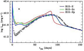
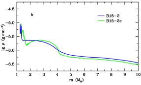
Figure 9: Effect of 3D macroscopic mixing on the bolometric light curve (a) and the density profile as a function of interior mass at the mapping moment of $t=61,213$ s (b). The reference model B15-2 (blue) is compared with model B15-2c (green), which is the 1D analog of model B15-2. Model B15-2c is based on the pre-SN model B15, is exploded by a piston, and its chemical composition is identical to that of the averaged 3D model B15-2. For a comparison, the red line shows the bolometric light curve of model B15-2p, which is based on the unmixed pre-SN model B15 and exploded by a piston. Open circles (Catchpole et al. 1987, 1988) and open triangles (Hamuy et al. 1988) are the bolometric data of SN 1987A.

The first attempts to hydrodynamically model the peculiar type IIP SN 1987A faced an unexpected problem: the original, unmixed evolutionary pre-SN models produced a half-truncated maximum of the light curve like that of model B15-2p in Fig. 9a (cf. Woosley 1988; Arnett & Fu 1989). This result is inconsistent with the observations of SN 1987A. A similar problem arose in modeling ordinary type IIP SNe with evolutionary pre-SN models when theoretical light curves exhibited a conspicuous shoulder-like (Woosley & Heger 2007; Morozova et al. 2015; Sukhbold et al. 2016) or spike-like (Chieffi et al. 2003; Young 2004) feature during the decline in luminosity from the plateau to the radioactive tail, which is not seen in observations. For both peculiar and ordinary type IIP SNe, artificial mixing of the chemical species was invoked to solve these problems.

The study of the ordinary type IIP SN 1999em showed that turbulent mixing induced by 3D neutrino-driven explosions causes both flattening of the density distribution at the location of the He/H interface and macroscopic mixing of chemical species, which in turn cause the monotonic decline in luminosity from the plateau to the radioactive tail as it is observed (Utrobin et al. 2017). In our previous paper on the peculiar type IIP SN 1987A (Utrobin et al. 2015), we focused mainly on macroscopic mixing of radioactive ⁵⁶Ni and hydrogen that occur during the explosion. Here we revisit the issue of turbulent mixing in SN 1987A in the context of modifying the density distribution compared to 1D hydrodynamic models.

To clarify the influence of mixing on the density distribution and the light curve for the explosion of a BSG star, we compared our reference model B15-2 (Table 2) with its 1D analog B15-2c. The latter is based on the pre-SN model B15 (Table 1), is a piston-driven explosion, and its chemical composition is identical to that of the averaged 3D model B15-2 (Fig. 5a). Model B15-2c thus constructed permits us to refine the effect of turbulent mixing on the density distribution at the location of the He/H composition interface from other effects.

Figure 9b shows that a density step (contact discontinuity) at the outer edge of the helium core (at about 4 $M_{\sun}$) appears after the SN shock crossed the He/H composition interface in 1D model B15-2c, while the averaged density distribution of the 3D model B15-2 is smooth and has no signature of a density step at the location of the He/H interface, similar to the 3D explosion of a RSG star (Utrobin et al. 2017). The smoothness of the density distribution reflects a characteristic feature of our 3D neutrino-driven explosion simulations: large-scale turbulent mixing occurs, which smoothes the density distribution. The less prominent density step in the case of model B15-2c compared to that of model L15-pn (Utrobin et al. 2017, see Fig. 8a) is related to a weaker density contrast at the outer edge of the helium core in the BSG model B15 (Fig. 1c) compared to that of the RSG model L15 (Utrobin et al. 2017, see Fig. 2a).

The density structure within the helium core of the 1D hydrodynamic model B15-2c does not affect the shape of the light curve, which is similar to that of the reference model B15-2 (Fig. 9a). The slightly higher luminosity of model B15-2c compared to that of model B15-2 during the first 20 days is caused by the difference in density outside the helium core (Fig. 9b). The lower density in model B15-2c means that the star is more extended (a given mass is distributed in a larger volume), leading to larger radiation losses. This situation raises the question why the 1D density structure for the peculiar type IIP SN 1987A does not exhibit any conspicuous spike-like feature that is not observed, whereas it does in the 1D hydrodynamic model for the ordinary type IIP SN 1999em (Utrobin et al. 2017). There are two reasons behind this behavior. First, the step-like feature in density at the He/H interface in model B15-2c is less prominent than that of model L15-pn, as pointed out above. Second, the photosphere crosses the sharp He/H interface in model B15-2c at around day 85 (Fig. 9a) and in model L15-pn at around day 135 (Utrobin et al. 2017, see Fig. 7), when the sources of the internal energy in these models are quite different.

At around day 85, the luminosity of the peculiar type IIP SN 1987A is completely powered by gamma-rays from radioactive ⁵⁶Co, while the internal energy deposited by the shock wave has already been exhausted by about day 30. The difference in density between models B15-2c and B15-2 in the mass range from 2 to 4 $M_{\sun}$ (Fig. 9b) does not cause an essential energy excess deposited by gamma-rays from radioactive ⁵⁶Co in model B15-2c compared to model B15-2, and as a consequence, results in a close similarity between the corresponding light curves near maximum (Fig. 9a). At the same time, a comparison of model B15-2p based on the unmixed pre-SN model B15 with model B15-2c, which has a chemical composition identical to that of the averaged 3D model B15-2, shows that mixing induced by the 3D neutrino-driven explosion eliminates the unobserved half-truncated maximum of the light curve of model B15-2p (Fig. 9a). Thus, turbulent mixing that occurs during the 3D neutrino-driven explosion of a BSG star causes both smoothing of the density distribution and macroscopic mixing of the chemical species, but only the latter affects the light curve.

In contrast to SN 1987A, the release of the internal energy deposited during the propagation of the shock wave through the pre-SN envelope produces the luminosity of the ordinary type IIP SN 1999em not only during the plateau phase, but also during the monotonic decline in luminosity from the plateau to the radioactive tail. In turn, the release of the internal energy deposited by radioactive decays becomes essential just before entering the radioactive tail. At around day 135 in model L15-pn for SN 1999em, when a pronounced spike appears in the luminosity decline from the plateau to the radioactive tail, the internal energy deposited by the shock remains dominant in powering the luminosity. Utrobin et al. (2017) showed that both the density step at the outer edge of the helium core and the unmixed chemical composition of the evolutionary pre-SN model are responsible for the unobserved spike in the light curve that is computed with hydrodynamic models that are exploded by a piston in spherically symmetric geometry, and that this spike disappears only in the framework of the 3D neutrino-driven explosion simulations.