PREDICTING “DESIGN GAPS" IN THE MARKET: DEEP CONSUMER CHOICE MODELS UNDER PROBABILISTIC DESIGN CONSTRAINTS

Abstract

Predicting future successful designs and corresponding market opportunity is a fundamental goal of product design firms. There is accordingly a long history of quantitative approaches that aim to capture diverse consumer preferences, and then translate those preferences to corresponding “design gaps” in the market. We extend this work by developing a deep learning approach to predict design gaps in the market. These design gaps represent clusters of designs that do not yet exist, but are predicted to be both (1) highly preferred by consumers, and (2) feasible to build under engineering and manufacturing constraints. This approach is tested on the entire U.S. automotive market using of millions of real purchase data. We retroactively predict design gaps in the market, and compare predicted design gaps with actual known successful designs. Our preliminary results give evidence it may be possible to predict design gaps, suggesting this approach has promise for early identification of market opportunity.

1 Introduction

Predicting consumer preferences for future design concepts is a fundamental task for product design enterprises [21]. For example, consumer preferences drove “crossover vehicles” to overtake the previously dominant SUV segment within just years of introduction to the U.S. automotive market [20].

To predict consumer preferences, quantitative models of human choice have been researched and developed for more than a century [44, 47]. In general, these methods estimate a predictive model of future consumer preferences using stated or revealed data from past consumer choices over design alternatives. These predictive models can then be used to improve design or managerial decisions such as predicting consumer demand [39] or market segmentation [53]. The success of these methods is underscored by their adoption by product design enterprises–one of the most popular methods, conjoint analysis, has over 18,000 applications a year [33].

One of the most challenging consumer preference prediction tasks is to identify “design gaps" in the market. These design gaps are clusters of designs that do not yet exist, are perhaps unknown to the firm, yet represent potentially significant market opportunity. Early identification of design gaps offers firms competitive advantage due to first mover effects.

The challenge in predicting design gaps is due to the number of statistical unknowns. One can conceptually group consumer preference prediction tasks by their unknowns into three categories of increasing difficulty: The first category, with the least unknowns, is to predict what unknown consumers would prefer among known and existing product designs; e.g., product recommendation by online retailers. The second category is to predict what unknown consumers would prefer among known and not existing product designs; e.g., SUV concept designs during prototyping. The third category predicts what unknown consumers would prefer among unknown and not existing product designs.

In this work, we address this third category. This aims at the question: Can firms quantitatively predict design gaps that represent potential market opportunities at the earliest stages? With new product development, could automotive manufacturers have predicted years in advance that the crossover vehicle segment represented a massive market opportunity? With updating existing products, could the same manufacturers identify new combinations of infotainment features and marketing cues that appeal to millenials?

We introduce a deep learning approach that aims to identify design gaps hidden in large-scale data. This approach predicts regions of the design space that (1) have high predicted consumer preference, and (2) are feasible to build according to probabilistic estimates of design constraints from engineering, manufacturing, and other downstream design processes. This approach combines and builds on research from quantitative marketing in consumer choice modeling, and engineering design for bounding design feasibility within the design space.

We test this approach on several years of millions of actual purchase data from the U.S. automotive market. To artificially induce "design gaps," we use actual purchase data to retroactively construct unknown consumers and unknown and not existing product designs. Validity is then assessed by how well the proposed deep learning approach predicts design space regions containing held-out new design entrants to the market.

Our preliminary results give evidence that this approach may lead to design gaps. This offers the following contributions:

1. Deep heterogeneous consumer choice models can significantly improve held-out choice prediction accuracy.

2. Deep unsupervised models can efficiently estimate probabilistic design constraints to bound the design space.

3. Given (1) and (2), prediction of design gaps may be possible using information-theoretic disaggregate choice metrics.

This approach does not predict the actual design itself, nor does it directly predict market opportunity. It instead aims to highlight significantly reduced promising subsets of the feasible design space rather than the otherwise exponential number of possible designs. In other words, this approach still requires designers and market researchers investigate proposed design gaps, offering instead a scalable data-driven approach to augment both strategic marketing and the creative design process.

The rest of this paper is structured as follows: Section 2 discusses related work in marketing and design. Section 3 formulates a consumer choince model under design constraints. Section 4 conducts an experiment using real purchase data. Section 5 discusses implications and opportunities for future work. Section 6 offers conclusions.

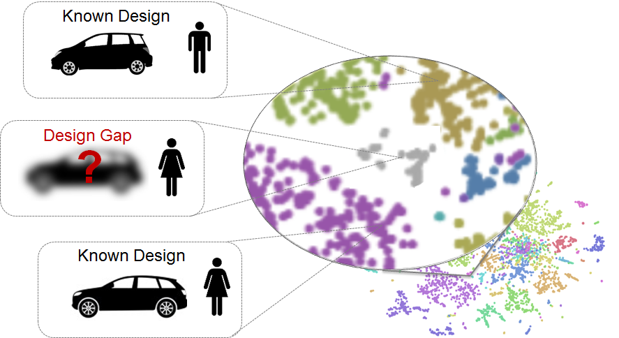
Figure 1: High-level goal of this work, predicting potentially unknown “design gaps” in the market.

2 Related Work

We describe related work primarily in two communities, quantitative marketing and engineering design. Our work builds on conventions in each of these communities.

2.1 Consumer Preference Modeling

There is long and rich history of modeling techniques aimed at capturing consumer preference and choice decisions over a set of alternatives, across fields such as psychology, economics, marketing, and product design.

Most relevant to our work is the research carried out in capturing consumer choice in a probabilistic model used to inform design decisions. One of the most popular models is this group is conjoint analysis, in which consumers have a “part-worth vector” describing their affinity for design attributes (e.g., color, price, horsepower) through a linear relationship. These models have their roots in psychology [44, 48, 26] and economics [51], but received major attention for improving design and marketing during the supermarket scanner data revolution [40].

Since this first data revolution, several extension to capture the diversity of consumer preferences, referred to as consumer heterogeneity, have received considerable attention. An early yet still widely used model of heterogeneity extends the basic conjoint formulation to having a hierarchical prior distribution [39]. This prior encodes the idea that the population is centered around an average consumer, and that heterogeneity is related to the distance from the average. In general, the notion of modeling consumer heterogeneity improves tasks such as consumer demand or market segmentation [53].

Within design research, consumer choice models are found widely in decision-based formulations of design [14, 52, 23]. Recently several works have focused on modeling heterogeneous consumer consideration for designs [30], building off again original findings in psychology [36]. These formulations note that preference decisions are not made randomly over set of existing designs, but rather a subset where attributes are traded off [13].

Another key concept adopted by our work is the idea of higher-level abstractions of the preference task. For example, consumers do not necessarily purchase a vehicle for its number of valves per cylinder, but rather meaningful attributes such as perceived luxuriousness and external image. This notion has been observed in many guises across design [32, 31], psychology [5], and marketing [49].

Our work aims to estimate both consumer heterogeneity and higher-level preference abstractions as “features” discovered from the data [7]. We place flexible mathematical assumptions on the form of consumer heterogeneity, instead letting it be “learned” by recent advances in deep learning over large data sets. Our work is similar in this guise to machine learning work in marketing [45] for efficient consumer choice estimation algorithms, as well as flexible function forms on preference itself [9, 24]. In addition, we use the well-known concept of “borrowing strength” of Bayesian conjoint analysis models [22], albeit with a deep neural network formulation.

2.2 Design Constraint Modeling

The aim of modeling design feasibility is to capture constraints on new potential design concepts, physical or perhaps implicit from some other source. For example, the design may have engineering constraints due to physical relations between aerodynamics and vehicle handling dynamics, physical manufacturing constraints based on scalability of existing powertrain or chassis platforms, and perceptual constraints such as brand recognition and perceived image cues [6].

These constraints are important when identifying design gaps. Specifically, one should take reservation when optimizing consumer preferences with respect to an unbounded space of designs. Such an optimization can lead to the so-called “million-dollar car," which theoretically has high consumer demand but is unrealistic due to violations of engineering and fiscal constraints.

Several major pathways towards design representations that encode realistic constraints have been developed by the design community. Direct analytic modeling uses deterministic mathematical relationships amongst variables. Conceptually related to our work is [27], who combine consumer choice models and analytic design models. Recent work includes mixing sophisticated consumer choice consideration models with analytic design models [25]. Simulation-based approaches to design feasibility are widely-used, for example, [3], who develop an explicit generative model of all hybrid vehicle powertrain architectures. Their model has conceptual similarities with our design gap identification approach, as both perform rejection sampling. Rule-based design representations use smaller elements and rules on design synthesis. For example, [43] and [37] use shape grammars with aesthetic rules for a parametrized vase designs.

Most related to our work is that of using probabilistic models of design representations. As noted in [50], large-scale data is enabling better capture of consumer choice preferences for early-stage design. [46] collect large-scale social media data for mining consumer preferences. Similar to our work is [34], who use restricted Boltzmann machines to model consumer choices. Likewise, in marketing, [15] use the same restricted Boltzmann machine for predicting market baskets, and note its relationship with multinomial logit models. Our work is similar in that we use a multinomial logit model with a “deep” architecture for both learning consumer preferences, as well as capturing design constraints. As a result, our approach is a combination of both discriminatative and generative models [28, 41, 34].

3 Problem Formulation

The high-level goal of the following mathematical formulation is to capture the relationship between consumers and product designs that are realistically feasible. In particular, we are interested in an accurate relationship between not just consumers and designs that currently exist, but between consumers and designs that are theoretically possible. This level of generalization accuracy requires not just capturing the relationship between consumers and designs, but capturing the relationship between existing designs and future designs as well as existing consumers and future consumers.

Let us denote consumers $\mathbf{x}_{c}\in\mathcal{X}_{c}\subseteq\mathbb{R}^{M_{c}}$ and designs $\mathbf{x}_{d}\in\mathcal{X}_{d}\subseteq\mathbb{R}^{M_{d}}$ using vectors, and denote the $c^{th}$ customer as $\mathbf{x}_{c}^{(c)}$ and the $d^{th}$ existing design as $\mathbf{x}_{d}^{(d)}$. The consumer space $\mathcal{X}_{c}$ and design space $\mathcal{X}_{d}$ are both bounded subsets of the real values. We also assume that there is a finite set of existing design alternatives for consumers to choose from $\{\mathbf{x}_{d}^{(d)}\}_{d=1}^{D}$, in which the true purchased or preferred design is denoted as an indicator vector $\mathbf{y}\in\{0,1\}^{D}$ over all existing designs, as well as the shorthand $y^{(d)}\in\{0,1\}$ as the $d^{th}$ element of the indicator vector $\mathbf{y}$.

Quantitative choice models assume a parametric utility function $U(\mathbf{x}_{c},\mathbf{x}_{d},\theta):\mathcal{X}_{c}\times\mathcal{X}_{d}\rightarrow\mathbb{R}$, where $\theta$ are parameters of the utility model that index consumer and design pairs to a real number value in which higher numbers correspond to higher preference [51]. This utility function lies within a probabilistic choice or preference model, in which the choice model maps the consumer response task (e.g., ranking, rating, choice) to values of utility [26]. In doing so, the choice model accounts for uncertainty from factors such as missing latent variables, model mispecification, and measurement error [39].

We aim to predict how much the $c^{th}$ consumer $\mathbf{x}_{c}^{(c)}$ prefers the $d^{th}$ product design $\mathbf{x}_{d}^{(d)}$ among the entire set of $D$ designs. This invokes representing the $c^{th}$ consumer’s utility function for the $d^{th}$ design in relation to all other designs $i=1\ldots D$.

$$p(y^{(d)}=1|\mathbf{x}_{c},\mathbf{x}_{d})$$ (1)

$$=p\left(U\left(\mathbf{x}_{c}^{(c)},\mathbf{x}_{d}^{(d)}\right)+\epsilon^{(c,d)}>\left\{U\left(\mathbf{x}_{c}^{(c)},\mathbf{x}_{d}^{(i)}\right)+\epsilon^{(c,i)}\right\}_{i=1}^{D}\right)$$

where $\epsilon^{(c,d)}$ is extreme value distributed [11], resulting in a softmax function for choice probability [26].

The full Bayesian joint likelihood $\mathcal{L}_{A}(\theta;\mathbf{y},\mathbf{x}_{c},\mathbf{x}_{d})$ of $p$ over $\mathcal{X}_{c}\times\mathcal{X}_{d}\times\mathcal{Y}$ acts as a generative distribution of consumer preference under design constraints that bound $\mathcal{X}_{d}$ and consumer heterogeneity that bound $\mathcal{X}_{c}$. We take a fully Bayesian approach, in that we invoke prior distributions over consumers $p(\mathbf{x}_{d})$ and design $p(\mathbf{x}_{d})$.

$$\mathcal{L}_{A}(\theta;\mathbf{y},\mathbf{x}_{c},\mathbf{x}_{d}) = p(\mathbf{y}|\mathbf{x}_{c},\mathbf{x}_{d})p(\mathbf{x}_{d})p(\mathbf{x}_{c})$$

$$p(\mathbf{y}|\mathbf{x}_{c},\mathbf{x}_{d}) = \mathrm{M}(\mathbf{y})$$

$$p(\mathbf{x}_{d}) = \mathcal{N}\left(\mathbf{x}_{dr};\boldsymbol{\mu},\Sigma_{d}\right)\prod_{b}\mathrm{B}(x_{db,b})\prod_{m}\mathrm{M}(\mathbf{x}_{dm,j})$$ (2)

$$p(\mathbf{x}_{c}) = \frac{1}{N}\sum_{i}\delta(\mathbf{x}_{c}-\mathbf{x}_{c}^{(i)})$$

where $\mathcal{N}\left(\cdot\right)$ is the multivariate Gaussian density with mean vector $\boldsymbol{\mu}$ and covariance matrix $\Sigma_{d}$, $\mathrm{B}(\cdot)$ is the Bernoulli density with the sigmoid function $p(x_{db,b}=1)=\frac{e^{\theta_{b}x_{d}}}{1+e^{\theta_{b}x_{d}}}$ , $\mathrm{M}(\cdot)$ is the multinomial density using the softmax function $p(\mathbf{y}|\mathbf{x}_{c},\mathbf{x}_{d})=\frac{e^{U\left(\mathbf{x}_{c},\mathbf{x}_{d}^{(d)}\right)}}{\sum_{i}e^{U\left(\mathbf{x}_{c},\mathbf{x}_{d}^{(i)}\right)}}$ for consumer choice preferences or $p(\mathbf{x}_{d,m}=k)=\frac{e^{\theta_{m}^{(k)}\mathbf{x}_{d}}}{\sum_{i}e^{\theta_{m}^{(i)}\mathbf{x}_{d}}}$ for categorical design variables, and $\delta(\cdot)$ is a Dirac delta function used to represent the empirical distribution of consumers.

3.1 Feature Learning

The consumer choice prediction model given in Equation (1) has been widely used across disciplines such as psychology, marketing, economics, and design. While the underlying mathematical formulation is conceptually the same, common modeling challenges are often addressed in separate manners according to the conventions of the field. This offers us the opportunity to build on modeling assumptions across fields, making explicit our modeling goals in an effort to improve predictive model fidelity.

3.1.1 Consumer Heterogeneity and Design Feasibility

One of the major challenges in the choice modeling research is how to represent consumer preference heterogeneity; in short, the diversity in human preferences. Mathematical representations to encode heterogeneity involve assuming a distribution over customer variables as they relate to the design. Implicitly, this distribution encodes constraints on the space of consumers $\mathcal{X}_{c}$; for example, certain hobbies may be constrained by income and leisure time.

Quantitative marketing methods often explicitly encode consumer constraints, such as monotonic relationships on price sensitivity [33]. Ever more sophisticated constraint mechanisms often integrate research marketing and psychology research findings, such as partitioning the set of existing designs $\{\mathbf{x}_{d}^{(d)}\}_{d=1}^{D}$ into a much smaller consideration set [13, 36, 30], or violations of rationality assumptions [16].

At the same time, one of the major challenges in engineering design is the formulation of design representations that are flexible, yet physically accurate. As described in Section 2, design representations include several formulations. Common to all of them is the desire to encode constraints for the space of designs $\mathcal{X}_{d}$, in which the diversity of possible designs is captured.

This analogy between constraints on the diversity of consumer heterogeneity and the diversity of design constraints allows us to take a similar probabilistic approach between these two spaces. Our approach uses large-scale data to learn the set of constraints that bound both consumers and designs.

3.1.2 Feature Representation

To estimate the diverse constraints in both the consumer space and design space, we build on substantial research that consumers consider “attributes” or “features” of the design (e.g., ‘perceived luxuriousness’) rather than the original variables (e.g., ‘valves per cylinder’). We aim to learn consumer features $\mathbf{h}_{c}\in\mathcal{H}\in\mathbb{R}^{K}$ and design features $\mathbf{h}_{d}\in\mathcal{H}\in\mathbb{R}^{K}$ that efficiently represent and constraint the information about the consumer variables $\mathbf{x}_{c}$ and design variables $\mathbf{x}_{d}$ at a more abstract level closer to the consumer’s actual preference task.

Furthermore, we aim to impose “useful" probabilistic structure for this new feature representation of the design space $p(\mathbf{h}_{d}|\mathbf{x}_{d})p(\mathbf{x}_{d})$, while keeping $\mathbf{h}_{d}$ maximally informative about the consumer preference choice $\mathbf{y}$. This structure is important for design gap prediction as it allows us a manageable representation of the otherwise high-dimensional, highly-nonlinear, and discontinuous structure of the original variables $\mathbf{x}_{d}$ of the design space (e.g., interpolations between $\frac{1}{2}$-ton trucks and turbocharged convertibles). Specifically, learning a “smoother” space allows reasonable and efficient sampling and optimization, while dimensionality reduction helps ameliorate the otherwise exponential number of possible concept design.

Accordingly, the original choice model given in Equation (1) is now updated with a new utility formulation $U(\mathbf{h}_{c},\mathbf{h}_{d},\theta):\mathcal{H}^{2}\rightarrow\mathbb{R}$ as follows.

$$p\left(U\left(\mathbf{h}_{c}^{(c)},\mathbf{h}_{d}^{(d)}\right)+\epsilon^{(c,d)}>\left\{U\left(\mathbf{h}_{c}^{(c)},\mathbf{h}_{d}^{(i)}\right)+\epsilon^{(c,i)}\right\}_{i=1}^{D}\right)$$ (3)

We assume conditional independencies between preference responses and the original variables given on their feature representations. This assumption ensures customer and design features contain the maximal possible information for the consumer preference prediction task. Our equivalent learning objective is now to predict how much the $c^{th}$ consumer $\mathbf{h}_{c}^{(c)}$ prefers the $d^{th}$ product design $\mathbf{h}_{d}^{(d)}$ among the entire set of $D$ designs. This updates Equations (1) and (2) by representing the $c^{th}$ consumer’s utility function for the $d^{th}$ design in relation to all other designs $i=1\ldots D$.

The full Bayesian joint probability distribution $p$ over $\mathcal{X}_{c}\times\mathcal{X}_{d}\times\mathcal{Y}$ is now,

$$\mathcal{L}_{A}(\theta;\mathbf{y},\mathbf{x}_{c},\mathbf{x}_{d}) =p(\mathbf{y}|\mathbf{x}_{c},\mathbf{x}_{d})p(\mathbf{x}_{d})p(\mathbf{x}_{c})$$

$$=p(\mathbf{y}|\mathbf{h}_{c},\mathbf{h}_{d})p(\mathbf{h}_{c}|\mathbf{x}_{c})p(\mathbf{h}_{d}|\mathbf{x}_{d})p(\mathbf{x}_{d})p(\mathbf{x}_{c})$$

Learning these feature representations is challenging due to both the heterogeneous variable types of the data (i.e., real, binary, categorical), as well as the desire to encode “useful” probabilistic structure in the data. Note that the inner product between consumers $\mathbf{h}_{c}$ and designs $\mathbf{h}_{d}$ ensure that consumer and design information interacts (i.e., we are not just performing classification). In practice, we estimate $p(\mathbf{y}|\mathbf{h}_{c}\mathbf{h}_{d})=\mathrm{M}(\mathbf{y}|\mathbf{h}_{c}^{T}\mathbf{H}_{d})$ , where $\mathbf{H}_{d}$ is a $K\times D$ matrix of all existing designs.

3.2 Deep Choice Model under Design Constraints

To impose the “useful" probabilistic structure required to efficiently traverse the feature representation of the design space $p(\mathbf{h}_{d}|\mathbf{x}_{d})p(\mathbf{x}_{d})$, we now introduce modeling assumptions that aim to impose structure while being amenable to recent advances in deep learning.

To this end, we adopt an approach recently popularized in deep learning called black-box variational inference. This approach aims to approximate complex probability distributions by variationally bounding the complex distribution with a more manageable joint distribution with introduced latent random variables [4]. In particular, we build on variational autoencoders as introduced in [19].

Our approach makes two minor extensions. First, given that we are working in a supervised learning regime (i.e., we eventually predict consumer preferences over new concept designs to discover “design gaps”), we include an extension that introduces an information signal to the design feature representation from the preference task. This extension is conceptually similar to semi-supervised approaches with a known labels for the encoded design representation, but different in that our supervision occurs after interaction with the consumer space [18, 42]. Second, given the heterogeneity of variable types for our data (i.e., real, binary, and categorical), we include exponential family derivations of the corresponding likelihoods in the original design variable space.

Taking the original likelihood function $\mathcal{L}_{A}(\theta,\phi;\mathbf{y},\mathbf{x}_{c},\mathbf{x}_{d})$, we introduce a approximation density $q(\mathbf{h}_{d}|\mathbf{x}_{d})$, which we will use to invoke desired “useful” probabilistic structure for the design feature representation $\mathbf{h}_{d}$.

$$\mathcal{L}_{A}(\theta,\phi;\mathbf{y},\mathbf{x}_{c},\mathbf{x}_{d}) =\int_{\mathbf{h}_{d}}\log[p(\mathbf{y},\mathbf{x}_{c},\mathbf{x}_{d})]q(\mathbf{h}_{d}|\mathbf{x}_{d})d\mathbf{h}_{d}$$

$$=\int_{\mathbf{h}_{d}}q(\mathbf{h}_{d}|\mathbf{x}_{d})[\log\frac{p(\mathbf{y},\mathbf{x}_{c},\mathbf{h}_{d},\mathbf{x}_{d})}{q(\mathbf{h}_{d}|\mathbf{x}_{d})}$$

$$+\log\frac{q(\mathbf{h}_{d}|\mathbf{x}_{d})}{p(\mathbf{h}_{d}|\mathbf{y},\mathbf{x}_{d})}]d\mathbf{h}_{d}$$

$$=\mathbb{E}_{q(\mathbf{h}_{d}|\mathbf{x}_{d})}\left[\log\frac{p(\mathbf{y},\mathbf{x}_{c},\mathbf{h}_{d},\mathbf{x}_{d})}{q(\mathbf{h}_{d}|\mathbf{x}_{d})}\right]$$

$$+\mathcal{D}_{KL}\left[q(\mathbf{h}_{d}|\mathbf{x}_{d})||p(\mathbf{h}_{d}|\mathbf{y},\mathbf{x}_{d})\right]$$

The non-negativity of the Kullback-Leibler divergence $\mathcal{D}_{KL}\left[\cdot\right]$ allows us to only focus on the first term $\mathcal{L}_{B}(\theta,\phi;\mathbf{y},\mathbf{x}_{c},\mathbf{x}_{d})$, recognizing that this approximation is a lower bound on the overall true likelihood function, i.e., $\mathcal{L}_{B}(\theta,\phi;\mathbf{y},\mathbf{x}_{c},\mathbf{x}_{d})\leq\mathcal{L}_{A}(\theta,\phi;\mathbf{y},\mathbf{x}_{c},\mathbf{x}_{d})$.

Expanding this approximation term gives us an a separation of log-likelihoods.

$$\mathcal{L}_{B}(\theta,\phi;\mathbf{y},\mathbf{x}_{c},\mathbf{x}_{d})$$ (6)

$$=\int_{\mathbf{h}_{d}}q(\mathbf{h}_{d}|\mathbf{x}_{d})\left[\log\frac{p(\mathbf{y}|\mathbf{x}_{c},\mathbf{h}_{d})p(\mathbf{x}_{d}|\mathbf{h}_{d})p(\mathbf{h}_{d})}{q(\mathbf{h}_{d}|\mathbf{x}_{d})}\right]$$

$$=\int_{\mathbf{h}_{d}}q(\mathbf{h}_{d}|\mathbf{x}_{d})\left[\log\frac{p(\mathbf{h}_{d})}{q(\mathbf{h}_{d}|\mathbf{x}_{d})}+\log p(\mathbf{y}|\mathbf{x}_{c},\mathbf{h}_{d})+\log p(\mathbf{x}_{d}|\mathbf{h}_{d})\right]$$

$$=\mathbb{E}_{q(\mathbf{h}_{d}|\mathbf{x}_{d})}\left[\log p(\mathbf{y}|\mathbf{x}_{c},\mathbf{h}_{d})\right]+\mathbb{E}_{q(\mathbf{h}_{d}|\mathbf{x}_{d})}\left[\log p(\mathbf{x}_{d}|\mathbf{h}_{d})\right]$$

$$-\mathcal{D}_{KL}\left[q(\mathbf{h}_{d}|\mathbf{x}_{d})||p(\mathbf{h}_{d})\right]$$

While estimating $q(\mathbf{h}_{d}|\mathbf{x}_{d})$ with sampling techniques may be possible, a significantly faster method to estimate this density was a major contribution given by a reparametrization trick introduced in [19]. In particular, noting that several common probability densities have scale and location transformations from “standard” random variables, the design feature representation $\mathbf{h}_{d}\sim q(\mathbf{h}_{d}|\mathbf{x}_{d})$ is instead reparamatrized as a deterministic variable $\mathbf{h}_{d}=g(\mathbf{x}_{d},\mathbf{z}_{d})$, where $\mathbf{z}_{d}$ is “standard” random variable with location and scale translation properties, and $g_{\phi}(\cdot)$ is a function now estimated with fast stochastic gradient updates conventional of deep learning.

Formally, instead of approximating the expectations of the three likelihoods in Equation (6) using Monte Carlo sampling, below arbitrarily denoted $f\left(\cdot,\mathbf{h}_{d}\right)$,

$$\mathbb{E}_{q\left(\mathbf{\mathbf{h}_{d}}|\mathbf{x}_{d}\right)}\left[f\left(\cdot,\mathbf{h}_{d}\right)\right] = \mathbb{E}_{p\left(z\right)}\left[f\left(\cdot,g\left(\mathbf{z}_{d},\mathbf{x}_{d}\right)\right)\right]$$

$$\approx \frac{1}{L}\sum_{l=1}^{L}f\left(\cdot,g\left(\mathbf{z}_{d}^{(l)},\mathbf{x}_{d}\right)\right)\text{with }\mathbf{z}_{d}^{(l)}\sim p\left(\mathbf{z}_{d}\right)$$

in which $s$ denotes Monte Carlo samples and $S$ denotes the total number of samples, we instead use Equation (3.2) to reparametrize the lower bound of the full likelihood in Equation (8):

$$\mathcal{L}\left(\theta,\phi;\mathbf{x}\right) \approx \frac{1}{S}\sum_{s=1}^{S}\log\frac{p(\mathbf{h}_{d}^{(s)})}{q(\mathbf{h}_{d}^{(s)}|\mathbf{x}_{d})}+\log p(\mathbf{y}|\mathbf{x}_{c},\mathbf{h}_{d}^{(s)})+\log p(\mathbf{x}_{d}|\mathbf{h}_{d}^{(s)})$$ (8)

$$\text{where }\mathbf{h}_{d}^{(s)}=g\left(\mathbf{z}_{d}^{(l)},\mathbf{x}_{d}\right),\mathbf{z}_{d}^{(l)}\sim q\left(\mathbf{z}_{d}\right)$$

where in practice, this “sampling” is one sample to take advantage of significantly more computationally efficient deep learning methods.

Our second minor extension gives the final probabilistic model we seek to estimate. Specifically, we define separate members of the exponential family for design variables; i.e., $p(\mathbf{x}_{d}|\mathbf{h}_{d})$ as as given by their marginal densities in Equation (2). We follow the original contribution and assume multivariate Gaussian densities, $q(\mathbf{h}_{d}|\mathbf{x}_{d})$ and $q(\mathbf{z}_{d})$, for design features.

$$p(\mathbf{y}|\mathbf{h}_{c},\mathbf{h}_{d}) = \mathrm{M}(\mathbf{y}|\mathbf{h}_{c},\mathbf{h}_{d})$$ (9)

$$q\left(\mathbf{h}_{d}|\mathbf{x}_{d}\right) = \mathcal{N}\left(\mathbf{h}_{d};\boldsymbol{\mu}\left(\mathbf{x}_{d}\right),\boldsymbol{\sigma}^{2}\left(\mathbf{x}_{d}\right)\right)$$

$$p(\mathbf{x}_{d}|\mathbf{h}_{d}) = \mathcal{N}\left(\mathbf{x}_{d,r};\boldsymbol{\mu}\left(\mathbf{h}_{d}\right),\boldsymbol{\sigma}^{2}\left(\mathbf{h}_{d}\right)\mathbf{I}\right)\prod_{b}\mathrm{B}(x_{d,b}|\mathbf{h}_{d})\prod_{c}\mathrm{M}(\mathbf{x}_{d,c}|\mathbf{h}_{d})$$

$$p\left(\mathbf{h}_{d}\right) = \mathcal{N}\left(\mathbf{h}_{d};\mathbf{0},\mathbf{I}\right)$$

Equation (9) details the overall deep learning model. The first likelihood represents the consumer choice preference model, while the next three represent the formulation of the design feasibility model.

This model may be viewed as a deep multinomial logit model over learned feature embeddings for both consumers $\mathbf{h}_{c}$ and designs $\mathbf{h}_{d}$, with prior probabilistic structure enforced using a variational approximation regularizer. In particular, given the multivariate Gaussian assumption on the approximation distribution of design features $\mathbf{h}_{d}$, this model may be viewed as a deep learning generalization of hierarchical Bayes conjoint analysis [22, 2]. This model may also be viewed as a deep probabilistic matrix factorization [28] with incorporation of “side information,” with differences being explicit modeling of the “side information” marginal distribution as well as without probabilistic structure imposed on consumers $\mathbf{h}_{c}$.

These conceptual similarities to existing models lends notion to the idea that our approach “learns” consumer choice preferences both from the consumer themselves, as well as “borrowing strength” from similar consumers according the learned consumer preference heterogeneity $p(\mathbf{h}_{c})$ and design feasibility “heterogeneity" density $p(\mathbf{h}_{d})$.

3.3 Design Gap Prediction

To predict design gaps, the deep learning model of consumer choice and design feasibility described in Equation (9) is used to search for promising regions of the feasible design space. This search process relies on both an accurate consumer choice model, as well as an accurate design feasibility model. If either of these two models has low accuracy, the search process to identify design gaps will fail.

In addition to accurate consumer choice and design feasibility models, additional modeling assumptions are still required on the search process itself and how we combine preferences of several consumers at once. We accordingly adopt and then describe approaches from design optimization and information-theoretic measures of disaggregate choice.

At a high-level we draw upon an observation that has been detailed in various guises from the marketing and design research communities; namely, that consumer preference functions are subjective and thus fundamentally restricted in their observed assignment of probability mass due to finite existing designs (or, proposed designs with stated choice data) [38, 12]. Even in the perfect case of a fully deterministic utility model for a given consumer, i.e., Equation (1), the purchased design may not be the highest possible utility in the space of all existing and not yet created designs $\mathcal{X}_{d}$. This is in contrast to objective “preference” functions such as object classification models, which in the perfect case, have “infinite” utility and assign all of their probability mass to a single output (e.g., input vehicle is a ‘BMW’).

As a result, we can not simply assume that observed purchases or preference choices are the “optimal design” for a given consumer [38]. Indeed, it would make not make sense to predict “design gaps” if this were the case. Instead, a “perfect” subjective preference model over finite existing designs gives us clues to design needs through its distribution of probability mass. Therefore, given an appropriately bounded design space, and an accurate consumer preference model, we can then aim to identify locations of design gaps.

3.3.1 Information Theory for Disaggregate Choice

Design gaps are a market-level concept. We are not interested in just a single consumer’s “optimal designs,” but rather regions of the feasible design space that contain future design concepts that are preferred by many consumers. Moreover, this should mean either a large number of consumers who have moderately high preference for the potential new design concept, or a small number of consumers who have a very high preference for the potential new design concept.

To the end, we use $\rho^{2}$ for disaggregate choice to define a quantitative measure to identify design gaps [12, 29].

$$\rho^{2}(\mathbf{x}_{d}^{(\hat{d})})=\frac{\Sigma_{c=1}^{C}\delta^{(c,\hat{d})}\log[\frac{p^{*}(y^{(\hat{d})}=1|\mathbf{x}_{d}^{(\hat{d})},\mathbf{x}_{c}^{(c)})}{p^{0}(y^{(\hat{d})}=1|\mathbf{x}_{d}^{(\hat{d})},\mathbf{x}_{c}^{(c)})}]}{\Sigma_{c=1}^{C}\delta^{(c,\hat{d})}\log[\frac{\delta^{(c,\hat{d})}}{p^{0}(y^{(\hat{d})}=1|\mathbf{x}_{d}^{(\hat{d})},\mathbf{x}_{c}^{(c)})}]}$$ (10)

where $\hat{d}$ is the index of a new proposed design concept, and $\delta^{(c,\hat{d})}$ is a delta function capturing whether consumer $c$ purchased design $\hat{d}$.

This measure describes the explainable amount of “information” according to the model relative to a benchmark baseline $p_{cd}^{0}(\mathbf{x}_{d}^{(\hat{d})})$. This has an information-theoretic interpretation as the entropy reduction that the consumer choice model achieves normalized by the total amount of entropy in the data, and as a result $\rho^{2}(\mathbf{x}_{d}^{(\hat{d})})\in[0,1]$. The denominator is interpretable as a worst case bound on the negative log-likelihood over all consumers and designs. The delta function $\delta^{(c,\hat{d})}$ in the logarithm’s numerator is a “perfect” deterministic model with $0$ entropy throughout the design space conditioned an arbitrary design from all possible consumers. This acts as a reference of “total uncertainty” for us to compare regions of the bounded design space using the deep preference model in Equation (9). In our case, $\rho^{2}(\mathbf{x}_{d}^{(\hat{d})})$ can be used to quantitatively identify design gaps by thresholding the choice model’s placement of probability mass throughout the design space over the set of consumers.

3.3.2 Design Gap Sampling Algorithm

To identify possible design gaps, one could optimize $\rho^{2}(\mathbf{x}_{d})$ with respect to $\mathbf{h}_{d}$ over the estimated design space $p(\mathbf{h}_{d})$. Alternatively, one could sample the space of designs. In this work, we opted for the latter with a simple rejection sampling algorithm given in Algorithm 1. Our algorithm is similar in concept to that of sampling the design space to find “optimal designs” as in [38].

Input: $\gamma_{1},\gamma_{2},\hat{D},\rho^{2}(\cdot),p(\mathbf{y}|\mathbf{h}_{c},\mathbf{h}_{d}),q\left(\mathbf{h}_{d}|\mathbf{x}_{d}\right),p(\mathbf{x}_{d}|\mathbf{h}_{d})$

Output: $\left\{\mathbf{x}_{d}^{(\hat{d})},\rho^{2}(\mathbf{x}_{d}^{(\hat{d})})\right\}_{\hat{d}=1}^{\hat{D}}$

Initialize: $p(\mathbf{x}_{d})\approx\hat{p}(\mathbf{x}_{d})=\frac{1}{S}\Sigma_{s=1}^{S}\frac{p_{d}(\mathbf{x}_{d},\mathbf{h}_{d}^{(s)})}{q_{d}(\mathbf{h}_{d}^{(s)}|\mathbf{x}_{d})}$

while: $\hat{d}\leq\hat{D}$ do

• Sample concept design $\mathbf{x}_{d}^{(\hat{d})}\sim\hat{p}(\mathbf{x}_{d})$

• Reject $\mathbf{x}_{d}^{(\hat{d})}$ if: $-\log[p(\mathbf{x}_{d}^{(\hat{d})})]>\gamma_{1}$

• Calculate $\rho^{2}(\mathbf{x}_{d}^{(\hat{d})})$ for concept design $\mathbf{x}_{d}^{(\hat{d})}$

• Reject $\mathbf{x}_{d}^{(\hat{d})}$ if: $\rho^{2}(\mathbf{x}_{d}^{(\hat{d})})<\gamma_{2}$

• Collect $\mathbf{x}_{d}^{(\hat{d})}$

Algorithm 1 Design gap sampling algorithm.

In practice, given the assumption of independence among consumers $\mathbf{x}_{c}$, we can heuristic sample using a subset of $C_{sub}\leq C$ and terminate early if that subset indicates a low likelihood of high $\rho^{2}(\mathbf{x}_{d}^{(\hat{d})})$ for some empirically assessed $\rho^{2}$ sampling density $p_{s}$ and threshold $\gamma_{s}$.

$$\mathbb{E}_{p_{s}}\left[\left[-\log[\frac{\Sigma_{c=1}^{C_{sub}}\delta^{(c,\hat{d})}\log[\frac{p^{*}(y^{(\hat{d})}=1|\mathbf{x}_{d}^{(\hat{d})},\mathbf{x}_{c}^{(c)})}{p^{0}(y^{(\hat{d})}=1|\mathbf{x}_{d}^{(\hat{d})},\mathbf{x}_{c}^{(c)})}]}{\Sigma_{c=1}^{C_{sub}}\delta^{(c,\hat{d})}\log[\frac{\delta^{(c,\hat{d})}}{p_{cd}^{0}(y^{(}{\hat{d})}=1|\mathbf{x}_{d}^{(\hat{d})},\mathbf{x}_{c}^{(c)})}]}]>\gamma_{1}\right]\leq\gamma_{s}\right]$$ (11)

Note that all hyperparameters $\gamma_{1},\gamma_{2},\gamma_{s}$ correspond to market-specific thresholds obtained from the “validation” set of data.

4 Experiment

We conduct an experiment to assess how well the proposed deep learning approach predicts design gaps over the entire U.S. automotive market. Recall that the utility in this approach is predicting design gaps in the future, with an end goal of early identification of market opportunities. Validating this approach for its eventual intended use is currently cost prohibitive, particularly as our focus on the entire U.S. automotive market would require significant capital investment and several years of observation.

Instead, we create a scenario with “artificially induced” design gaps in the market. These artificially-induced design gaps are not simulated, and still uses actual purchase data over real product designs and real consumers. We retroactively create these design gaps using several years of the purchase data by holding out a subset of these designs, as well as all consumers who purchased those designs over all years. Next, acting as if we were retroactively looking forward in time, we aim to identify these design gaps, solely using data from the “held-in” known customers and known designs.

4.1 Data

Several proprietary datasets over real purchases of automotive vehicles in the U.S. market were combined, as well as significant augmentation of the data by feature engineering by the authors. Feature engineering refers to manually constructing variables, either from existing data (e.g., known analytic variable interactions) or from external sources (e.g., geolocating neighborhood median income).

The combined dataset is truncated to $N=1,000,000$ actual consumer purchases, and $D=297$ unique product designs of all vehicle types (i.e., coupes, sedans, SUVs, trucks, vans). Each consumer is represented using $M_{c}=1574$ variables, and each design is represented using $M_{d}=2428$ design variables. Moreover, these variables contain both objective (e.g., ‘volume of rear seat leg room’) and subjective information (e.g., perceived ‘sportiness’). Previous research has show that these types of information must be modeled and processed differently [8].

To preprocess this data, variables are first split by variable types (i.e., real, binary, categorical) and whether they are objective or subjective, for a total of 6 possible variable categories. Next, random indices are generated to split the data into train, validation, and test sets. The validation dataset is used for selection of model hyperparameters, model estimation parameters, and design gap sampling hyperparameters. The test set is only used for calculating final accuracy metrics, as well as the design gaps themselves.

Depending on the experiment stage, the training, validation, and test set contain either all $D=297$ designs, or a split of the designs themselves to induce design gaps. In the latter case, we hold out 30 design as artificially induced design gaps, with the remainder 267 used for learning consumer preferences and the probabilistic encoding of design constraints. Lastly, we normalize the data according to the category, using the normalization statistics of the training set to transform the validation and test set. This process is conducted using common random seeds for reproducibility.

4.2 Procedure

The experiment is divided into three stages: (1) choice model validation, (2) design constraint model validation, and (3) design gap prediction. This is due to the notion described in Section 3.3, in that design gap prediction requires a sufficiently accurate consumer choice model, as well as a sufficiently accurate design feasibility model.

Moreover, this split into three stages reflects the three categories of increasing prediction task challenge described in Section 1. In short, the design gap prediction task has the most statistical unknowns. Instead of predicting held-out customers purchasing held-out designs, it involves “not knowing” the held-out design, and instead having to search in a high-dimensional design space using the deep learning approach described by Equation 9 and the information-theoretic sampler of disaggregate consumer choice described in Section 3.3.

To artificially induce design gaps, we randomly hold out 30 vehicles, 15 for validation and 15 vehicles for testing. The testing set induced design gap vehicles are: Acura RDX, BMW X5, Chevrolet Cobalt, Chrysler PT Cruiser, Ford Expedition, GMC Acadia Denali, Honda Odyssey, Infiniti M37, Kia Soul, Lincoln Navigator, Mercury Mariner, Nissan Sentra, Scion tC, Toyota Corolla, and Volkswagen Jetta, accounting for a total of 49,497 consumers.

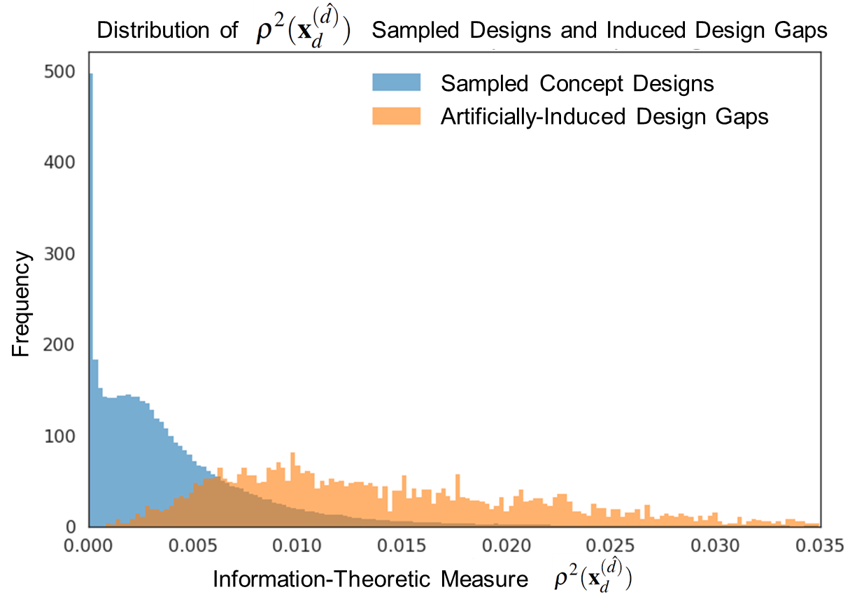
Figure 2: Distribution of $\rho^{2}(\mathbf{x}_{d}^{(\hat{d})})$ for the induced design gaps (orange), and sampled designs $\mathbf{x}_{d}^{(\hat{d})}$. Note that this histogram is normalized, with many more sampled concepts that induced design gaps.

4.2.1 Parameter Estimation

Maximizing the likelihood of of our model given the data as described in Equation (9) requires balancing several factors. First, there is an inherent trade off between the choice model and the desired probabilistic design representation. Specifically, imposing structure on the design feature representation $q(\mathbf{h}_{d}|\mathbf{x}_{d})$ through the $\mathcal{D}_{KL}\left[q(\mathbf{h}_{d}|\mathbf{x}_{d})||p(\mathbf{h}_{d})\right]$ term counteracts the desire of the choice model $p(\mathbf{y}|\mathbf{h}_{c},\mathbf{h}_{d})$ to have a complex unknown distribution over $\mathbf{h}_{d}$ in order to better predict consumer choice. The results in convergence issues if these seperate terms are not balanced during model estimation. We accordingly introduce additional model estimation hyperparameters $\lambda_{1}$ for $\mathcal{D}_{KL}\left[q(\mathbf{h}_{d}|\mathbf{x}_{d})||p(\mathbf{h}_{d})\right]$ within the likelihood optimization objection function.

The architecture of the combined deep learning model is considered a hyperparameter, and several deep architectures were iterated over using the training and validation sets. The combined deep learning model was trained using several first-order optimizers, including including ADAM [17] and plain stochastic gradient descent [35], as various portions of the model required different learning rates and parameter freezing.

Due to the heterogeneity of variable types (i.e., real, binary, categorical), as well as the heteroscadecity in our variables (i.e., vehicle price range) even after training/validation scaled normalization, several constraints were imposed during model parameter estimation (e.g., minimum estimated variance of $\boldsymbol{\sigma}_{d}^{2}\boldsymbol{I}$). All experiments were CPU multithreaded and distributed across multiple GPUs using a single workstation with 128 GB ram, 32 CPU threads at 4.0 GHz, and four Titan XP GPUs.

Choice Prediction Task	Top-1 Acc. (std. dev.)	Top-5 Acc. (std. dev.)	Random
Existing Designs	83.10% (0.86%)	98.21% (0.32%)	0.34%
Nonexisting Designs	76.06% (0.97%)	97.30% (0.12%)	0.37%

Table 1: Consumer choice model prediction accuracies using held-out consumers. Note that “nonexisting” designer refers to holding out any data containing that design (e.g., all Toyota Corollas).

4.2.2 Evaluation Metrics

We aim to predict the exact vehicle the consumer purchases. The consumer choice model is accordingly assessed using ‘Top-1’ and ‘Top-5” evaluation metrics, where ‘Top-1’ refers to how accurately the choice model predicts the exact purchased vehicle, and ‘Top-5’ refers to whether the purchased vehicle is in the choice model’s top five predictions. Assuming a uniform marginal distribution of purchase amongst the designs, the random chance of correct prediction is either $\frac{1}{297}=0.34\%$, or $\frac{1}{268}=0.37\%$. Note that in the latter case, while we hold-in $D=267$, we validate by assuming that only one artificially induced design gap (i.e., the held-out customer’s actual purchase) enters the market.

To assess the design feasibility model, we use the average negative log-likelihood (NLL) given by the generative density learned by the $2^{nd}$ through $4^{th}$ lines in Equation (9) on held-out portions of the designs.

Predicting design gaps is not straightforward. We can not, for example, know whether the design gap sampler given in Algorithm 1 is giving false positives (i.e., no design gap), or true positives that in the past never had a design. Accordingly, we assume that the only design gaps in the market are those that we can observe using the artificially induced design gaps from the actual held-out designs. At the same time, we also assume that every held-out design actually was a design gap (i.e., no products failed). This assumption invokes the notion that the U.S. automotive market is relatively mature, and is dominated by a small set of incumbent players with vast resources, design intuition, and capability to act on such intuition.

Given these constraints, we use an evaluation metric that assesses how well the design gap sampler locates designs relative to other sampled design from the estimated feasible space of designs. Given the multivariate Gaussian assumption on this space, we use the mean-squared-difference metric (MSqE).

Design Feasibility Prediction Task	NLL (std. dev.)
Existing Designs	2621.88 (-)
Nonexisting Designs	2220.03 (-)

Table 2: Negative log likelihood of generative density given design.

4.3 Results

Prediction accuracies for held-out consumers are given in Table 1. Standard deviations are calculated on 3 experiments with the same held-out vehicles. Standard deviations are likely larger given more computational run time for splits with different held-out vehicles.

Design Gap Prediction	MSqE (std. dev.)
Random Feasible Design	0.263 (0.000412)
Predicted Gap	0.251

Table 3: Mean-squared error between predicted design gaps and randomly sampled designs.

The evaluation of the design feasibility model is given in Table 2. We note that lower NLL on held-out designs is likely due to the lower entropy of the these data relative to the learned density. For example, our random split of testing data did not include designs such as $\frac{1}{2}$-ton trucks or sports convertibles. Further computational runtime with holding out different random vehicles may lead to different results.

Design gap distances between the artificially induced design gaps, and the concept designs $\mathbf{x}_{d}^{(\hat{d})}$ sampled by Algorithm 1 are given in Table 3. Random feasible design refers to any concept design sampled, while ‘Predicted Gap’ refers to concept designs that were predicted at minimum to have $\rho^{2}(\mathbf{x}_{d}^{(\hat{d})})\geq\gamma_{2}$ . We give standard deviations to show the relative scale of this space. In short, in high-dimensional spaces, all distances looks roughly the same [1]. Furthermore, in Figure (2) we plot the distribution of $\rho^{2}(\cdot)$ for both sampled concept designs $\mathbf{x}_{d}^{(\hat{d})}$ and held-out artificially induced design gaps.

5 Discussion and Future Work

While this work is preliminary, the results give evidence that this approach may have potential for predicting design gaps. This is suggested by the lower mean-squared distance of sampled design concepts $\mathbf{x}_{d}^{(\hat{d})}$ with $\rho^{2}(\mathbf{x}_{d}^{(\hat{d})})\geq\gamma_{2}$ relative to those without rejection. This result in itself, however, is not sufficient to claim prediction of design gaps. These distance calculations are ultimately being performed in an approximate representation of a multivariate Gaussian, which is already being estimated using deep learning models. Deep learning models, while recently state-of-the-art for many prediction tasks, are known to be “brittle” in their predictions [10]. This can lead to warping of the design space that lead to unreasonable distance calculations, particularly given our prediction regime of held-out customers, held-out designs, and unknown design gaps.

At the same time, these results in conjunction with the very strong prediction results by the consumer choice model given in Table 1 do suggest that this approach may have have potential for more direct estimation of design gaps. Given the implications of a validated method to help product design and market opportunities potentially years in advance, without requiring a priori knowledge possible design concepts, further study is warranted.

Accordingly, there are significant opportunities for future work. Perhaps the portion of this approach with most opportunity for improvement lies in the search method of the bounded design space. The sampling method given in Algorithm 1, like many sampling algorithms, is computationally inefficient due to the high-dimensionality space the samples are drawn samples (even after dimensionality reduction from the original design variable representation). With better validation on the structure of the feature space, optimization methods would likely prove to be a significantly more computationally efficient means of searching the space of possible designs for design gaps.

This opportunity to perform optimization over this space perhaps deserves attention on its own. In short, this is enabled by the magnitude of prediction accuracy obtained by the deep consumer choice model. This work builds off previously conducted work by the authors also in vehicle purchase prediction [7], in which the task was of more conventional binary choice conjoint analysis. We note that in the previous study, an accuracy of $75.15\%$ was achieved by the model most conceptually similar to that in this work. However, in the previous study $50\%$ represented random chance while in this study, random chance is effectively $0\%$. These two tasks are best conceptually comparable if we were to decompose each multinomial prediction to all pairwise comparisons. A consumer choice model that has less than 50% accuracy on average for all pairwise design comparisons will always lead to suboptimal design.

As earlier noted with regards to distance metrics, efficiently searching the design space using optimization also requires well-behaved probabilistic structure imposed on the design feature space. This comes with a cost of (potentially significantly) reducing the predictive accuracy of the consumer choice model. This tradeoff thus warrants further study. Lastly, any future improvement and even development of this approach should necessitate “real” validation for actual usage. In other words, without using data alone, controlled experiments should be conducted to with new consumers to assess to validity of this approach.

6 Conclusion

In this work we introduce a deep learning approach to predict design gaps by learning a consumer choice model as well as a design feasibility model. This approach builds on conventions in both quantitative marketing in bounding the heterogeneity of consumer choice preferences, as well as engineering design for bounding the space of possible designs. We further introduce variational approximations to induce desired probabilistic structure in the space of possible designs, as well as making this model amenable for efficient parameter estimation using recent advances in machine learning. Our approach is tested on a large dataset of real design purchases in the U.S. automotive market. While our work is preliminary, we find that evidence that with sufficiently accurate consumer choice and design constraint models, it may be possible to predict design gaps in the market that do not need to be specified beforehand.

References

- [1] Charu C. Aggarwal, Alexander Hinneburg, and Daniel A. Keim. On the Surprising Behavior of Distance Metrics in High Dimensional Space. In Gerhard Goos, Juris Hartmanis, Jan van Leeuwen, Jan Van den Bussche, and Victor Vianu, editors, Database Theory — ICDT 2001, volume 1973, pages 420–434. Springer Berlin Heidelberg, Berlin, Heidelberg, 2001.
- [2] Greg M. Allenby and Peter E. Rossi. Marketing models of consumer heterogeneity. Journal of econometrics, 89(1):57–78, 1998.
- [3] Alparslan Emrah Bayrak, Yi Ren, and Panos Y. Papalambros. Design of Hybrid-Electric Vehicle Architectures Using Auto-Generation of Feasible Driving Modes. page V001T01A005. ASME, August 2013.
- [4] Michael Braun and Jon McAuliffe. Variational Inference for Large-Scale Models of Discrete Choice. Journal of the American Statistical Association, 105(489):324–335, March 2010.
- [5] Egon Brunswik. The conceptual framework of psychology. Psychological Bulletin, 49(6):654–656, 1952.
- [6] Alex Burnap, Jeffrey Hartley, Yanxin Pan, Richard Gonzalez, and Panos Y. Papalambros. Balancing design freedom and brand recognition in the evolution of automotive brand styling. Design Science Journal, 2(9), 2016.
- [7] Alex Burnap, Yanxin Pan, Ye Liu, Yi Ren, Honglak Lee, Richard Gonzalez, and Panos Y. Papalambros. Improving Design Preference Prediction Accuracy Using Feature Learning. Journal of Mechanical Design, 138(7):071404, 2016.
- [8] Alexander Burnap. Crowdsourcing for Engineering Design: Objective Evaluations and Subjective Preferences. 8 2016.
- [9] Theodoros Evgeniou, Constantinos Boussios, and Giorgos Zacharia. Generalized robust conjoint estimation. Marketing Science, 24(3):415–429, 2005.
- [10] Ian J. Goodfellow, Jonathon Shlens, and Christian Szegedy. Explaining and Harnessing Adversarial Examples. arXiv:1412.6572 [cs, stat], December 2014.
- [11] EJ Gumbel. Statistics of extremes. 1958. Columbia Univ. press, New York, page 247, 1958.
- [12] John R Hauser. Testing the accuracy, usefulness, and significance of probabilistic choice models: An information-theoretic approach. Operations Research, 26(3):406–421, 1978.
- [13] John R Hauser, Olivier Toubia, Theodoros Evgeniou, Rene Befurt, and Daria Dzyabura. Disjunctions of Conjunctions, Cognitive Simplicity, and Consideration Sets. Journal of Marketing Research, 47(3):485–496, June 2010.
- [14] George A. Hazelrigg. A framework for decision-based engineering design. Journal of mechanical design, 120(4):653–658, 1998.
- [15] Harald Hruschka. Analyzing market baskets by restricted Boltzmann machines. OR Spectrum, 36(1):209–228, January 2014.
- [16] Daniel Kahneman. Maps of bounded rationality: Psychology for behavioral economics. The American economic review, 93(5):1449–1475, 2003.
- [17] Diederik P. Kingma and Jimmy Ba Adam. Adam: A method for stochastic optimization. In International Conference on Learning Representation, San Diego, California, 2015.
- [18] Diederik P Kingma, Shakir Mohamed, Danilo Jimenez Rezende, and Max Welling. Semi-supervised Learning with Deep Generative Models. pages 3581–3589, 2014.
- [19] Diederik P. Kingma and Max Welling. Auto-encoding variational bayes. arXiv preprint arXiv:1312.6114, 2013.
- [20] Oleg Korenok, George E. Hoffer, and Edward L. Millner. Non-price determinants of automotive demand: Restyling matters most. Journal of Business Research, 63(12):1282–1289, December 2010.
- [21] V. Krishnan and Karl T. Ulrich. Product Development Decisions: A Review of the Literature. Management Science, 47(1):1–21, January 2001.
- [22] Peter J. Lenk, Wayne S. DeSarbo, Paul E. Green, and Martin R. Young. Hierarchical Bayes Conjoint Analysis: Recovery of Partworth Heterogeneity from Reduced Experimental Designs. Marketing Science, 15(2):173–191, 1996.
- [23] Kemper E. Lewis, Wei Chen, and Linda C. Schmidt, editors. Decision Making in Engineering Design. ASME, Three Park Avenue New York, NY 10016-5990, January 2006.
- [24] Liu Liu and Daria Dzyabura. Capturing Multi-taste Preferences: A Machine Learning Approach. 2016.
- [25] Minhua Long and W. Ross Morrow. Should Optimal Designers Worry About Consideration? Journal of Mechanical Design, 137(7):071411, 2015.
- [26] R Duncan Luce. Individual choice behavior: A theoretical analysis. Courier Corporation, 1959.
- [27] Jeremy J Michalek, Fred M Feinberg, and Panos Y Papalambros. Linking Marketing and Engineering Product Design Decisions via Analytical Target CascadingÃ. page 21.
- [28] Andriy Mnih and Ruslan Salakhutdinov. Probabilistic matrix factorization. In Advances in neural information processing systems, pages 1257–1264, 2007.
- [29] Patricia L Mokhtarian. Discrete choice models’ : A reintroduction to an old friend. Journal of choice modelling, 21:60–65, 2016.
- [30] W. Ross Morrow, Minhua Long, and Erin F. MacDonald. Market-System Design Optimization With Consider-Then-Choose Models. Journal of Mechanical Design, 136(3):031003, 2014.
- [31] Donald A. Norman. Emotional Design: Why We Love (or Hate) Everyday Things. Basic books, New York, NY, 2004.
- [32] Donald A. Norman, Andrew Ortony, and Daniel M. Russell. Affect and machine design: Lessons for the development of autonomous machines. IBM Systems Journal, 42(1):38–44, 2003.
- [33] Bryan K Orme. Getting started with conjoint analysis: strategies for product design and pricing research. Research Publishers, 2010.
- [34] Takayuki Osogami and Makoto Otsuka. Restricted Boltzmann machines modeling human choice. In Advances in Neural Information Processing Systems, pages 73–81, 2014.
- [35] Panos Y. Papalambros and Douglass J. Wilde. Principles of optimal design: modeling and computation. Cambridge university press, 2000.
- [36] John W. Payne. Task complexity and contingent processing in decision making: An information search and protocol analysis. Organizational Behavior and Human Performance, 16(2):366–387, August 1976.
- [37] Marta Perez Mata, Saeema Ahmed-Kristensen, and Kristina Shea. Spatial Grammar for Design Synthesis Targeting Perceptions: Case Study on Beauty. page V01AT02A013, August 2015.
- [38] Max Yi Ren and Clayton Scott. Adaptive questionnaires for direct identification of optimal product design. arXiv preprint arXiv:1701.01231, 2017.
- [39] Peter E. Rossi and Greg M. Allenby. Bayesian statistics and marketing. Marketing Science, 22(3):304–328, 2003.
- [40] Peter E. Rossi, Robert E. McCulloch, and Greg M. Allenby. The value of purchase history data in target marketing. Marketing Science, 15(4):321–340, 1996.
- [41] Ruslan Salakhutdinov, Andriy Mnih, and Geoffrey Hinton. Restricted Boltzmann machines for collaborative filtering. In Proceedings of the 24th international conference on Machine learning, pages 791–798. ACM, 2007.
- [42] N. Siddharth, Brooks Paige, Jan-Willem van de Meent, Alban Desmaison, Noah D. Goodman, Pushmeet Kohli, Frank Wood, and Philip H. S. Torr. Learning Disentangled Representations with Semi-Supervised Deep Generative Models. arXiv:1706.00400 [cs, stat], June 2017. arXiv: 1706.00400.
- [43] Vishal Singh and Ning Gu. Towards an integrated generative design framework. Design Studies, 33(2):185–207, March 2012.
- [44] Louis Thurstone. The method of paired comparisons for social values. The Journal of Abnormal and Social Psychology, 21(4), 1927.
- [45] Olivier Toubia, Duncan Simester, and John R. Hauser. Fast Polyhedral Adaptive Conjoint Estimation. SSRN Electronic Journal, 2001.
- [46] Suppawong Tuarob and Conrad S. Tucker. A product feature inference model for mining implicit customer preferences within large scale social media networks. In ASME 2015 International Design Engineering Technical Conferences and Computers and Information in Engineering Conference, pages V01BT02A002–V01BT02A002. American Society of Mechanical Engineers, 2015.
- [47] Amos Tversky. Elimination by Aspects: A Theory of Choice l. page 19.
- [48] Amos Tversky. Intransitivity of preferences. 76(1), 1969.
- [49] Alice M Tybout and John R. Hauser. A marketing audit using a conceptual model of consumer behavior: Application and evaluation. Journal of Marketing, pages 82–101, 1981.
- [50] David Van Horn, Andrew Olewnik, and Kemper Lewis. Design analytics: capturing, understanding, and meeting customer needs using big data. In ASME 2012 International Design Engineering Technical Conferences and Computers and Information in Engineering Conference, pages 863–875. American Society of Mechanical Engineers, 2012.
- [51] John Von Neumann and Oskar Morgenstern. Theory of games and economic behavior. Princeton university press, 1944.
- [52] Henk Jan Wassenaar, Wei Chen, Jie Cheng, and Agus Sudjianto. Enhancing discrete choice demand modeling for decision-based design. Journal of Mechanical Design, 127(4):514–523, 2005.
- [53] Michel Wedel and Wagner A. Kamakura. Market segmentation: Conceptual and methodological foundations, volume 8. Springer Science & Business Media, 2012.