Efficient energy-preserving methods for charged-particle dynamics

Abstract

In this paper, energy-preserving methods are formulated and studied for solving charged-particle dynamics. We first formulate the scheme of energy-preserving methods and analyze its basic properties including algebraic order and symmetry. Then it is shown that these novel methods can exactly preserve the energy of charged-particle dynamics. Moreover, the long time momentum conservation is studied along such energy-preserving methods. A numerical experiment is carried out to illustrate the notable superiority of the new methods in comparison with the popular Boris method in the literature.

Keywords: Charged particle dynamics; Energy-preserving methods; Long-time conservtion

MSC (2000): 65P10, 65L05

1 Introduction

A large amount of work in the literature has been devoted to studying the following charged-particle dynamics (see, e.g. [1, 2, 6, 10, 14, 15, 17, 26, 27, 33])

$$\ddot{x}=\dot{x}\times B(x)+F(x),\ \ \ \ \ x(t_{0})=x^{0},\ \ \dot{x}(t_{0})=\dot{x}^{0}$$ (1)

where $x(t)\in{\mathbb{R}}^{3}$ represents the position of a particle moving in an electro-magnetic field, $B(x)$ is a magnetic field which is defined as $B(x)=\nabla_{x}\times A(x)$ with the vector potential $A(x)\in{\mathbb{R}}^{3}$, and $F(x)$ is the negative gradient of the scalar potential $U(x)$. We define $v=\dot{x}$ and then the energy of the dynamics is given by

$$E(x,v)=\frac{1}{2}\left|v\right|^{2}+U(x).$$ (2)

It is well known that the solution of this system conserves the energy exactly, i.e.

$$E(x(t),v(t))\equiv E(x^{0},\dot{x}^{0})\ \ \ \textmd{for\ any }t.$$

It has been shown in [14] that if the $U(x)$ and $A(x)$ have the following properties

$$U(e^{\tau S}x)=U(x)\ \ \textmd{and }\ \ e^{-\tau S}A(e^{\tau S}x)=A(x)\ \ \ \ \ \textmd{for\ \ all\ \ real}\ \ \tau,$$ (3)

where $S$ is a skew-symmetric matrix, then the momentum

$$M(x,v)=(v+A(x))^{\intercal}Sx$$ (4)

is conserved along the solution of the differential equation (1). This point can be proved by multiplying (1) with $Sx$ and the reader is referred to [14] for details. It has also been noted in [14] that since the matrix $S$ is skew-symmetric, we have $x^{\intercal}S\ddot{x}=-\frac{d}{dt}(x^{\intercal}S\dot{x})$ and it follows from these properties that $S\nabla U(x)=0$ and $x^{\intercal}S(\dot{x}\times B(x))=-\frac{d}{dt}(x^{\intercal}SA(x)).$

In this paper, we denote the vector $B(x)$ by $B(x)=(B_{1}(x),B_{2}(x),B_{3}(x))^{\intercal}$, where $B_{i}(x)\in{\mathbb{R}}$ for $i=1,2,3.$ By the definition of the cross product, we obtain $\dot{x}\times B(x)=\tilde{B}(x)\dot{x},$ where the skew-symmetric matrix $\tilde{B}(x)$ is given by

$$\tilde{B}(x)=\left(\begin{array}[]{ccc}0&B_{3}(x)&-B_{2}(x)\\ -B_{3}(x)&0&B_{1}(x)\\ B_{2}(x)&-B_{1}(x)&0\\ \end{array}\right).$$

In order to solve the charged-particle dynamics effectively, many kinds of useful methods have been studied and developed. Boris method [2] is a popular integrator and it was researched further in [10, 14, 26]. There are many other kinds of methods which have been researched for solving charged-particle dynamics, such as volume-preserving algorithms in [17], symmetric multistep methods in [15] and symplectic or K-symplectic integrators in [27, 33]. Recently, the authors in [20] proposed adapted exponential integrators for solving charged-particle dynamics and analyzed its symplecticity.

On the other hand, energy-preserving methods are an important and efficient kind of methods which have been received much attention in the past few years. The authors in [11] constructed energy-preserving $B$-series methods. The Average Vector Field (AVF) method was presented in [8, 9] and it was shown in [25] that AVF method is also a $B$-series method. In [29], the authors proposed a new trigonometric energy-preserving method. Various different kinds of energy-preserving methods are proposed and analyzed, such as discrete gradient methods (see, e.g. [23, 30]), the energy-preserving exponentially-fitted methods(see, e.g. [21, 22]), time finite elements methods (see, e.g. [3, 18]), the Runge-Kutta-type energy-preserving collocation methods(see, e.g. [7, 13]) and Hamiltonian Boundary Value Methods ( see, e.g. [4]). We refer to [19, 24, 25, 28, 31, 32] for more research work on energy-preserving methods. However, it seems that energy-preserving methods for solving charged-particle dynamics have not been considered in the literature, which motivates this paper.

Based on these work, we will formulate and research a novel energy-preserving method for solving charged-particle dynamics (1). The rest of this paper is organized as follows. In Section 2, we present the scheme of the method and analyze its algebraic order and symmetry. In Section 3, it is shown that the novel method can exactly preserve the energy (2) of charged-particle dynamics. The long time near conservation of the momentum for this new method is discussed in Section 4. Section 5 reports a numerical experiment to show the efficiency of the novel method. Section 6 is devoted to the conclusions of this paper.

2 The scheme of the method and its basic properties

2.1 Formulation of the method

In order to drive effective methods for the system (1), we first present its exact solution by the variation-of-constants formula.

Theorem 2.1

(See [16].) The exact solution of (1) can be expressed as

$$\begin{array}[c]{ll}&x(t_{n}+h)=x(t_{n})+hv(t_{n})+h^{2}\int_{0}^{1}(1-z)\hat{f}(t_{n}+hz)dz,\\ &v(t_{n}+h)=v(t_{n})+h\int_{0}^{1}\hat{f}(t_{n}+hz)dz,\end{array}$$ (5)

where $\hat{f}(t):=\tilde{B}(x(t))v(t)+F(x(t))$.

Based on the variation-of-constants formula, we define the following method for the charged-particle dynamics (1).

Definition 2.2

The energy-preserving method for solving charged-particle dynamics (1) is defined as

$$\begin{array}[c]{ll}&x_{n+1}=x_{n}+hv_{n}+\frac{h^{2}}{2}\int_{0}^{1}F(x_{n}+\tau(x_{n+1}-x_{n}))d\tau+\frac{h^{2}}{2}\tilde{B}(\frac{x_{n+1}+x_{n}}{2})\frac{v_{n+1}+v_{n}}{2},\\ &v_{n+1}=v_{n}+h\int_{0}^{1}F(x_{n}+\tau(x_{n+1}-x_{n}))d\tau+h\tilde{B}(\frac{x_{n+1}+x_{n}}{2})\frac{v_{n+1}+v_{n}}{2},\end{array}$$ (6)

where $h$ is a stepsize. We denote this method by EP.

2.2 Algebraic order

Theorem 2.3

Under the local assumptions $x(t_{n})=x_{n}$ and $v(t_{n})=v_{n}$, the energy-preserving method (6) is of order two, i.e.,

$$x(t_{n+1})-x_{n+1}=\mathcal{O}(h^{3}),\ \ \ \ \ \ \ v(t_{n+1})-v_{n+1}=\mathcal{O}(h^{3}).$$

Proof  By (5) and (6), we compute

$$\begin{array}[c]{lll}&x(t_{n+1})-x_{n+1}\\ =&(x(t_{n})+hv(t_{n})+h^{2}\int_{0}^{1}(1-z)\hat{f}(t_{n}+hz)dz)\\ &-(x_{n}+hv_{n}+\frac{h^{2}}{2}\int_{0}^{1}F(x_{n}+\tau(x_{n+1}-x_{n}))d\tau+\frac{h^{2}}{2}\tilde{B}(\frac{x_{n+1}+x_{n}}{2})\frac{v_{n+1}+v_{n}}{2})\\ =&(x(t_{n})+hv(t_{n})+h^{2}\int_{0}^{1}(1-z)\tilde{B}(x(t_{n}+hz))v(t_{n}+hz)dz+h^{2}\int_{0}^{1}(1-z)F(x(t_{n}+hz))dz)\\ &-(x_{n}+hv_{n}+\frac{h^{2}}{2}\int_{0}^{1}F(x_{n}+\tau(x_{n+1}-x_{n}))d\tau+\frac{h^{2}}{2}\tilde{B}(\frac{x_{n+1}+x_{n}}{2})\frac{v_{n+1}+v_{n}}{2})\\ =&h^{2}(\int_{0}^{1}(1-z)\tilde{B}(x(t_{n}))v(t_{n})dz+\mathcal{O}(h)+\int_{0}^{1}(1-z)F(x(t_{n}))dz+\mathcal{O}(h))\\ &-(\frac{h^{2}}{2}\int_{0}^{1}F(x_{n}+\tau(x_{n+1}-x_{n}))d\tau+\frac{h^{2}}{2}\tilde{B}(\frac{x_{n+1}+x_{n}}{2})\frac{v_{n+1}+v_{n}}{2})\\ =&h^{2}\int_{0}^{1}(1-z)\tilde{B}(x_{n})v_{n}dz+h^{2}\int_{0}^{1}(1-z)F(x_{n})dz-\frac{h^{2}}{2}\tilde{B}(\frac{x_{n+1}+x_{n}}{2})\frac{v_{n+1}+v_{n}}{2}\\ &-\frac{h^{2}}{2}\int_{0}^{1}F(x_{n}+\tau(x_{n+1}-x_{n}))d\tau+\mathcal{O}(h^{3})\\ =&\frac{h^{2}}{2}(\tilde{B}(x_{n})v_{n}-\tilde{B}(\frac{x_{n+1}+x_{n}}{2})\frac{v_{n+1}+v_{n}}{2})+\frac{h^{2}}{2}(F(x_{n})-\int_{0}^{1}F(x_{n}+\tau(x_{n+1}+x_{n}))d\tau)+\mathcal{O}(h^{3}).\end{array}$$ (7)

In the light of $x_{n+1}=x_{n}+\mathcal{O}(h)$ and $v_{n+1}=v_{n}+\mathcal{O}(h),$ it is obtained that

$$\tilde{B}(\frac{x_{n+1}+x_{n}}{2})\frac{v_{n+1}+v_{n}}{2}=\tilde{B}(x_{n})v_{n}+\mathcal{O}(h).$$

On the other hand, we have

$$\int_{0}^{1}F(x_{n}+\tau(x_{n+1}+x_{n}))d\tau=F(x_{n})+\mathcal{O}(h).$$

Consequently, the formula (7) becomes

$$x(t_{n+1})-x_{n+1}=\mathcal{O}(h^{3}).$$

Similarly, we obtain $v(t_{n+1})-v_{n+1}=\mathcal{O}(h^{3}).$ The proof is complete.

2.3 Symmetry of the method

A numerical method denoted by $y_{n+1}=\Phi_{h}(y_{n})$ is called to be symmetric if exchanging $y_{n}\leftrightarrow y_{n+1}$ and $h\leftrightarrow-h$ does not change the scheme of the method (see [16]). It has been pointed out in [16] that symmetric methods have excellent longtime behaviour and they play an important role in geometric numerical integration.

Theorem 2.4

The method (6) is symmetric.

Proof  Exchanging $x_{n}\leftrightarrow x_{n+1},v_{n}\leftrightarrow v_{n+1}$ and $h\leftrightarrow-h$ in (6) yields

$$\begin{array}[c]{ll}&x_{n}=x_{n+1}-hv_{n+1}+\frac{h^{2}}{2}\int_{0}^{1}F(x_{n+1}+\tau(x_{n}-x_{n+1}))d\tau+\frac{h^{2}}{2}\tilde{B}(\frac{x_{n}+x_{n+1}}{2})\frac{v_{n}+v_{n+1}}{2},\\ &v_{n}=v_{n+1}-h\int_{0}^{1}F(x_{n+1}+\tau(x_{n}-x_{n+1}))d\tau-h\tilde{B}(\frac{x_{n}+x_{n+1}}{2})\frac{v_{n}+v_{n+1}}{2}.\end{array}$$ (8)

From formula (8), it follows that

$$\begin{array}[c]{ll}&x_{n+1}=x_{n}+hv_{n}+\frac{h^{2}}{2}\int_{0}^{1}F(x_{n+1}+\tau(x_{n}-x_{n+1}))d\tau+\frac{h^{2}}{2}\tilde{B}(\frac{x_{n+1}+x_{n}}{2})\frac{v_{n+1}+v_{n}}{2},\\ &v_{n+1}=v_{n}+h\int_{0}^{1}F(x_{n+1}+\tau(x_{n}-x_{n+1}))d\tau+h\tilde{B}(\frac{x_{n+1}+x_{n}}{2})\frac{v_{n+1}+v_{n}}{2}.\end{array}$$ (9)

Letting $\sigma=1-\tau$ yields

$$\begin{array}[c]{ll}&\int_{0}^{1}F(x_{n+1}+\tau(x_{n}-x_{n+1}))d\tau=\int_{0}^{1}F(x_{n}+(1-\tau)(x_{n+1}-x_{n}))d\tau\\ &=-\int_{1}^{0}F(x_{n}+\sigma(x_{n+1}-x_{n}))d\sigma=\int_{0}^{1}F(x_{n}+\tau(x_{n+1}-x_{n}))d\tau.\end{array}$$

which shows that (9) is the same as (6). Therefore, the method (6) is symmetric.

3 Energy-preserving property

In this section, we show the energy-preserving property of the method (6).

Theorem 3.1

The method (6) preserves the energy $E$ in (2) exactly, i.e.,

$$E(x_{n+1},v_{n+1})=E(x_{n},v_{n})\ \ \ \ \ for\ \ \ \ n=0,1,\ldots$$

Proof  In this paper, we denote $\digamma:=\int_{0}^{1}F(x_{n}+\tau(x_{n+1}-x_{n}))d\tau$. We compute

$$E(x_{n+1},v_{n+1})=\frac{1}{2}v_{n+1}^{\intercal}v_{n+1}+U(x_{n+1}).$$ (10)

Keeping the fact in mind that $\tilde{B}(x)$ is skew-symmetric and inserting the second formula of (6) into (10) yields

$$\begin{array}[c]{llll}&E(x_{n+1},v_{n+1})\\ =&\frac{1}{2}(v_{n}+h\digamma+h\tilde{B}(\frac{x_{n+1}+x_{n}}{2})\frac{v_{n+1}+v_{n}}{2})^{\intercal}(v_{n}+h\digamma+h\tilde{B}(\frac{x_{n+1}+x_{n}}{2})\frac{v_{n+1}+v_{n}}{2})+U(x_{n+1})\\ =&\frac{1}{2}v_{n}^{\intercal}v_{n}+\frac{h}{2}v_{n}^{\intercal}\digamma+\frac{h}{4}v_{n}^{\intercal}\tilde{B}(\frac{x_{n+1}+x_{n}}{2})(v_{n+1}+v_{n})+\frac{h}{2}\digamma^{\intercal}v_{n}+\frac{h^{2}}{2}\digamma^{\intercal}\digamma+\frac{h^{2}}{4}\digamma^{\intercal}\tilde{B}(\frac{x_{n+1}+x_{n}}{2})(v_{n+1}+v_{n})\\ &-\frac{h}{4}(v_{n+1}+v_{n})^{\intercal}\tilde{B}(\frac{x_{n+1}+x_{n}}{2})v_{n}-\frac{h^{2}}{8}(v_{n+1}+v_{n})^{\intercal}\tilde{B}(\frac{x_{n+1}+x_{n}}{2})\tilde{B}(\frac{x_{n+1}+x_{n}}{2})(v_{n+1}+v_{n})\\ &-\frac{h^{2}}{4}(v_{n+1}+v_{n})^{\intercal}\tilde{B}(\frac{x_{n+1}+x_{n}}{2})\digamma+U(x_{n+1})\\ =&\frac{1}{2}v_{n}^{\intercal}v_{n}+\frac{h}{2}v_{n}^{\intercal}\digamma+\frac{h}{2}v_{n}^{\intercal}\tilde{B}(\frac{x_{n+1}+x_{n}}{2})(v_{n+1}+v_{n})+\frac{h}{2}\digamma^{\intercal}v_{n}+\frac{h^{2}}{2}\digamma^{\intercal}\digamma+\frac{h^{2}}{2}\digamma^{\intercal}\tilde{B}(\frac{x_{n+1}+x_{n}}{2})(v_{n+1}+v_{n})\\ &-\frac{h^{2}}{8}(v_{n+1}+v_{n})^{\intercal}\tilde{B}(\frac{x_{n+1}+x_{n}}{2})\tilde{B}(\frac{x_{n+1}+x_{n}}{2})(v_{n+1}+v_{n})+U(x_{n+1}).\end{array}$$ (11)

On the other hand, we have

$$\begin{array}[c]{ll}&U(x_{n})-U(x_{n+1})=-\int_{0}^{1}dU((1-\sigma)x_{n}+\sigma x_{n+1})\\ &=-\int_{0}^{1}(x_{n+1}-x_{n})^{\intercal}\nabla_{x}U((1-\sigma)x_{n}+\sigma x_{n+1})d\sigma=\digamma^{\intercal}(x_{n+1}-x_{n})\\ &=\frac{h}{2}\digamma^{\intercal}v_{n+1}+\frac{h}{2}\digamma^{\intercal}v_{n}.\end{array}$$

Inserting this result into (11) implies

$$\begin{array}[c]{llll}&E(x_{n+1},v_{n+1})\\ =&\frac{1}{2}v_{n}^{\intercal}v_{n}+\frac{h}{2}v_{n}^{\intercal}\digamma+\frac{h}{2}v_{n}^{\intercal}\tilde{B}(\frac{x_{n+1}+x_{n}}{2})(v_{n+1}+v_{n})+\frac{h}{2}\digamma^{\intercal}v_{n}+\frac{h^{2}}{2}\digamma^{\intercal}\digamma\\ &+\frac{h^{2}}{2}\digamma^{\intercal}\tilde{B}(\frac{x_{n+1}+x_{n}}{2})(v_{n+1}+v_{n})-\frac{h^{2}}{8}(v_{n+1}+v_{n})^{\intercal}\tilde{B}(\frac{x_{n+1}+x_{n}}{2})\tilde{B}(\frac{x_{n+1}+x_{n}}{2})(v_{n+1}+v_{n})\\ &+U(x_{n})-\frac{h}{2}\digamma^{\intercal}v_{n+1}-\frac{h}{2}\digamma^{\intercal}v_{n}\\ =&\frac{1}{2}v_{n}^{\intercal}v_{n}+U(x_{n})+\frac{h}{2}v_{n}^{\intercal}\digamma+\frac{h}{2}v_{n}^{\intercal}\tilde{B}(\frac{x_{n+1}+x_{n}}{2})(v_{n+1}+v_{n})+\frac{h^{2}}{2}\digamma^{\intercal}\digamma-\frac{h}{2}\digamma^{\intercal}v_{n+1}\\ &+\frac{h^{2}}{2}\digamma^{\intercal}\tilde{B}(\frac{x_{n+1}+x_{n}}{2})(v_{n+1}+v_{n})-\frac{h^{2}}{8}(v_{n+1}+v_{n})^{\intercal}\tilde{B}(\frac{x_{n+1}+x_{n}}{2})\tilde{B}(\frac{x_{n+1}+x_{n}}{2})(v_{n+1}+v_{n}).\end{array}$$ (12)

According to the second formula of (6), it follows that

$$\begin{array}[c]{ll}\digamma^{\intercal}v_{n+1}&=\digamma^{\intercal}(v_{n}+h\digamma+\frac{h}{2}\tilde{B}(\frac{x_{n+1}+x_{n}}{2})(v_{n+1}+v_{n}))\\ &=\digamma^{\intercal}v_{n}+h\digamma^{\intercal}\digamma+\frac{h}{2}\digamma^{\intercal}\tilde{B}(\frac{x_{n+1}+x_{n}}{2})(v_{n+1}+v_{n}).\end{array}$$

Thus, (12) becomes

$$\begin{array}[c]{llll}&E(x_{n+1},v_{n+1})\\ =&\frac{1}{2}v_{n}^{\intercal}v_{n}+U(x_{n})+\frac{h}{2}v_{n}^{\intercal}\digamma+\frac{h}{2}v_{n}^{\intercal}\tilde{B}(\frac{x_{n+1}+x_{n}}{2})(v_{n+1}+v_{n})\\ &+\frac{h^{2}}{2}\digamma^{\intercal}\digamma-\frac{h}{2}\digamma^{\intercal}v_{n}-\frac{h^{2}}{2}\digamma^{\intercal}\digamma-\frac{h^{2}}{4}\digamma^{\intercal}\tilde{B}(\frac{x_{n}+x_{n+1}}{2})(v_{n+1}+v_{n})\\ &+\frac{h^{2}}{2}\digamma^{\intercal}\tilde{B}(\frac{x_{n+1}+x_{n}}{2})(v_{n+1}+v_{n})-\frac{h^{2}}{8}(v_{n+1}+v_{n})^{\intercal}\tilde{B}(\frac{x_{n+1}+x_{n}}{2})\tilde{B}(\frac{x_{n+1}+x_{n}}{2})(v_{n+1}+v_{n})\\ =&\frac{1}{2}v_{n}^{\intercal}v_{n}+U(x_{n})+\frac{h}{2}(v_{n}^{\intercal}+\frac{h}{2}\digamma^{\intercal}-\frac{h}{4}(v_{n+1}+v_{n})^{\intercal}\tilde{B}(\frac{x_{n+1}+x_{n}}{2}))\tilde{B}(\frac{x_{n+1}+x_{n}}{2})(v_{n+1}+v_{n}).\end{array}$$ (13)

Based on the property of $\tilde{B}(x)$ and the second formula of (6), we obtain

$$-\frac{h}{4}(v_{n+1}+v_{n})^{\intercal}\tilde{B}(\frac{x_{n+1}+x_{n}}{2})=(\frac{h}{4}\tilde{B}(\frac{x_{n+1}+x_{n}}{2})(v_{n+1}+v_{n}))^{\intercal}=\frac{1}{2}v_{n+1}^{\intercal}-\frac{1}{2}v_{n}^{\intercal}-\frac{h}{2}\digamma^{\intercal}.$$

Hence, (13) can be rewritten as

$$\begin{array}[c]{ll}&E(x_{n+1},v_{n+1})\\ =&\frac{1}{2}v_{n}^{\intercal}v_{n}+U(x_{n})+\frac{h}{2}(v_{n}^{\intercal}+\frac{h}{2}\digamma^{\intercal}+\frac{1}{2}v_{n+1}^{\intercal}-\frac{1}{2}v_{n}^{\intercal}-\frac{h}{2}\digamma^{\intercal})\tilde{B}(\frac{x_{n+1}+x_{n}}{2})(v_{n+1}+v_{n})\\ =&\frac{1}{2}v_{n}^{\intercal}v_{n}+U(x_{n})+\frac{h}{4}(v_{n+1}+v_{n})^{\intercal}\tilde{B}(\frac{x_{n+1}+x_{n}}{2})(v_{n+1}+v_{n}).\end{array}$$ (14)

Then, it can be checked that

$$\begin{array}[c]{ll}(\frac{h}{4}(v_{n+1}+v_{n})^{\intercal}\tilde{B}(\frac{x_{n+1}+x_{n}}{2})(v_{n+1}+v_{n}))^{\intercal}=-\frac{h}{4}(v_{n+1}+v_{n})^{\intercal}\tilde{B}(\frac{x_{n+1}+x_{n}}{2})(v_{n+1}+v_{n}),\\ \end{array}$$

which shows that $\frac{h}{4}(v_{n+1}+v_{n})^{\intercal}\tilde{B}(\frac{x_{n+1}+x_{n}}{2})(v_{n+1}+v_{n})=0$. Therefore, (14) becomes

$$E(x_{n+1},v_{n+1})=\frac{1}{2}v_{n}^{\intercal}v_{n}+U(x_{n})=E(x_{n},v_{n}).$$

This implies the statement of the theorem.

We note that the integral in (6) can be evaluated exactly if $U$ is a special function, we have the following theorem.

Theorem 3.2

Assume $U=U(a^{\intercal}x)$ with $a\in\mathbb{R}^{3}$, then

$$\int_{0}^{1}F(x_{n}+\tau(x_{n+1}-x_{n}))d\tau=\frac{-a}{a^{\intercal}x_{n+1}-a^{\intercal}x_{n}}(U(a^{\intercal}x_{n+1})-U(a^{\intercal}x_{n})).$$

Proof  This result is obtained immediately by considering the following fact

$$\begin{array}[c]{ll}&\int_{0}^{1}F(x_{n}+\tau(x_{n+1}-x_{n}))d\tau\\ =&\int_{0}^{1}F((1-\tau)x_{n}+\tau x_{n+1})d\tau\\ =&-\int_{0}^{1}aU^{{}^{\prime}}(a^{\intercal}((1-\tau)x_{n}+\tau x_{n+1}))d\tau\\ =&\frac{-a}{a^{\intercal}x_{n+1}-a^{\intercal}x_{n}}\int_{0}^{1}\frac{dU(a^{\intercal}((1-\tau)x_{n}+\tau x_{n+1}))}{d\tau}d\tau\\ =&\frac{-a}{a^{\intercal}x_{n+1}-a^{\intercal}x_{n}}(U(a^{\intercal}x_{n+1})-U(a^{\intercal}x_{n})).\end{array}$$

We next consider the case that the integral in (6) cannot be evaluated exactly. Under this situation, it is natural to use a numerical quadrature formula for the integral. Here we choose $s$-point Gauss-Legendre’s quadrature for the integral in (6) and get the following result.

Theorem 3.3

Assume that $U(x)$ is a polynomial in $x$ of degree $n.$ Let $(b_{i},c_{i})$ for $i=1,\dots,s$ respectively be the weights and the nodes of an $s$-point Gauss-Legendre’s quadrature on $[0,1]$ that is exact for polynomials of degree $\leq n-1$. Then the following modified energy-preserving method

$$\begin{array}[c]{ll}&x_{n+1}=x_{n}+hv_{n}+\frac{h^{2}}{2}\sum\limits_{i=1}^{s}b_{i}F(x_{n}+c_{i}(x_{n+1}-x_{n}))+\frac{h^{2}}{2}\tilde{B}(\frac{x_{n+1}+x_{n}}{2})\frac{v_{n+1}+v_{n}}{2},\\ &v_{n+1}=v_{n}+h\sum\limits_{i=1}^{s}b_{i}F(x_{n}+c_{i}(x_{n+1}-x_{n}))+h\tilde{B}(\frac{x_{n+1}+x_{n}}{2})\frac{v_{n+1}+v_{n}}{2}.\end{array}$$ (15)

exactly preserves $E$ defined by (2).

4 Long-time momentum conservation

In this section, we study the long-time momentum conservation of the method (15).

4.1 Main result of the section

Theorem 4.1

If the numerical solution (15) stays in a compact set that is independent of $h$ and $B(x)=B$ is a constant magnetic field, then for arbitrary positive integers $N$, the method (15) conserves the momentum over long times as follows

$$M(x_{n},v_{n})=M(x_{0},v_{0})+\mathcal{O}(h^{2})\ \ \ \ \textmd{for}\ \ \ \ 0\leq nh\leq Ch^{-N+2},$$

where the constant symbolized by $\mathcal{O}$ is independent of $n$ and $h$.

Remark 4.2

According to this result, it is known that the order of the Gauss-Legendre’s quadrature using in (15) does not influence the long time momentum conservation. This point can be seen from the numerical results given in Section 5.

4.2 Proof of Theorem 4.1

In order to prove the result, we need to use backward error analysis (see Chap. IX of [16]).

To this end, we require a modified differential equation and its solution $(x(t),v(t))$ satisfies $(x(nh),v(nh))=(x_{n},v_{n})$ with the solution $(x_{n},v_{n})$ obtained by the method (15). Such a function has to satisfy

$$\begin{array}[c]{ll}&x(t+h)=x(t)+\frac{h}{2}(v(t+h)+v(t)),\\ &v(t+h)=v(t)+h\tilde{B}(\frac{x(t+h)+x(t)}{2})\frac{v(t+h)+v(t)}{2}+h\sum\limits_{i=1}^{s}b_{i}F(x(t)+c_{i}(x(t+h)-x(t))).\end{array}$$ (16)

Based on those formulas, we define

$$L_{1}(\varphi)=\varphi-1,L_{2}(\varphi)=\frac{\varphi+1}{2}.$$

Then (16) becomes

$$\begin{array}[c]{ll}&L_{1}(e^{hD})x(t)=hL_{2}(e^{hD})v(t),\\ &L_{1}(e^{hD})v(t)=h\tilde{B}(L_{2}(e^{hD})x(t))L_{2}(e^{hD})v(t)+h\sum\limits_{i=1}^{s}b_{i}F(x(t)+c_{i}L_{1}(e^{hD})x(t)),\end{array}$$

where $D$ is the differential operator (see [16]). By letting $z(t)=L_{2}(e^{hD})x(t),$ we have

$$\begin{array}[c]{ll}\frac{1}{h^{2}}L_{1}^{2}L_{2}^{-2}(e^{hD})z(t)=\frac{1}{h}\tilde{B}(z(t))L_{1}L_{2}^{-1}(e^{hD})z(t)+\sum\limits_{i=1}^{s}b_{i}F(L_{2}^{-1}(e^{hD})z(t)+c_{i}L_{1}L_{2}^{-1}(e^{hD})z(t)).\end{array}$$ (17)

Based on the following properties

$$\begin{array}[c]{ll}&L_{1}^{2}L_{2}^{-2}(e^{hD})=h^{2}D^{2}-\frac{1}{6}h^{4}D^{4}+\frac{17}{720}h^{6}D^{6}+\ldots,\\ &L_{1}L_{2}^{-1}(e^{hD})=hD-\frac{1}{12}h^{3}D^{3}+\frac{1}{120}h^{5}D^{5}-\ldots,\\ &L_{2}^{-1}(e^{hD})=1-\frac{1}{2}hD+\frac{1}{24}h^{3}D^{3}-\frac{1}{240}h^{5}D^{5}+\ldots,\end{array}$$

the formula (17) can rewritten as

$$\begin{array}[c]{ll}\ddot{z}-\frac{1}{6}h^{2}z^{(4)}+\frac{17}{720}h^{4}z^{(6)}-\ldots=\tilde{B}(z)(\dot{z}-\frac{1}{12}h^{2}z^{(3)}+\frac{1}{120}h^{4}z^{(5)}-\ldots)+\sum\limits_{i=1}^{s}b_{i}F(\omega),\end{array}$$ (18)

where $\omega=z+h(c_{i}-\frac{1}{2})\dot{z}+\frac{1}{12}h^{3}(-c_{i}+\frac{1}{2})z^{(3)}+\frac{1}{120}h^{5}(c_{i}-\frac{1}{2})z^{(5)}+\ldots$.

Lemma 4.3

If $U(x)$ and $A(x)$ satisfy the properties (3), then there exist $h$-independent functions $M_{2i}(x,v)$ such that the function

$$M_{h}(x,v)=M(x,v)+h^{2}M_{2}(x,v)+h^{4}M_{4}(x,v)+\ldots,$$

truncated at the $\mathcal{O}(h^{N})$ term, satisfies

$$\frac{d}{dt}M_{h}(z,\dot{z})=h^{2}z^{\intercal}S\tilde{B}(z)(-\frac{1}{12}z^{(3)}+\frac{h^{2}}{120}z^{(5)}-\ldots)+\mathcal{O}(h^{N})$$

along solutions of the modified differential equation (18).

Proof  It is noted that $z^{\intercal}Sz^{(k)}$ can be written as a total differential for even values of $k$, we multiply (18) with $z^{T}S$ yields

$$\begin{array}[c]{ll}z^{\intercal}S(\ddot{z}-\frac{1}{6}h^{2}z^{(4)}-\dot{z}\times B(z)+\ldots)=z^{\intercal}S\tilde{B}(z)(-\frac{h^{2}}{12}z^{(3)}+\frac{h^{4}}{120}z^{(5)}-\ldots)-z^{\intercal}S\sum\limits_{i=1}^{s}\nabla U(\omega),\end{array}$$

i.e.

$$\begin{array}[c]{ll}\frac{d}{dt}(z^{\intercal}S\dot{z}-\frac{h^{2}}{6}(z^{\intercal}Sz^{(3)}-\dot{z}^{\intercal}S\ddot{z})+z^{\intercal}SA(z)+\ldots)=h^{2}z^{\intercal}S\tilde{B}(z)(-\frac{1}{12}z^{(3)}+\frac{h^{2}}{120}z^{(5)}-\ldots).\end{array}$$

where we used the facts that $z^{\intercal}S\nabla U(\omega)=0$ and $z^{\intercal}S(\dot{z}\times B(z))=-\frac{d}{dt}(z^{\intercal}SA(z))$. This result shows the statement of this lemma immediately.

When $B(x)=B$, it is shown in [14] that the properties (3) are satisfied if $S$ is the skew-symmetric matrix that embodies the cross product with $B$, i.e. $Sv=v\times B$, and $U$ is invariant under rotations with the axis $B$, i.e. $\nabla U(x)\times B=0$ for all $x$. Under those conditions, the above result can be improved as follows.

Corollary 4.4

If $B(x)=B$ is a constant magnetic field and $\nabla U(x)\times B=0$ for all $x$, then there exist $h$-independent functions $\widetilde{M}_{2i}(x,v)$, such that the function

$$\widetilde{M}_{h}(x,v)=M(x,v)+h^{2}\widetilde{M}_{2}(x,v)+h^{4}\widetilde{M}_{4}(x,v)+\ldots,$$

truncated at the $\mathcal{O}(h^{N})$ term, satisfies

$$\frac{d}{dt}\widetilde{M}_{h}(z,\dot{z})=\mathcal{O}(h^{N})$$

along solutions of the modified differential equation (18).

Proof  From the proof of Lemma 4.3, it follows that

$$\begin{array}[c]{ll}&\frac{d}{dt}(z^{\intercal}S\dot{z}-\frac{h^{2}}{6}(z^{\intercal}Sz^{(3)}-\dot{z}^{\intercal}S\ddot{z})+z^{\intercal}SA(z)+\ldots)\\ &=h^{2}z^{\intercal}S\tilde{B}(z)(-\frac{1}{12}z^{(3)}+\frac{h^{2}}{120}z^{(5)}-\ldots)+\mathcal{O}(h^{N}).\end{array}$$

Since $Sz=\tilde{B}z$ , then we obtain

$$\begin{array}[c]{lll}&\frac{d}{dt}(z^{\intercal}S\dot{z}-\frac{h^{2}}{6}(z^{\intercal}Sz^{(3)}-\dot{z}^{\intercal}S\ddot{z})+z^{\intercal}SA(z)+\ldots)\\ &=-h^{2}(\tilde{B}z)^{\intercal}\tilde{B}(-\frac{1}{12}z^{(3)}+\frac{h^{2}}{120}z^{(5)}-\ldots)+\mathcal{O}(h^{N}).\end{array}$$

On the other hand, $(\tilde{B}z)^{\intercal}(\tilde{B}z^{(k)})$ can be written as a total differential for odd values of $k$ as follows

$$\begin{array}[c]{ll}&-h^{2}(\tilde{B}z)^{\intercal}\tilde{B}(-\frac{1}{12}z^{(3)}+\frac{h^{2}}{120}z^{(5)}-\ldots)\\ &=-h^{2}\frac{d}{dt}(-\frac{1}{12}((\tilde{B}z)^{\intercal}(\tilde{B}z)^{(2)}-\frac{1}{2}(\tilde{B}\dot{z})^{\intercal}(\tilde{B}\dot{z}))+\frac{h^{2}}{120}((\tilde{B}z)^{\intercal}(\tilde{B}z)^{(4)}-(\tilde{B}\dot{z})^{\intercal}(\tilde{B}z)^{(3)}+\frac{1}{2}(\tilde{B}\ddot{z})^{\intercal}(\tilde{B}\ddot{z})-\ldots)).\end{array}$$

Hence, the conclusion is proved.

By a standard argument given in Chap. IX of [16], Theorem 4.1 is proved immediately by considering Corollary 4.4.

5 Numerical experiment

In this section, we carry out a numerical experiment to show the efficiency of our EP methods. The methods for comparison are chosen as follows:

• BORIS: the Boris method presented in [2];

• EP1: the one-stage EP method (15) presented in this paper using the one-point Gauss-Legendre’s quadrature;

• EP2: the two-stage EP method (15) presented in this paper using the two-point Gauss-Legendre’s quadrature;

• EP3: the three-stage EP method (15) presented in this paper using the three-point Gauss-Legendre’s quadrature.

For the charged-particle dynamics (1), we consider potential

$$U(x)=\frac{1}{100\sqrt{x_{1}^{2}+x_{2}^{2}}},$$

and the filed

$$B(x)=(0,0,\sqrt{x_{1}^{2}+x_{2}^{2}})^{\intercal}.$$

The initial values are chosen as $x(0)=(0.0,1.0,0.1)^{\intercal}$ and $v(0)=(0.09,0.05,0.20)^{\intercal}$. We solve the problem in the interval $[0,T]$ with different stepsizes $h=\frac{1}{2^{i}}$ for $i=6,7,8,9$. The global errors are presented in Figure 1 for $T=10,100,1000.$ We then integrate this problem with the stepsizes $h=0.05$ and $h=0.1$ in the integral [0,10000]. See Figure 2 for the energy conservation for different methods. Besides the energy we also consider the momentum

$$M(x,v)=(v_{1}+A_{1}(x))x_{2}-(v_{2}+A_{2}(x))x_{1}.$$

Its errors are presented in Figure 3.

From the results, it can be clearly observed that our methods provide a better numerical solution than Boris method and preserve the energy and the momentum well. Moreover, the energy conservation is much better than the Boris method and the momentum conservation is unchanged no matter which Gauss-Legendre’s quadrature is used. These observed long time conservations support the theoretical results given in Theorems 3.1, 3.3 and 4.1.

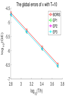
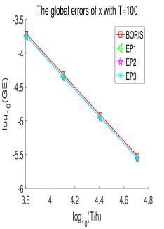
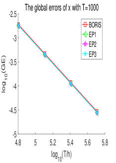
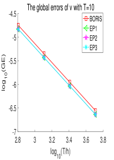
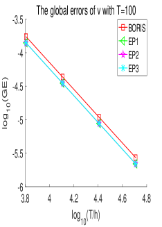
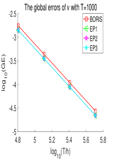
Figure 1: The logarithm of the global error against the logarithm of T/h.

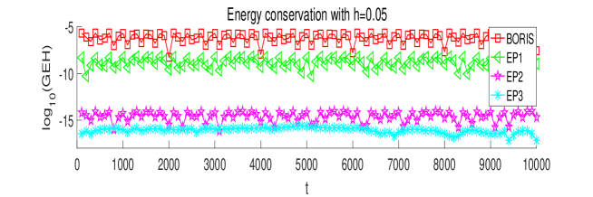
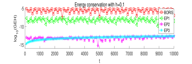
Figure 2: The logarithm of the error of energy against t.

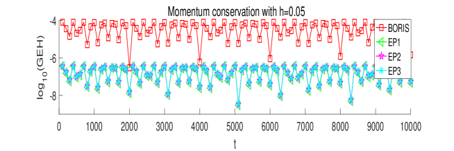
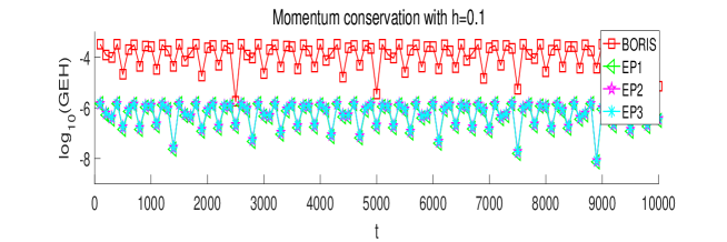
Figure 3: The logarithm of the error of momentum against t.

6 Conclusion

In this paper, the energy-preserving methods for solving charged-particle dynamics (1) were presented and studied. We analyzed and discussed its algebraic order and symmetry. Moreover, it was shown that our method can exactly preserve the energy of the charged-particle dynamics. We also proved that the momentum is nearly conserved along the novel methods over long times. A numerical experiment was performed and it was shown that our method is more effective and it can preserve the energy and momentum better than the Boris method.

References

- [1] V. I. Arnold, V. V. Kozlov, A. I. Neishtadt, Mathematical Aspects of Classical and Celestial Mechanics, Springer, Berlin, 1997
- [2] J. P. Boris, Relativistic plasma simulation-optimization of a hybird code, Proceeding of Fourth Conference on Numerical Simulations of Plasmas, pages 3-67. November 1970
- [3] H. Betsch, P. Steinmann, Inherently energy conserving time finite elements for classical mechanics, J. Comput. Phys., 160 (2000) 88-116.
- [4] L. Brugnano, F. Iavernaro, D. Trigiante, Hamiltonan Boundary Value Methods (Energy Preserving Discrete Line Integral Methods), J. Numer. Anal. Ind. Appl. Math. 5 (2010) 13-17.
- [5] L. Brugnano, F. Iavernaro, D. Trigiante, Energy- and quadratic invariants-preserving integrators based upon Gauss-Collocation formulae, SIAM J. Numer. Anal., 50 (2012) 2897-2916.
- [6] J. R. Cary, A. J. Brizard, Hamiltonian theory of guiding-center motion, Rev. Moder. Phys. 81 (2009) 693-738
- [7] D. Cohen, E. Hairer, Linear energy-preserving integrators for Possion systems, BIT, 51(2011)91-101.
- [8] E. Celledoni, B. Owren, Y. Sun, The minimal stage, energy preserving Runge-Kutta method for polynomial Hamiltonian systems is the averaged vector field method, Math. Comp., 83 (2014) 1689-1700.
- [9] J. B. Chen, M. Z. Qin, Multisympletic Fourier pseudospectral method for the nonlinear equation, Electron. Trans. Numer. Anal., 12 (2001) 193-204.
- [10] C. L. Ellison, J. W. Burby, and H. Qin, Comment on ”Symplectic integration of mag-netic systems”: A proof that the Boris algorithm is not variational. J. Comput. Phys., 301: 489C493, 2015.
- [11] E.Faou, E.Hairer, T.-L. Pham, Energy conservation with non-symplectic methods: examples and counter-examples, BIT 44 (2004) 699-709.
- [12] Gonzalez, O.: Time integration and discrete Hamiltonian systems. J. Nonlinear Sci. 6, 449-467(1996).
- [13] E. Hairer, Energy-preserving variant of collocation methods, J. Numer. Anal. Ind. Appl. Math. 5(2010) 73-84.
- [14] E. Hairer, C. Lubich, Energy behaviour of the Boris method for charged-particle dynamics. To appear in BIT, (2018)
- [15] E. Hairer, C. Lubich, Symmetric multistep methods for charged-particle dynamics, SMAI J. Comput. Math. 3 (2017) 205-218
- [16] E. Hairer, C. Lubich, G. Wanner, Geometric Numerical Integration: Structure-Preserving Algorithms for Ordinary Differential Equations, 2nd edn. Springer-Verlag, Berlin, Heidelberg, 2006.
- [17] Y. He, Y. Sun, J. Liu, H. Qin, Volume-preserving algorithms for charged particle dynamics, J. Comput. Phys. 281 (2015) 135-147
- [18] Y. W. Li, X. Wu, Functionally fitted energy-preserving methods for solving oscillatory nonlinear Hamiltonian systems, SIAM J. Numer. Anal., 54 (2016) 2036-2059.
- [19] Y. W. Li, X. Wu, Exponential integrators preserving first integrals or Lyapunov functions for conservative or dissipative systems, SIAM J. Sci. Comput. 38 (2016) 1876-1895.
- [20] T. Li, B. Wang, Explicit symplectic exponential integrators for charged-particle dynamics in a strong and constant magnetic field, (2018) arXiv:1810.06038
- [21] Y. Miyatake, An energy-preserving exponentially-fitted continuous stage Runge-Kutta method for Hamiltonian systems, BIT, 54 (2014) 777-799
- [22] Y. Miyatake, A derivation of energy-preserving exponentially-fitted integrators for poisson systems, Comput. Phys. Comm., 187 (2015) 156-161.
- [23] R. I. McLachlan, G. R. W. Quispel, Discrete gradient methods have an energy conservation law, Disc. Contin. Dyn, Syst., 34 (2014) 1099-1104.
- [24] R. I. McLachlan, G. R. W. Quispel, N.Robidoux, Geometric integration using discrete gradients, Philos. Trans. R. Soc. Lond. A 357 (1999) 1021-1045.
- [25] G. R. W. Quispel, D. I. McLaren, A new class of energy-preserving numerical integration methods, J. Phys. A, 41 (045206) (2008)7pp.
- [26] H. Qin, S. Zhang, J. Xiao, J. Liu, Y. Sun, W. M. Tang, Why is Boris algorithm so good? Physics of Plasmas, 20 (2013) 084503
- [27] M. Tao, Explicit high-order symplectic integrators for charged particles in general electromagnetic fileds, J. Comput. Phys. 327 (2016) 245-251
- [28] B. Wang, A. Iserles, X. Wu, Arbitrary-order trigonometric Fourier collocation methods for multi-frequency oscillatory systems, Found. Comput. Math. 16 (2016) 151-181
- [29] B. Wang, X. Wu, A new high precision energy-preserving integrator for system of oscillatory second-order differential equations, Phys. Lett. A, 376 (2012) 1185-1190.
- [30] B. Wang, X. Wu, The formulation and analysis of energy-preserving schemes for solving high-dimensional nonlinear Klein-Gordon equations, IMA J. Numer. Anal., in press, doi 10. 1093/imanum/dry047.
- [31] B. Wang, X. Wu, F. Meng, Trigonometric collocation methods based on Lagrange basis polynomials for multi-frequency oscillatory second-order differential equations, J. Comput. Appl. Math. 313 (2017) 185-201
- [32] X. Wu, B. Wang, Recent Developments in Structure-Preserving Algorithms for Oscillatory Differential Equations, Springer Nature Singapore Pte Ltd, 2018.
- [33] R. Zhang, H. Qin, Y. Tang, J. Liu, Y. He, J. Xiao, Explicit symplectic algorithms based on generating functions for charged particle dynamics, Phys. Revi. E 94 (2016) 013205