Triangle Extension: Efficient Localizability Detection in Wireless Sensor Networks

Abstract

Determining whether nodes can be localized, called localizability detection, is essential for wireless sensor networks (WSNs). This step is required for localizing nodes, achieving low-cost deployments, and identifying prerequisites in location-based applications. Centralized graph algorithms are inapplicable to a resource-limited WSN because of their high computation and communication costs, whereas distributed approaches may miss a large number of theoretically localizable nodes in a resource-limited WSN. In this paper, we propose an efficient and effective distributed approach in order to address this problem. Furthermore, we prove the correctness of our algorithm and analyze the reasons our algorithm can find more localizable nodes while requiring fewer known location nodes than existing algorithms, under the same network configurations. The time complexity of our algorithm is linear with respect to the number of nodes in a network. We conduct both simulations and real-world WSN experiments to evaluate our algorithm under various network settings. The results show that our algorithm significantly outperforms the existing algorithms in terms of both the latency and the accuracy of localizability detection.

1 Introduction

In wireless sensor networks (WSNs), owing to the high hardware and/or energy cost and indoor blindness of GPS components, localization algorithms are often required [1], [16], [19], [17], [25]. Such algorithms employ beacons, which are special nodes of known locations, to determine the unknown locations of the other nodes in a WSN [4], [20], [23]. An essential problem in localization algorithms is to detect whether a WSN or a node in the WSN is localizable [26]. For instance, most localization algorithms can only localize a relatively small percentage of nodes in a WSN, especially in sparsely deployed WSNs. A localizability detection algorithm can help such localization algorithms avoid non-stopping failures or incorrect localization answers. Localizability information also gives guidelines or identifies prerequisites to location-related applications, e.g., tracking and event detection. Finally, node localizability information is helpful for many mechanisms of WSNs, such as topology control, sensing area adaptation, and geographic routing.

The determination of whether a network is localizable is known as the network localizability problem, and the detection of whether a node is localizable is called the node localizability problem. The network localizability problem is formulated as follows [26]. A WSN is modeled as a connected graph: $G=(V,E)$, in which $i$ and $j$ are nodes and $(i,j)$ are the link between them ($i$, $j\in V$, $(i,j)\in E$). In $G$, the distance between $i$ and $j$, denoted as $d_{(i,j)}$, is known or can be measured, for example by using distance measuring methods [7], [8], [9] . The location of a node $i$, denoted as $p_{i}$, is known (beacon) or unknown (non-beacon). A graph $G$ with a constraint set $C$, e.g., a set that specifies the locations of the beacon nodes, is localizable when the following holds: For each node $i$ in $G$, there is a unique $p_{i}$, such that $d_{(i,j)}=distance(p_{i},p_{j})$ for all $(i,j)\in E$ and the constraint set $C$ is satisfied. Given such definitions, researchers have found a close relationship between the network localizability problem and the graph rigidity problem[6], [5], [10], [12], [13], [11]. A rigid graph has a finite number of frameworks with which it can be realized [13].

Although the graph rigidity testing algorithms are theoretically sound, such algorithms are not applicable to WSNs, as they only output false in most real-world WSNs[26]. Considering the realistic issues, researchers explore the node localizability problem instead of the network localizability problem. The following is an example of localizability testing, for node 1 in Fig.1. There are four nodes and nodes 2, 3, and 4 are beacons in Fig.1. Note that in Fig.1 and other network figures throughout this paper, an edge between two nodes indicates that the distance between the two nodes is known and fixed. As can be seen in Fig.1, for node 1, there are two possible locations that each satisfies these constraints. Each possible location of node 1 may have a possible network framework. Fig.1 shows two frameworks for the network. In conclusion, node 1 is not localizable.

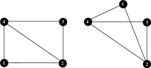
Figure 1: Two different frameworks of a network

Node localizability differs significantly from network localizability. The approach of simply partitioning a graph to a set of sub-graphs and detecting the localizability of the sub-graphs does not work for determining node localizability, as a partition may remove some constraints of the original network [26]. The problem is even more difficult when it is required to test the node localizability in a distributed way. A centralized approach may exhaust the energy of each node early in the process, as a packet of a source node usually needs to be forwarded many hops before it arrives at the center for processing. This problem is so difficult that no distributed solution has yet been found that can identify all theoretically localizable nodes.

In this paper, we propose an efficient and effective distributed algorithm to address the node localizability problem. Specifically, our algorithm employs a new method to extend each graph. In a graph, the extension of our algorithm starts from a sub-graph having only two beacon nodes and continues until the sub-graph reaches another beacon. Then, our algorithm determines whether the extended graph can be localized, according to graph rigidity theory. In particular, this paper makes the following contributions: (1) The proposed graph extension method is theoretically proved to be able to find localizable nodes with fewer beacons than the existing methods do. (2) The complexity of the distributed algorithm is shown to be linear to the number of nodes in a WSN. (3) Because of its low resource requirements, the algorithm is shown to be applicable to a sparsely deployed WSN. To our knowledge, the algorithm proposed in this paper is currently the best solution to the node localizability problem.

2 Preliminaries

2.1 Graph Rigidity

A rigid graph is a connected graph that has a finite number of frameworks [13]. Furthermore, if a graph has a unique framework, it is called globally rigid [10]. The graph shown in Fig.2(a) is rigid, as the graph has two and only two different frameworks in a 2-dimension($2D$) plane. In contrast, the graph shown in Fig.2(b) has an infinite number of frameworks; this is called a flexible graph. The graph in Fig.2(c) is globally rigid as it has only one framework. In the graphs, an edge between two nodes indicates that the distance between the two nodes is known.

(a)

(b)

(c)

Figure 2: Graphs: (a) rigid, (b) flexible, and (c) globally rigid

Suppose a graph $G$ satisfies the following two conditions: (1) it is globally rigid, (2) it contains three or more beacons that are non-collinear (i.e., they are not on the same line). Then, all the nodes in $G$ can be identified as localizable. Hence, the key issue for detecting localizability of a network is the detection of global rigidity.

2.2 Global Rigidity

We first review Hendrickson’s Lemma for the principle of detecting global rigidity. In Hendrickson’s Lemma, a skeletal sub-graph of $G$ contains all the vertexes of $G$. Then, we go on to the M-circuit [10], to learn how to construct a globally rigid graph. The notation is listed in Table I.

Hendrickson’s Lemma [10]: A graph is globally rigid if it is 3-connected and has a skeletal sub-graph that is a M-circuit.

Definition of M-circuit [10]: Graph $G$ is called an M-circuit if it satisfies the following two conditions:
(1) $|E_{G}|=2|V_{G}|-2$;
(2) for each $X\subseteq V_{G}$ with $2\leq|X|\leq|V_{G}|-1$, $|E[X]|\leq 2|X|-3$.

TABLE I: Notation in this paper

Notation	Description
G	An undirected and connected graph
$V_{G}$	Vertex set of graph $G$
$E_{G}$	Edge set of graph $G$
$|V|$	The number of nodes in $V$
$G[X]$	A sub-graph of $G$ induced by $X$; $X\subseteq V_{G}$
$E[X]$	The edge set of $G[X]$
$|E[X]|$	The number of edges in $G[X]$
$L_{x}$	The level of node $x$

According to Laman’s Lemma [13], a rigid graph can also be further broken down to a minimally rigid graph. Laman proved that every rigid graph $G$ has a skeletal sub-graph $G^{\prime}$ that is minimally rigid. Hence, each rigid graph can be reduced to a minimally rigid sub-graph by removing certain edges.

Laman’s Lemma[13]: A graph $G$ is minimally rigid if and only if $|E_{G}|=2|V_{G}|-3$ and for each $X\subset V_{G}$ with $2\leq|X|\leq|V_{G}|-1$, $|E[X]|\leq 2|X|-3$.

3 Related Work

A series of methods have been proposed to determine the rigidity of a graph [2], [12]. However, as most of these methods are centralized, they are not suitable for a real world WSN. A centralized algorithm needs the global information of the network topology to construct the adjacency matrix. However, because of the memory limit restriction on a node, it is unrealistic for each node to maintain the global topology information in a WSN, especially a large-scale WSN.

Yang and Liu previously proposed a theoretical approach for the detection of localizable nodes, called RR3P [26]. According to RR3P, a node in the network is localizable if the following two conditions hold: (1) the node belongs to a redundantly rigid component, and (2) in this component there exist at least three vertex-disjoint paths connecting the node to three distinct beacons. RR3P is not very suitable for distributed algorithms, as finding a redundantly rigid component requires near-global topology information about a network.

The differences between RR3P and our approach can be summarized as follows: (1) We propose a realistic distributed algorithm to find the localizable nodes starting from pairs of beacons. (2) Our distributed algorithm is able to detect most of the localizable nodes without finding the redundantly rigid component which is the prerequisite in RR3P. (3) In our distributed algorithm, each node only uses the information from one-hop communication. In comparison, RR3P needs to detect the three vertex-disjoint paths, which usually span several hops.

Eren et al. proposed a distributed algorithm, the $trilateration~{}protocol$ (TP) [5], to mark the localizable nodes and calculate their locations in a network. The general idea of TP is that a node can be regarded as localizable, whenever the node can identify three or more localizable neighbors. This idea enables TP to be fully distributed. Hence, TP has been used by many applications , [21]. Eren recently proposed the concepts of indices to quantitatively measure the network graph rigidity [6]. Such concepts are also helpful to these applications.

However, TP may miss localizable nodes that are on a $geographical~{}gap$ or in a graph with $border~{}nodes$. Fig.3(a) is a graph with a geographical gap. The nodes without labels are detected to be localizable. Nodes $A$, $B$, and $C$ are theoretically localizable. However, none of the nodes among $A,B,C$ will be determined to be localizable by TP, because none of them has three or more localizable neighbors. In Fig.3(b), nodes $A$ and $B$ are border nodes. They can not be determined to be localizable by TP, either.

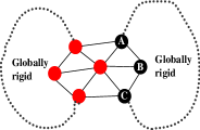
(a)Geographical gap

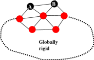
(b)Border nodes

Figure 3: Deficiency of trilateration protocol

To solve the problems of a geographical gap and of border nodes, Yang et al. proposed a new fully distributed approach for detecting localizable nodes, called $wheel~{}extension$ (WE) [27]. In a WSN running WE, each node tries to construct wheel graphs within its neighbors. During the extension process, each node only needs to check the constructed wheel graphs. If there are three or more nodes that are localizable in a wheel graph, WE marks all the other nodes in the wheel graph as localizable.

Nonetheless, there are often scenarios in which WE may not work well, either. For example, it may be the case that beacons are not present in any wheel graphs in a network. Another scenario is one in which a node cannot build a wheel graph, because of the lack of adequate network information for the node. As shown in Fig.4, none of the nodes in graph $G_{c}$ are in a wheel graph and there is no node that has three or more localizable neighbors. Therefore, neither TP nor WE can find any localizable node in graph $G_{c}$. However, as we will show later, all the nodes in a graph such as $G_{c}$ are localizable.

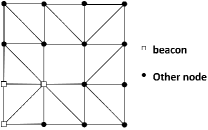
Figure 4: $G_{c}$, A globally rigid graph.

In contrast with WE and TP, our algorithm uses a new detection method, $triangle~{}extension$ (TE), to find the localizable nodes in a WSN. TE can start with far fewer beacons than the existing algorithms. Moreover, TE not only works well for a graph such as $G_{c}$ in Fig.4, but also avoids the problems shown in Fig.3.

4 Triangle Extension Theory

This section presents our theoretical approach to node localizability detection via global rigidity as follows: We define the concept of a branch and propose related lemmas. These concepts and lemmas enable us to construct a graph that is an M-circuit and globally rigid, starting from a branch.

4.1 Branch Concept

We introduce three concepts that will enable us to define a branch. The first is an operation called extension. The second is a special kind of extension: triangle extension. Triangle block is the third concept. A branch will then be constructed within a triangle block.

Extension: Given a graph $G$, an extension operation on $G$ is one that inserts a new vertex $v$ into $V_{G}$ and two edges $(v,r_{1}),(v,r_{2})$ ($r_{1},r_{2}\in V_{G}$) into $E_{G}$. Here, nodes $r_{1}$ and $r_{2}$ are said to be extended by node $v$. Nodes $r_{1}andr_{2}$ are called the parents of $v$ and $v$ is called a child of $r_{1}andr_{2}$. The ancestors of node $v$ are recursively defined as $v$’s parents ($r_{1}andr_{2}$) and the ancestors of $v$’s parents.

Lemma 1 gives the property of extensions. Its proof is in Appendix A. Following Lemma 1, when performing a series of extensions from a minimally rigid graph $K_{2}$, we can obtain a larger minimally rigid graph. $K_{2}$ is a complete graph of two nodes and is minimally rigid according to Laman’s Lemma [13]. Fig.5 shows the extensions from a $K_{2}$ graph(the leftmost graph with only $r_{1}$ and $r_{2}$). In this figure, the graph is extended by nodes $a$, $b$, $c$, $d$, and $e$, after five extension operations. The final resulting graph is still minimally rigid.

Lemma 1.

A graph $G_{1}$, generated from a series of extensions on a minimally rigid graph $G$, is also minimally rigid.

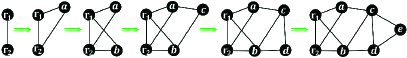
Figure 5: A series of extensions

Triangle Extension: A triangle extension operation is a sequence of extensions, the first of which starts from a $K_{2}$. As shown in Fig.5, the extension sequence launched by nodes {$a$, $b$, $c$} and that launched by nodes {$a$, $b$, $c$, $d$, $e$} are both triangle extensions, but the extension sequence of {$d$, $e$} is not a triangle extension, as it does not start from a $K_{2}$.

Triangle Block: A triangle block is a graph constructed from a $K_{2}$ graph by a triangle extension. The nodes in the original $K_{2}$ are called the roots of this triangle block. In a triangle block, a node $x$ has a level denoted as $L_{x}$. If $x$ is a root, $L_{x}$ = 0; otherwise, $L_{x}$ = 1 + max(the levels of $x$’s parents). The value of the level indicates the temporal order of the extension.

Branch: In a triangle block $T$, a branch of $T$ is a sub-graph of $T$ that is composed of a node $v$, the ancestors of $v$, and the edges between them. Node $v$ is called the leaf node and the branch is denoted using $B(v)$ to indicate that the leaf node is the end of the triangle extension. The roots $r_{1}$ and $r_{2}$ of $T$ are also the roots of $B(v)$. Fig.6 shows the four branches $B(c)$, $B(d)$, $B(e)$, and $B(f)$ of $T$.

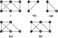
Figure 6: Example triangle block and its branches

A branch has two following properties. Property-1: A branch is minimally rigid. Property-2: Removing any single node from a branch will not cause the branch to become disconnected. Property-1 can be derived from Lemma 1 as a branch is extended from a $K_{2}$. Property-2 can be proved as follows: It is evident that removing the leaf or one of the roots will not break a branch into two separate sub-graphs. Given a non-root and non-leaf node $x$ in a branch, the number of edges connected to $x$ is at least 3. The reason is that node $x$ must have two parents and at least one child connected to itself in a branch. Hence, removing $x$ will not cause the branch to become disconnected. Property-2 holds.

Lemma 2.

Branch Lemma: In a branch $B(v)=(V_{B},E_{B})$, there is no set $X$ that satisfies all of the following three conditions.
(1) $X\subsetneqq V_{B}$, where $V_{B}$ is the vertices of $B(v)$.
(2) $X$ contains the two roots of $B(v)$ and $v$.
(3) $|E[X]|=2|X|-3$.

Proof.

In the scenario of $L_{v}=1$, i.e., node $v$ is at level 1, $B(v)$ only contains $v$ and the two roots, which are also the parents of $v$. It is evident that conditions (1) and (2) cannot be satisfied at the same time.

In the scenarios of $L_{v}\geq 2$, we prove Lemma 2 by contradiction: Suppose that there is a set $X$ satisfying all three conditions. Let $Y=V_{B}-X$.

When there is only a single node $y$ in $Y$, $y$ is neither a root nor the leaf node since they are in $X$. The number of edges connected to $y$ is at least three. Subsequently, as $|E[X]|=2|X|-3$, $|E[X\cup y]|\geq 2|X\cup y|-2$. On the other hand, since $B(v)$ is a minimally rigid graph (Branch Property-1), according to Laman’s Lemma, for each $X^{\prime}\subset V_{G}$ with $2\leq|X^{\prime}|\leq|V_{G}|-1$, $|E[X^{\prime}]|\leq 2|X^{\prime}|-3$. Let $X^{\prime}=X\cup y$; then $|E[X\cup y]|\leq 2|X\cup y|-3$ contradicts the previous deduction: $E[X\cup y]\geq 2|X\cup y|-2$.

When there is more than one node in $Y$, we proceed as follows: Let $ym$ be the node in $Y$ having the smallest level. As $ym$ has at least two parents in $X$, the number of edges connected to $ym$ is at least two. We move $ym$ from $Y$ to $X$ and obtain $|E[X]|\geq 2|X|-3$. Similarly, we can move each node with the smallest level from the remainder nodes in $Y$ to $X$ until there is only a single node in $Y$, denoted as $ym^{\prime}$. Then there are at least three edges connected to $ym^{\prime}$, since the parents of $ym^{\prime}$ and the children of $ym^{\prime}$ are all in $X$ now. After we move $ym^{\prime}$ into $X$, we have $|E[X]|\geq 2|X|-2$. This is in conflict with Laman’s lemma.

In summary, regardless of whether $L_{v}=1$ or $L_{v}\geq 2$, there is no $X$ that satisfies all of the three conditions. ∎

4.2 Globally Rigid Graph Construction Theorem

We now start to build a globally rigid graph from a branch. The steps are as follows: First, we deduce Lemma 3 to obtain a 3-connected graph from a branch. Then, we prove that the constructed graph is an M-circuit, according to Lemma 2 of the last subsection. As a result, the two necessary conditions for obtaining a global rigidity graph are met.

Lemma 3.

In a branch $B(v)$, the removal of two nodes $t_{1}$ and $t_{2}$, where $v\notin\{t_{1},t_{2}\}$ and there is at most one root in $\{t_{1},t_{2}\}$ divides $B(v)$ into at most two sub-graphs. If after the removal of $t_{1}$ and $t_{2}$, $B(v)$ is divided, the leaf node $v$ and the remaining root(s) are in different sub-graphs.

Proof.

As a branch is a 2-connected graph, the removal of a single node will not divide the branch into two separate sub-graphs. Then removing another node may divide the graph into at most two separate sub-graphs. Furthermore, the removal of two nodes cannot divide a branch of three nodes into two sub-graphs. The following are the three possible scenarios for $t_{1}$ and $t_{2}$.

(I) $\{t_{1},t_{2}\}$ does not contain any root. We consider a node $t$, $t\in\{t_{1},t_{2}\}$. As $t$ has two different parents and each ancestor of $t$ has two different parents, there are two different routes with no intersection from $t$’s two parents to the roots, $r_{1}$ and $r_{2}$. Similarly, the routes from $v$’s two parents to $r_{1},r_{2}$ have no intersection either. Fig.7(a) shows the branch. The three routes, those from $t$ to $v$, from $t$ to $r_{1}$, and from $t$ to $r_{2}$, only intersect at $t$. The dash-dotted lines in Fig.7 and other figures in this paper illustrate the edges between the roots or beacons (as their distances are known). Suppose $t_{1}=t$; then $t_{2}$ should be on the other route from $v$ to the roots. Otherwise, the removal of $t_{1}$ and $t_{2}$ does not divide $B(v)$. As such, if the removal of $t_{1}$ and $t_{2}$ causes $B(v)$ to be divided into two sub-graphs, the two disjoint routes from $v$ to $r_{1},r_{2}$ must have been cut off. Therefore, $v$ is in a different graph from that of the two roots.

(II) $t_{1}$(or $t_{2}$) is a root. For simplicity, let $t_{1}=r_{1}$. Then $t_{2}\notin\{r_{1},r_{2},v\}$, in which case $t$ has two disjoint routes to $r_{2}$ and $v$. These two routes do not contain $r_{1}$, as $r_{1}$ is a root. Hence, the removal of $t_{2}$ will not break these two disjoint routes to $r_{2}$ and $v$. In summary, there is no node $t_{2}$ that together with $r_{1}$ will divide the branch while keeping $r_{2}$ and $v$ in the same component.

(III) $\{t_{1},t_{2}\}=\{r_{1},r_{2}\}$; i.e., $t_{1}$ and $t_{2}$ are the two roots. In this scenario, $v$ has a path to all its ancestors left in $B(v)$. $B(v)$ can not be divided by removing $\{r_{1},r_{2}\}$. Therefore, $\{t_{1},t_{2}\}$ contains at most one of the roots.

From the above, node $v$ and the remaining root(s) are in different sub-graphs if $B(v)$ is broken into two sub-graphs after the removal of two nodes. ∎

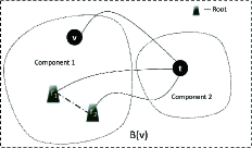
(a) Branch division

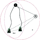
(b) Globally rigid graph construction

Figure 7: Branch and construction of globally rigid graph (dash-dotted lines: existing edges with fixed distances)

Using Lemma 3, the graph $G$ composed of $B(v)$, $q$, $(q,v),(q,r_{1}),(q,r_{2})$ such as that in Fig.7(b) can be proved to be 3-connected: First of all, if $q$ in $G$ is removed, then $G$ becomes $B(v)$, which is still a connected graph. Then, removing any two nodes of $B(v)$ divides $B(v)$ into at most two disconnected sub-graphs, as a branch is 2-connected. From Lemma 3, after the removal of two more nodes, if $B(v)$ is divided into two graphs, then $v$ and the roots must be in different graphs. Therefore, $G$ is 3-connected. If $G$ is further proved to be an M-circuit, then $G$ can be claimed as a globally rigid graph. Theorem 1 shows how to obtain an M-circuit.

Theorem 1.

Given a branch $B(v)$, where $B(v)=(V_{B},E_{B})$, if a graph $G$ is constructed by adding a new vertex $q$ into $V_{B}$ and three edges $(q,v),(q,r_{1}),(q,r_{2})$ into $E_{B}$, then $G$ is globally rigid.

Proof.

Consider a branch $B(v)$ and a graph $G$ obtained by adding node $q$, and edges $(q,v),(q,r_{1}),(q,r_{2})$ to $B(v)$. Using Lemma 3, as mentioned above, $G$ can be proved to be 3-connected. This 3-connected property leads to the following equations: $|E_{B}|=2|V_{B}|-3$, $|E_{G}|=|E_{B}|+3$ and $|V_{G}|=|V_{B}|+1$; and finally $|E_{G}|=2|V_{G}|-2$.

Given a node set $X$, $X\subseteq V_{B}$, if node $q\notin X$, then $|E[X]|\leq 2|X|-3$ since $B(v)$ is minimally rigid and $X$ is a subset of the nodes in $B(v)$. If $q\in X$, we prove by contradiction. We assume $|E[X]|\geq 2|X|-2$. Let $X^{\prime}=X-q$. As node $q$ has at most three edges connected to the nodes in $X$, we have $|E[X^{\prime}]|\geq 2|X^{\prime}|-3$ and $X^{\prime}\subsetneqq V_{B}$ after the removal. Because $X^{\prime}\subsetneqq V_{B}$ and $B(v)$ is minimally rigid, $|E[X^{\prime}]|>2|X^{\prime}|-3$ does not hold. From Lemma 2, $|E[X^{\prime}]|=2|X^{\prime}|-3$ is not possible, either. As a result, the assumption $|E[X]|\geq 2|X|-2$ does not hold and thus only $|E[X]|\leq 2|X|-3$ holds. Now that for each $X\subsetneqq V_{2}$ with $|X|\geq 2$, $|E[X]|\leq 2|X|-3$ holds, the 3-connected graph $G$ can be concluded to be an M-circuit. Therefore, $G$ is globally rigid. ∎

5 Distributed Localizability Detection Using Triangle Extension

In this section, we propose a distributed approach to localizability detection through triangle extensions. Fig.8 provides an example to illustrate this idea. In Fig.8, there are two nodes in the initial stage, $r_{1}$ and $r_{2}$, which constitute a $K_{2}$ graph. In the first step, by triangle extension, $v_{1}$ extends $r_{1}$ and $r_{2}$ to form the branch $B(v_{1})$. Then, $v_{2}$ is added as the leaf node to form the branch $B(v_{2})$. Finally, the node $q$, which has edges to $r_{1}$ and $r_{2}$, is found to be a neighbor of $v_{2}$. According to Theorem 1, the graph $G$, which contains both $q$ and $B(v_{2})$, is globally rigid. Supposing that the locations of nodes $q$, $r_{1}$ and $r_{2}$ are known and the three nodes are not on the same line, all of the nodes in Branch $B(q)$ can be determined to be localizable.

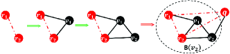
Figure 8: A complete example of branch construction and global rigidity determination

Our approach proceeds in two phases: the extension phase and the detection phase. In the detection phase, a node determines its localizability $state$ according to the received messages. The nodes in a WSN may be in any of the following three states: flexible, rigid and localizable. The state of a beacon is initialized as localizable since its location is known and fixed.

The details of the two phases are as follows. In the extension phase, the states of beacons are first labeled as localizable, and those of the other nodes are labeled as flexible. Then, a pair of beacons triggers the extension operations on their neighbor nodes. In turn, certain neighbor nodes will be added to form triangle blocks. These newly added nodes change their states to rigid and inform their neighbors. In the detection phase, when a node $v$ changes its state from flexible to rigid, it checks whether the following two conditions are satisfied; if so, then all of the nodes in $B(v)$ can be determined to be localizable.
(1) $v$ has a localizable neighbor $q$ that is not an ancestor of $v$ in $B(v)$.
(2) Locations of $q$ and the roots of the branch are not collinear (not on the same line).

We now formulate the initial version of the distributed localizability detection algorithm using the triangle extension, denoted as ITE. ITE has two phases: extension and detection as shown in Procedure 1 and Procedure 2, respectively. In Procedure 1, initially a node broadcasts messages that contain its unique ID, its current state and its location (if known). A node in the flexible state performs extensions after measuring distances to its neighbors: (1) It chooses a pair of neighbors as its parents and updates its state to rigid (Lines 11–20). (2) It broadcasts the state information to its neighbors (Lines 21–22). In Procedure 1, the sets $P$ and $B$ denote the parent set and branch set on the node.

Procedure 1 Extension Phase

1:  type b: {state, parents{NULL, NULL},roots{NULL, NULL} } // b: branch tuple

2:  type p: {id, b} // p: a candidate of parents for this node

3:  $P\leftarrow\phi$ //$P$: set of $p_{i}$, $i=1,2,3,...$

4:  $B\leftarrow\phi$ //$B$: set of $b_{i}$, $i=1,2,3,...$

5:  Initialization($this.id,P,B$) // the states of beacons are set as localizable

6:  if ReceivedMessagesFromNeighbors($p_{i}$) then

7:      $P$.Add($p_{i}$)

8:      for $p_{j}$ in $P$ do

9:         if $p_{i}=p_{j}$ then

10:             continue

11:         if $p_{i}$ is $beacon$ then

12:             if $p_{j}$ is $beacon$ then

13:                $B$.Add(new b($state\leftarrow rigid,parents\leftarrow\{p_{i},p_{j}\},roots\leftarrow\{p_{i},p_{j}\}$))

14:             else if $p_{i}\in p_{j}.roots$ then

15:                $B$.Add(new b($state=rigid,parents\leftarrow\{p_{i},p_{j}\},roots\leftarrow p_{j}.roots$))

16:         else

17:             if $p_{j}.state$ = $localizable$ and $p_{j}\in p_{i}.roots$ then

18:                $B$.Add(new b($state\leftarrow rigid,parents\leftarrow\{p_{i},p_{j}\},roots\leftarrow p_{i}.roots$))

19:             else if $p_{i}.roots$ equals $p_{j}.roots$ then

20:                $B$.Add(new b($state\leftarrow rigid,parents\leftarrow\{p_{i},p_{j}\},roots\leftarrow p_{i}.roots$))

21:  for $b_{i}$ in $B$ do

22:      Broadcast(new p($this.id$, $b_{i}$))

The nodes in Fig.8 are taken as an example to show how the triangle extension and detection are launched. Initially, every node runs Procedure 1. Node $v_{1}$ finds that its two parents $r_{1}$ and $r_{2}$ are two beacons when it receives the messages from these two parents (Line 6). It then adds them to form its branch $B(v_{1})$, as shown in Lines 11–13. This step starts a triangle extension. Next, $v_{1}$ updates its state to rigid and integrates this new state and branch information into a parent candidate, $p$. Finally, $v_{1}$ broadcasts $p$ to its neighbors (Line 22). $v_{2}$ receives $p$ and adds $v_{1}$ and $r_{2}$ to construct a new branch $B(v_{2})$ (Lines 14–15). The triangle extension comes to $v_{2}$. Procedure 2 on a node detects whether there is an extra localizable neighbor that is non-collinear with the two roots of the branch of this node. If so, the node marks itself as localizable and broadcasts this news to its neighbors.

Procedure 2 Detection Phase

1:  if ReceivedMessagesFromNeighbors($p_{n}$) then

2:      if $p_{n}$ is a beacon then

3:         for $b_{i}$ in $B$ do

4:             if $p_{n}\notin b_{i}.roots$ and non-collinear($b_{i}.roots$, $p_{n}$) then

5:                $b_{i}.state\leftarrow localizable$

6:      else if $p_{n}.state=localizable$ and ($this.id=p_{n}.parents[0].id$ or $this.id=p_{n}.parents[1].id$) then

7:         for $b_{i}$ in $B$ do

8:             if $b_{i}.roots$ equals $p_{n}.roots$ then

9:                $b_{i}.state\leftarrow localizable$

10:  for $b_{i}$ in $B$ do

11:      if $b_{i}.state=localizable$ then

12:         Broadcast((new p($this.id,b_{i}$))

We use the previous figure, Fig.8, to show how Procedure 2 works. As given in Procedure 1, node $q$ finally receives the branch information from its parents. Since node $q$ is a beacon, it notifies its localizability state back to its neighbors. After $v_{2}$ receives this information from $q$, it proceeds Lines 2-5, and notifies all its neighbors that the nodes on the branch of $v_{2}$ are all localizable.

In Algorithm ITE, a node finds two neighbor nodes and extends them if these two neighbors are in the same triangle block as itself. The node can find out whether it shares the same triangle block with the two neighbors, by comparing the roots of the neighbors with itself. The two neighbors are then marked as the possible parents of this node. Each node maintains a set of possible parents and a set of branches. The extension phase on each node covers all pairs of neighbors in the branch set. In the detection phase, a traversal of set $B$ is performed to inform all neighbors. Therefore, the time complexity of ITE is O($m^{2}$), where $m$ is the number of neighbors of a node has.

We also analyze the space complexity of the two sets $P$ and $B$ due to the space limit of a sensor node. The number of neighbors of a node in a sparse network is usually relatively small, on the order of tens. Therefore, a single resource-modest sensor node can maintain the two sets. Take node $d$ in the WSN of Fig.9(a) as an example. Node $d$ only needs to put four nodes, $r_{2}$, $a$, $b$, and $c$, into its set $P$. In Fig.9(a), the ancestors’ topologies are transparent to node $d$, and thus there are only six different branches in its neighborhood. In general, within a branch any pair of neighbors of a node can be the node’s parents and any pair of beacons can be the roots. Hence, there are at most $\binom{m}{2}*\binom{k}{2}$ different branches for a node, supposing there are $m$ neighbors of a node and $k$ beacons on average ($m\geq 2$, $k\geq 2$). Node $d$ can construct six different branches and these are all listed in Fig.9(b) .

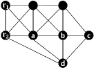
(a) Working scenario for TP and TE

(b) The six branches on node $d$

Figure 9: Space complexity analysis example

As most sensor nodes are highly resource-limited, it is inefficient for a node to maintain a set of all its branches in practice. Hence, ITE is not applicable to large-scale networks. A naive method is to limit the size of the branch set, but it is difficult to locally choose the best branch for a node itself. The best branch can help the node to detect the most localizable nodes.

To address this resource limitation problem, we next propose an advanced extension operation, called directed-extension, as follows. The extension operation in ITE is not directed. For instance, the undirected extension of ITE can add a new node $v$ in $G$ and two edges ($v$,$v_{1}$), ($v$,$v_{2}$) to form $B(v)$, as long as $v_{1},v_{2}\in V_{G}$. In directed-extension, $v$’s parents $v_{1}$ and $v_{2}$ should conform to the following additional rule: $v_{1}$ should be a parent of $v_{2}$ or $v_{2}$ a parent of $v_{1}$ if they are not the two roots. Fig.10 shows an example: when $b$ is to be added to form $B(b)$, its parent $a$ and another parent $r_{2}$ conform to the rule, as $r_{2}$ is a parent of $a$. Furthermore, in directed-extension, once a node changes its state to rigid, it will no longer accept any other nodes as its parents. This way, the extension will follow only one direction.

Directed-extension holds the property of minimally rigidity, since the new branch set of node $v$ is a subset of the branch set in the original (undirected version) extension. Because the directed-extension approach limits the extension possibilities, the set $B$ can be reduced significantly. In Fig.10, a node sequence such as ($a,b,c,d,e,f$) is called a directed triangle extension path and this extension path specifies a unique branch.

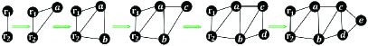
Figure 10: Directed-extension

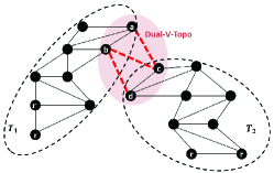
Figure 11: Triangle blocks meeting

Nonetheless, directed-extension has an early-stop problem. Suppose that in a WSN as shown in Fig.11 there are two pairs of beacons ( each root is denoted as $r$ for simplicity). Each pair of beacons can create a triangle block, denoted as $T_{1}$ and $T_{2}$ respectively. After a series of extensions, $T_{1}$ might overlap $T_{2}$ as shown in the shaded area of Fig.11. The special topology in the overlapping area of $T_{1}$ and $T_{2}$ is named as Dual-V-Topo. The Dual-V-Topo is composed of four nodes and five edges, in which two of the nodes have three edges each. As the directed-extension on a node stops when the node changes its state to rigid, the nodes $a$, $b$, $c$ and $d$ perform no further extension operations. As a result, since there are no more than three non-collinear beacons in each block, neither graph $T_{1}$ nor graph $T_{2}$ can be determined to be localizable. However, the two blocks can actually be determined to be localizable by the original undirected triangle extension approach, ITE.

To address this early-stop problem, we modify the detection phase to dual-v-detection. A node in a branch may launch dual-v-detection when it finds rigid neighbors in a triangle block other than its own. For example, in the network of Fig.11, the extension from $b$ to $a$ and the extension from $d$ to $c$ finish at the same time. Next, node $c$ learns that it can access rigid neighbors $a$ and $b$, both of which belong to a different triangle block. Node $c$ will launch the dual-v-detection procedure to test whether node $d$ can access $a$ or $b$. $T_{1}$ and $T_{2}$ can be connected by the three edges $(a,c)$, $(b,c)$, and $(b,d)$ when node $c$ confirms that node $d$ can access $a$ or $b$. The two connected triangle blocks can be determined localizable. This procedure for determining the localizability of $T_{1}$ and $T_{2}$ is called dual-v-detection. Combining the directed extension (Procedure 3), and the dual-v-detection procedure (Procedure 4), we propose the final version of the localizability detection algorithm via triangle extension, denoted as TE.

Procedure 3 TE-Extension Phase

1:  type $b$: {state, parents{NULL, NULL},roots{NULL, NULL} } // b: branch tuple

2:  type $p$: {$id$, $b$} // p: a candidate of parents for this node

3:  $P\leftarrow\phi$ // $P$: set of $p_{i}$

4:  Initialization($myp$) //$myp$, $p_{i}$ and $p_{j}$ represent instances of type p

5:  if ReceivedMessagesFromNeighbors($p_{i}$) then

6:      $P$.Add($p_{i}$)

7:      for $p_{j}$ in $P$ do

8:         if $p_{i}.id=p_{j}.id$ then

9:             continue

10:         if $p_{i}.state$ = $beacon$ then

11:             if $p_{j}.state$ = $beacon$ then

12:                $myp.state\leftarrow rigid$; $myp.parents\leftarrow\{p_{i},p_{j}\}$; $myp.roots\leftarrow\{p_{i},p_{j}\}$

13:                break

14:             else if $p_{i}\in p_{j}.parents$ then

15:                $myp.state\leftarrow rigid$; $myp.parents\leftarrow\{p_{i},p_{j}\}$; $myp.roots\leftarrow p_{j}.roots$

16:         else

17:             if $p_{j}.state$ = $localizable$ and $p_{j}\in p_{i}.parents$ then

18:                $myp.state\leftarrow rigid$; $myp.parents\leftarrow\{p_{i},p_{j}\}$; $myp.roots\leftarrow p_{i}.roots$

19:                break

20:             else if $p_{i}\in p_{j}.parents$ or $p_{j}\in p_{i}.parents$ then

21:                $myp.state\leftarrow rigid$; $myp.parents\leftarrow\{p_{i},p_{j}\}$; $myp.roots\leftarrow p_{i}.roots$

22:                break

23:      if $myp.state\neq flexible$ then

24:         Broadcast($myp$)

25:         break

Procedure 4 TE-Detection Phase

1:  if ReceivedMessagesFromNeighbors($p_{n}$) then

2:      $P$.Add($p_{n}$) //$p_{n},p_{i}$: type p

3:      if $p_{n}.state=beacon$ then

4:         if $p_{n}\notin myp.roots$ and non-collinear($myp.roots$, $n$) then

5:             $myp.state\leftarrow localizable$

6:      else if $p_{n}.state=localizable$ and $myp\in p_{n}.parents$ then

7:         $myp.state\leftarrow localizable$

8:      else if $p_{n}.roots\neq myp.roots$ and non-collinear($n.roots$, $myp.roots$) then

9:         //Dual-V-Topo detection

10:         for $p_{i}$ in $P$ do

11:             //find the child and parent in $P$, check parents’ neighbors

12:             if $p_{n}\in p_{i}.parents$ or $p_{i}\in p_{n}.parents$ then

13:                if $p_{n}\in parents.P$ or $p_{i}\in parents.P$ then

14:                    $myp.state\leftarrow localizable$

15:                    break

16:  if $myp.state=localizable$ then

17:      Broadcast($myp$)

In TE, a node in a WSN broadcasts at most twice, once for the state transition from the flexible state to the rigid state and the other time for the notification of the success of localizability detection. In a WSN, the first traversal launched by two beacons creates several minimally rigid triangle blocks. The second traversal from the third beacon to the roots of a certain branch $B(v)$ in these blocks informs all the nodes in $B(v)$ that they are localizable. Hence, the time complexity of TE is $O(n)$, where $n$ is the number of nodes in the WSN. In TE, each node keeps the information about the neighboring beacon and rigid nodes. Such information takes $O(m)$ space, where $m$ is the number of neighbors. To find the pair of connected neighbors, TE searches every pair of neighbors on each node. Hence, TE has a time complexity of $O(m^{2})$, which is acceptable since $m$ is usually small, especially in a sparse network.

The following discusses the advantages of TE over the other two previous approaches, TP and WE. The network scenarios that TP, WE, and TE work with are shown in Fig.12(a),(b). TE additionally works in the network scenario of Fig.12(c), where TP and WE cannot. In Fig.12, $r_{1}$, $r_{2}$, and $q$ are beacons and their distances are known before the algorithms run. Their distances are denoted using the dash-dotted lines. As shown in Fig.12(a), TP requires the three beacons to be the neighbors of a single node so that TP can measure the distances between node $v$ and the beacons. TE works in this scenario by a triangle extension. As shown in Fig.12(b), WE requires three beacons within a $wheel$. The dashed arrows in Fig.12(b) show the sequence of extensions by TE. As the extensions from $r_{1}$ and $r_{2}$ finally come to $q$, the nodes can be determined to be localizable by TE.

Fig.12(c) presents a common network in which many nodes such as $v_{3}$–$v_{6}$ are not neighbors of beacons. Nonetheless, they can extend from beacons by a sequence of extensions, as shown by the numbers 1 to 7 in Fig.12(c). In this figure, when $v_{7}$ performs the last extension(No. 7), $v_{7}$ determines that $B(v_{7})$ is localizable, since its neighbor $q$ is a beacon and the three beacons, $q$, $r_{1}$, and $r_{2}$ constitute a triangle. $v_{7}$ then broadcasts back to its parents, $v_{5}$ and $v_{6}$, that the branch $B(v_{7})$ is localizable. Similarly, $v_{4}$, $v_{3}$, and $v_{1}$ are notified by their children that the branch is localizable. The localizability of node $v_{2}$ cannot be determined, however, because it is not in $B(v_{7})$ but in $B(v_{2})$.

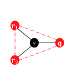
(a) Scenario of TP and TE

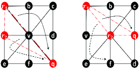
(b) Scenario of WE and TE

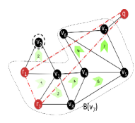
(c) Additional scenario of TE

Figure 12: Comparison of TP, WE and TE

6 Evaluation

6.1 Simulation

We first used TOSSIM [14] to run the three localizability detection algorithms: TE (ours), WE [27] and TP [5]. TOSSIM is a scalable WSN simulator that can simulate the behaviors of application programs in a WSN with hundreds of nodes[14]. The application programs tested on TOSSIM can be directly executed on actual sensor nodes. Table II shows the simulation setup, including the network and beacon deployment parameters. The deployment area was partitioned evenly into 20 $\times$ 20 cells and each node was placed into a random cell. The cell has a side length of $D_{0}\times N$, where $D_{0}$ is set as the standard unit for node distance and $N$ the network density parameter. The average range for reliable communication of simulated nodes is within $6D_{0}$. Therefore, we set the maximum value for $N$ to 5.8, to allow the neighboring sensor nodes to communicate. A smaller $N$ value leads to a higher network density in terms of the number of nodes deployed in a unit area.

TABLE II: Simulation setup

Parameter	Definition	Value
$S$	Scale: number of nodes in a WSN	$S=400$
$C$	Num of correctly detected localizable nodes	$0\leq C\leq S$
$D_{0}$	Unit of distance between nodes	10 m
$B$	Beacon density	$0.01\leq B\leq 0.2$
$N$	Network density	$2.0\leq N\leq 5.8$
$L$	Localizability detection accuracy: $\frac{C}{S}$	$0.0\leq L\leq 1.0$

The simulations were run under different beacon and node densities to reveal how these factors affect the node localizability detection in WSNs. A beacon continued broadcasting its location periodically in each simulation. The assumption is that the locations of beacons in the simulations and experiments are accurately set and thus will not introduce location biases.

To obtain a comprehensive view of the performance of the algorithms under evaluation, we performed a series of simulations with two parameter sets with (1) $B=0.04$ and (2) $B=0.1$. The network density parameters in the two sets are $N=2.4$, $N=3.2$, and $N=4.2$. These two parameter sets specify six WSNs, from a low beacon density and network density to a high beacon density and network density. We ran each algorithm 30 times on TOSSIM under the two parameter sets. Fig.13 shows $L$, which is the average percentage of detected localizable nodes over the total number of nodes in the WSN, for the three algorithms. The range line on the bar for an algorithm shows the upper and lower bounds of $L$ for that algorithm. The results show that TE performed the best on average. Furthermore, TE is stable as the upper and lower bounds of $L$ for TE are close together. The bounds actually show the localizability detection probability distribution of an algorithm.

TE performed especially well when the network and beacons were sparse. Sparse beacons are typical scenarios in WSN applications, since it is often infeasible to deploy a network with up to 10% beacons and short node distances. In addition, a high network density is not realistic, either. The parameter value of $N=2.4$ might result in about 50 neighbors for an internal node. This large number of neighbors is good for localizability detection but it is not efficient, as there may be heavy radio interference and the node energy will be exhausted early on.

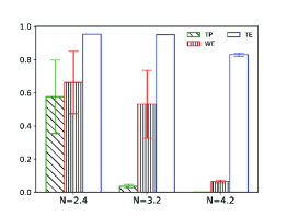
(a) B = 0.04: low beacon density

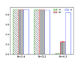
(b) B = 0.1: high beacon density

Figure 13: Percentages of localizable nodes under different beacon and network densities

Fig.14 records the values of $L$ while $B$ and $N$ are gradually changed. As some algorithms may not function under very low beacon or network densities, the results of $L$ in Fig.14 were recorded by running the three algorithms until timeout. The timeout length was set to 15 seconds, after which none of the three algorithms could find more than 1% additional localizable nodes. The detected localizable nodes are theoretically correct. Therefore, the scheme that finds the most localizable nodes is the best one. It can be seen that TE significantly outperforms TP and WE when $N$ is 4.2. On average, TE’s $L$ is at least 50% higher than that for TP and WE. The numeric values of $L$ for TE, TP, and WE are listed in Tables VII, VIII, and IX) in Appendix B, respectively. The value of $L$ is calculated to an accuracy of 0.001, as our simulated network scalability is within a thousand.

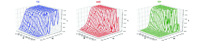
Figure 14: The effect of beacon deployment and node density

We can draw the following conclusions from Fig.14: (1) Node density is the dominant performance factor, especially for TP and WE. (2) A higher beacon density in a network helps finding more localizable nodes. (3) The performance of TP and WE drops sharply when $N$ grows larger than $3.5$ (Fig.14). In contrast, the performance of TE is more stable.

During the above simulations, beacons were placed randomly in the WSNs. We found that the beacon placement could affect the detection when $B\approx 0.01$, as can be seen in the first row of each of the three tables (Tables VII–IX). Fig.15 shows the localizable nodes of a sparse beacon deployment network, a kind of network for which it is difficult to detect the localizable nodes. The network of Fig.15 has only four beacons placed in a $400\times 400$ square ($N=2.0$, $B=0.01$).

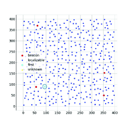
(a) [TE]

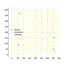
(b) [WE and TP]

Figure 15: Sparse beacon placement

WE and TP could not find any localizable nodes when the beacons were placed much more sparsely, whereas TE still worked well even when only two beacons were closely placed near a flexible node. The first localizable node found by TE was close to the third beacon, as marked in Fig.15.

The simulations demonstrate that the triangle extension (TE) method improves the localizability detection efficiency, especially when sensor nodes are sparsely deployed. Moreover, for each flexible node $v$, TE only requires two non-flexible neighbors for state transitions. In contrast, WE needs at least six edges to set up a wheel graph, and TP needs three edges connected to three localizable neighbors. As a result, not only did TE perform the best among the three algorithms, but it also required the least information about the network.

TABLE III: Hole simulation results

	1	2	3	4	5
TE	0.740	0.855	0.835	0.789	0.797
WE	0.363	0.430	0.499	0.560	0.545
TP	0.148	0.217	0.173	0.247	0.236

We next evaluated the algorithms on networks with holes. A hole of a network is defined as an empty area within the network that has a minimum diameter greater than the transmission range of the nodes. Hence, any two nodes on opposite borders of a hole are not neighbors. Five simulations were performed under the same network deployment with $B=0.1$ and $N=3.2$. To facilitate hole generation, there was no cell partitioning in the networks of these five simulations.

Table III lists the average results of the five simulations. Fig.16 shows the nodes in one of the simulated networks classified by the algorithms. Since the other simulation results are similar, we omit them in the figure. In all simulations, TE detected more localizable nodes than the other two algorithms. To explore the effect of network density $N$ on different algorithms, we further performed simulations on a network with a hole under $N=2.4$ with $B=0.1$. The three algorithms could detect all the localizable nodes in the four corners, but TE was the fastest one to finish when $N=2.4$ and $B=0.1$.

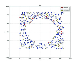
(a) TE

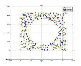
(b) WE

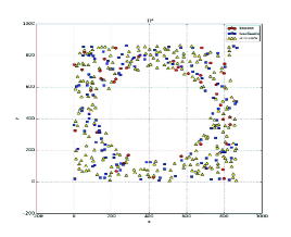
(c) TP

Figure 16: Hole simulation (sparse network) T0: N = 3.2, B =0.1

We then adjusted $B$ to 0.05 and carried out two different beacon deployment distributions, random and skewed, as shown in Fig.17 and Fig.18, respectively. The random beacon deployment is shown in Fig.17. Fig.18 shows that, even with the same beacon density, when beacons were densely deployed in some corners, both TP and WE could work in these corners. In contrast, TE worked in both deployments. It was not affected by the sparse beacon deployment, whether skewed or not.

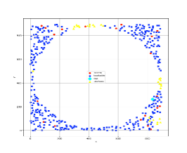
(a) TE

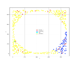
(b) WE

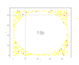
(c) TP

Figure 17: Hole simulation (dense network, random beacon deployment) T1: N = 2.4, B =0.05

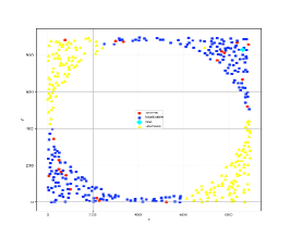
(a) TE

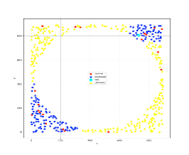
(b) WE

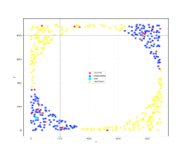
(c) TP

Figure 18: Hole simulation (dense network, skewed beacon deployment) T2: N = 2.4, B =0.05

Finally, we estimated the energy consumption of the algorithms using the execution time and the node electric current. In the energy consumption measurement in VMNet [24], the average electric current of a working node is about 20 mA. The execution time of each algorithm can thus indicate its energy consumption on a sensor node. The simulations were performed under different $N$ and $B$ parameter values. Fig.19 shows the simulation results. The values on the Y-axis are the numbers of run cycles. Suppose the time length of each run cycle is $T$ and an algorithm runs $P$ cycles: The energy consumption of the algorithm is estimated as $E=20~{}(mA)/1000\times 3~{}(V)\times P\times T~{}(s)=0.06PT~{}(J)$, where $3~{}(V)$ is the voltage of the batteries of a sensor node. The algorithms were driven to detect from 25% to 50% of the localizable nodes in a WSN. However, some algorithms failed to reach the required localizability detection percentages. We set a timeout to stop the algorithms as can be seen by the columns that reach the maximum Y (350) in Fig.19. The results show that TE consumed the least energy to find the same number of localizable nodes.

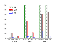
(a) 25% localizable nodes detected

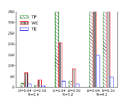
(b) 50% localizable nodes detected

Figure 19: Energy consumption(Unit: 0.06T Joule)

6.2 Experiments

We performed two series of experiments to evaluate the performance of our TE algorithm with up to 14 TelosB wireless sensor nodes. The same detection program was installed on the sensor nodes, each of which was assigned a unique ID. The hardware configuration of a sensor node is listed in Table IV.

TABLE IV: Experiment setup

Operating System:	TinyOS
Processor:	16-bit RISC
Memory:	48 kB Flash and 10KB RAM
Bandwidth:	250 kbps

In order to take photos with all sensor nodes in our experiments, we reduced the node radio power to the minimal level to limit the network deployment area. The photos can thus indicate the status of all the nodes in each network through the LED lights of the sensor nodes. The red, yellow, and blue LED lights are used to represent the three states, flexible, rigid, and localizable, respectively.

6.2.1 Experiment 1

The deployment of the sensor nodes of a WSN in our experiments is shown in Fig.20. The nodes with red light turned on in the figure functioned as beacons. Our manual deployment ensured that certain nodes have to communicate with the beacons via multi-hop. This setup enables nodes to start the direction-extension to construct a triangle block. Otherwise, the nodes in the WSN might either determine their localizability without extension or be theoretically non-localizable.

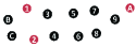
Figure 20: Node deployment in Experiment 1

In the WSNs for the experiments, the three beacons were sequentially set up within three seconds. Then, the pair of beacon nodes 1 and 2 launched the extensions. The LED light switching sequences were recorded manually. The LED light switching sequence corresponds to the temporal order of the state transition events. More specifically, the sequence of switching from red to yellow LED, named as the yellow sequence, indicates the transition from the flexible state to the rigid state; similarly, the blue sequence refers to state transition from the rigid state to the localizable state. The two recorded sequences are listed in Table V. In the table, nodes whose LEDs switched simultaneously are combined as a single element. The yellow sequence took about five seconds, and the blue sequence, three seconds.

TABLE V: Sequences in experiment 1

Yellow sequence	3 and C, 4 and B, 5, 6, 7, 8, 9
Blue sequence	9, 8 and 7, 6 and 5, 3 and 4

The blue sequence finished more quickly as a localizable node also informs a pair of its parents thus spreading the information faster. Fig.21 shows the final status of the whole network. Nodes $B$ and $C$ were not included in the blue sequence because they stayed rigid. The two branches grew in the triangle block, and only one branch could find the third beacon, $A$. The branch containing $B$ and $C$ could not find beacon $A$. In fact, the branch containing $B$ and $C$ is theoretically non-localizable.

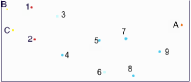
Figure 21: Snapshot of Experiment1

6.2.2 Experiment 2

In this experiment, the sensor nodes were divided into two groups. The IDs and approximate locations of the sensor nodes are shown in Fig.22. The distance between groups was changed to test the Dual-V-Topo scenario and to verify that our dual-v-detection method works. In each group, two nodes were chosen as a pair of beacons to launch extensions. To reproduce the meeting of two triangle blocks, two nodes in different groups could not receive messages from each other initially. After each group finished constructing its own triangle block, some border nodes in one group would be moved closer to the other group. Consequently, the two groups could form a Dual-V-Topo.

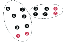
Figure 22: Node deployment in Experiment2

In the WSN of Fig.22, we moved the rigid nodes D and E closer to rigid nodes 5 and 7. Table VI lists the blue sequences of the two groups. It can be seen from the table that dual-v-detection is able to detect the localizability of nodes in the meeting area. Each node in the meeting area collected the messages from two nodes in the different triangle blocks and then sent a query message to its neighbors. In this experiment, node E communicated with nodes 7 and 5. Node E inquired of its parent D whether node D could also communicate with node 7 or 5. Node E informed node D of the success of the dual-v-detection process when node D replied with a confirmation message to node E. Then, the rigid nodes in this group sequentially turned on blue LED lights, indicating that these rigid nodes were all localizable.

TABLE VI: Blue sequences in Experiment 2

Left group	7 and 5, 6 and 4, 3
Right group	E and D, C and B

Fig.23 shows the final LED light status of the WSN in Experiment 2. In this figure, the LED light of node 8 is yellow although that of its parent, node 7, is blue. The reason is that the localizability of a node does not help its child to detect its localizability but instead helps its ancestors to detect their localizability. Consequently, as node 7 is the parent of node 8, node 8 could not be determined as localizable even though node 7 is localizable.

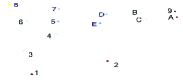
Figure 23: Snapshot of Experiment2

7 Conclusion and Future Work

Determining theoretically localizable and non-localizable nodes in a WSN is important for most localization algorithms and applications. In this paper, we propose a distributed algorithm, TE, to determine the localizable nodes in a network based on graph rigidity theory. TE uses an efficient approach of triangle extension to construct a rigid graph to detect the localizable nodes and needs less information than the existing algorithms. We theoretically analyzed the efficiency of TE and compared it to that of the existing algorithms. Simulations and experiments also demonstrated that TE is applicable to real-world WSNs. A promising direction is to integrate TE with localization algorithms.

Appendix A Proof of Lemma 1

Proof.

During an extension operation process, suppose a node, denoted as $v$, $v\notin V_{G}$, is added to $V_{G}$ and edges $(v,v_{1}),(v,v_{2}),(v_{1},v_{2})\in V_{G}$ are added to $E_{G}$. Now a new graph $G_{1}$ is created after the extension. As $G$ is minimally rigid, it has $|E_{G}|=2|V_{G}|-3$; since $|V_{G_{1}}|=|V_{G}|+1$ and $|E_{G_{1}}|=|E_{G}|+2$, Equation (1) can be derived:

$|E_{G_{1}}|=2|V_{G_{1}}|-3~{}~{}~{}~{}~{}~{}~{}~{}~{}~{}~{}~{}~{}~{}~{}~{}~{}~{}~{}~{}~{}~{}~{}~{}~{}~{}~{}~{}~{}~{}~{}~{}~{}~{}~{}~{}~{}$(1)

With equation (1), we now only need to prove the following condition according to Laman’s Lemma to prove $G_{1}$ is minimally rigid: $|E[X]|\leq 2|X|-3$ for each $X\subset V_{G_{1}}$ with $2\leq|X|\leq|V_{G_{1}}|-1$.

If $v\notin X$, $X\subset V_{G}$, then according to Laman’s Lemma, $|E[X]|\leq 2|X|-3$, since $G$ is minimally rigid.

If $v\in X$, we prove by contradiction. Suppose $|E[X]|>2|X|-3$. We first remove node $i$ from $X$ and up to two relevant edges from $E[X]$. Then, $|E[X]|>2|X|-3$ is still true. However, this contradicts the given condition that $G$ is minimally rigid and thus $|E[X]|\leq 2|X|-3$, since $X\in V_{G}$ after the removal. Therefore, $G_{1}$ is minimally rigid. ∎

Appendix B Numeric results in simulations

This section gives the numeric values in our simulation, as mentioned in Section6.1.

TABLE VII: Proportion of localizable nodes found by TE

	2.0	2.2	2.4	2.6	2.8	3.0	3.2	3.4	3.6	3.8	4.0	4.2	4.4	4.6	4.8	5.0	5.2	5.4	5.6	5.8
0.01	0.666	0.332	0.994	0.665	0.332	0.329	0.549	0.636	0.000	0.000	0.168	0.000	0.000	0.000	0.000	0.000	0.000	0.000	0.000	0.000
0.02	0.999	0.996	0.997	0.956	0.999	0.931	0.969	0.991	0.644	0.300	0.429	0.395	0.171	0.000	0.000	0.000	0.000	0.000	0.000	0.000
0.03	0.991	0.996	0.993	0.973	0.997	0.978	0.957	0.973	0.897	0.954	0.627	0.552	0.193	0.033	0.000	0.000	0.007	0.014	0.000	0.000
0.04	0.999	0.949	0.997	0.996	0.953	0.993	0.973	0.976	0.957	0.818	0.910	0.543	0.296	0.166	0.025	0.016	0.008	0.000	0.000	0.000
0.05	0.992	0.989	0.995	0.984	0.988	0.996	0.992	0.980	0.968	0.958	0.822	0.715	0.423	0.154	0.037	0.054	0.047	0.000	0.000	0.001
0.06	0.992	0.994	0.996	0.999	0.976	0.989	0.991	0.996	0.973	0.954	0.941	0.821	0.537	0.137	0.095	0.082	0.016	0.020	0.002	0.000
0.07	0.988	0.992	0.994	0.990	0.996	0.969	0.993	0.987	0.963	0.945	0.884	0.800	0.686	0.415	0.165	0.116	0.018	0.000	0.000	0.014
0.08	0.998	0.998	0.989	0.989	0.992	0.973	0.986	0.979	0.988	0.964	0.940	0.880	0.717	0.375	0.254	0.037	0.043	0.039	0.004	0.005
0.09	1.000	0.994	0.997	0.988	0.993	0.989	0.986	0.978	0.989	0.984	0.908	0.853	0.750	0.483	0.210	0.117	0.046	0.070	0.016	0.005
0.1	0.988	0.994	0.990	0.996	0.994	0.996	0.992	0.996	0.970	0.972	0.944	0.854	0.722	0.523	0.318	0.125	0.074	0.028	0.020	0.004
0.11	0.987	0.992	0.993	0.993	0.998	0.975	0.996	0.985	0.988	0.978	0.917	0.874	0.707	0.538	0.266	0.141	0.075	0.052	0.043	0.024
0.12	0.995	0.997	0.995	0.998	0.993	0.994	0.988	0.986	0.980	0.973	0.964	0.906	0.826	0.630	0.371	0.296	0.132	0.044	0.031	0.006
0.13	0.995	0.995	0.997	0.997	0.995	0.988	0.989	0.969	0.988	0.969	0.972	0.856	0.732	0.712	0.314	0.223	0.106	0.123	0.037	0.023
0.14	0.999	0.996	0.996	0.999	0.987	0.997	0.995	0.996	0.990	0.997	0.962	0.912	0.830	0.621	0.459	0.303	0.102	0.058	0.038	0.033
0.15	0.992	0.994	0.995	0.998	0.998	0.990	0.993	0.997	0.988	0.978	0.950	0.919	0.855	0.742	0.383	0.289	0.165	0.090	0.052	0.052
0.16	0.994	0.998	1.000	0.996	0.999	0.985	0.998	0.985	0.979	0.974	0.968	0.922	0.819	0.699	0.434	0.311	0.247	0.150	0.045	0.051
0.17	0.994	1.000	0.996	0.995	0.995	0.998	0.995	0.989	0.981	0.990	0.971	0.925	0.856	0.690	0.453	0.339	0.247	0.119	0.047	0.034
0.18	0.998	0.998	0.997	0.997	0.990	0.998	0.981	0.996	0.990	0.977	0.958	0.918	0.831	0.768	0.557	0.409	0.169	0.189	0.078	0.042
0.19	0.999	0.999	1.000	1.000	0.999	0.999	0.996	0.995	0.989	0.965	0.962	0.954	0.853	0.711	0.565	0.403	0.259	0.154	0.069	0.100
0.2	0.998	0.995	0.998	0.999	0.999	0.996	0.997	0.995	0.993	0.980	0.976	0.940	0.876	0.748	0.599	0.424	0.256	0.147	0.118	0.059

TABLE VIII: Proportion of localizable nodes found by TP

	2.0	2.2	2.4	2.6	2.8	3.0	3.2	3.4	3.6	3.8	4.0	4.2	4.4	4.6	4.8	5.0	5.2	5.4	5.6	5.8
0.01	0.000	0.000	0.000	0.000	0.000	0.000	0.000	0.000	0.000	0.000	0.000	0.000	0.000	0.000	0.000	0.000	0.000	0.000	0.000	0.000
0.02	0.333	0.333	0.000	0.000	0.000	0.000	0.000	0.000	0.000	0.000	0.000	0.000	0.000	0.000	0.000	0.000	0.000	0.000	0.000	0.000
0.03	0.000	0.333	0.332	0.333	0.000	0.000	0.329	0.000	0.000	0.000	0.000	0.000	0.000	0.000	0.000	0.000	0.000	0.000	0.000	0.000
0.04	1.000	1.000	0.333	0.000	0.000	0.000	0.272	0.194	0.000	0.000	0.000	0.000	0.000	0.000	0.000	0.000	0.000	0.000	0.000	0.000
0.05	1.000	1.000	1.000	1.000	1.000	0.332	0.650	0.061	0.000	0.001	0.000	0.000	0.000	0.000	0.000	0.000	0.000	0.000	0.000	0.000
0.06	1.000	1.000	1.000	0.667	0.998	0.998	0.326	0.515	0.161	0.000	0.000	0.004	0.000	0.000	0.000	0.000	0.000	0.000	0.000	0.000
0.07	1.000	1.000	1.000	0.999	1.000	0.329	0.658	0.731	0.050	0.030	0.012	0.002	0.005	0.000	0.000	0.000	0.000	0.000	0.000	0.000
0.08	1.000	1.000	0.999	1.000	0.999	0.998	0.989	0.289	0.189	0.021	0.000	0.000	0.000	0.000	0.000	0.000	0.003	0.000	0.000	0.000
0.09	1.000	1.000	1.000	1.000	1.000	0.998	0.990	0.781	0.279	0.000	0.025	0.002	0.013	0.000	0.000	0.000	0.000	0.000	0.000	0.000
0.1	1.000	1.000	1.000	1.000	0.999	0.995	0.986	0.866	0.495	0.130	0.042	0.014	0.002	0.003	0.001	0.001	0.000	0.000	0.000	0.000
0.11	1.000	1.000	1.000	1.000	1.000	0.999	0.991	0.978	0.568	0.111	0.021	0.016	0.011	0.004	0.002	0.000	0.000	0.000	0.000	0.000
0.12	1.000	1.000	1.000	1.000	1.000	0.996	0.989	0.906	0.697	0.137	0.053	0.020	0.004	0.001	0.001	0.001	0.000	0.004	0.001	0.000
0.13	1.000	1.000	1.000	0.998	0.999	0.997	0.994	0.953	0.678	0.261	0.102	0.043	0.010	0.005	0.004	0.003	0.003	0.000	0.001	0.000
0.14	1.000	1.000	1.000	1.000	0.999	0.997	0.996	0.979	0.801	0.329	0.130	0.047	0.008	0.007	0.003	0.000	0.002	0.002	0.000	0.000
0.15	1.000	1.000	1.000	1.000	0.999	0.996	0.987	0.963	0.825	0.370	0.125	0.070	0.040	0.023	0.004	0.002	0.002	0.002	0.002	0.003
0.16	1.000	1.000	1.000	1.000	0.999	0.999	0.993	0.954	0.827	0.365	0.162	0.123	0.029	0.025	0.010	0.002	0.001	0.003	0.001	0.000
0.17	1.000	1.000	1.000	1.000	0.998	0.999	0.989	0.945	0.769	0.367	0.252	0.101	0.049	0.017	0.016	0.013	0.006	0.003	0.003	0.000
0.18	1.000	1.000	1.000	0.999	1.000	0.994	0.989	0.968	0.771	0.646	0.292	0.081	0.030	0.019	0.014	0.001	0.001	0.004	0.002	0.002
0.19	1.000	1.000	0.999	1.000	0.999	1.000	0.985	0.969	0.903	0.714	0.271	0.119	0.044	0.029	0.017	0.004	0.007	0.001	0.004	0.001
0.2	1.000	1.000	1.000	1.000	0.999	0.997	0.986	0.978	0.893	0.655	0.308	0.108	0.062	0.028	0.009	0.009	0.006	0.002	0.002	0.005

TABLE IX: Proportion of localizable nodes found by WE

	2.0	2.2	2.4	2.6	2.8	3.0	3.2	3.4	3.6	3.8	4.0	4.2	4.4	4.6	4.8	5.0	5.2	5.4	5.6	5.8
0.01	0.000	0.000	0.000	0.000	0.000	0.000	0.000	0.000	0.000	0.000	0.000	0.000	0.000	0.000	0.000	0.000	0.000	0.000	0.000	0.000
0.02	0.667	0.333	0.000	0.000	0.000	0.000	0.097	0.000	0.000	0.000	0.000	0.008	0.000	0.000	0.000	0.000	0.000	0.000	0.000	0.000
0.03	0.336	0.667	0.155	0.333	0.199	0.000	0.033	0.025	0.000	0.000	0.000	0.000	0.000	0.000	0.000	0.000	0.000	0.000	0.000	0.000
0.04	1.000	1.000	0.661	0.353	0.077	0.284	0.070	0.048	0.027	0.000	0.000	0.000	0.000	0.000	0.005	0.000	0.000	0.000	0.000	0.000
0.05	1.000	1.000	0.931	0.997	0.877	0.527	0.220	0.138	0.000	0.000	0.016	0.023	0.000	0.000	0.000	0.000	0.012	0.002	0.000	0.000
0.06	1.000	1.000	1.000	0.995	0.952	0.443	0.390	0.086	0.069	0.064	0.031	0.023	0.000	0.009	0.004	0.000	0.008	0.003	0.003	0.000
0.07	1.000	1.000	1.000	1.000	0.997	0.646	0.377	0.294	0.177	0.081	0.062	0.074	0.011	0.014	0.014	0.025	0.000	0.000	0.004	0.004
0.08	1.000	1.000	1.000	1.000	0.990	0.987	0.571	0.239	0.267	0.139	0.038	0.050	0.025	0.044	0.014	0.002	0.013	0.000	0.000	0.000
0.09	1.000	1.000	1.000	1.000	0.986	0.931	0.435	0.416	0.285	0.100	0.122	0.043	0.055	0.028	0.026	0.002	0.019	0.009	0.004	0.005
0.1	1.000	1.000	1.000	0.999	0.999	0.959	0.744	0.637	0.247	0.319	0.169	0.055	0.095	0.073	0.014	0.024	0.009	0.005	0.010	0.004
0.11	1.000	1.000	1.000	1.000	0.999	0.981	0.884	0.630	0.400	0.170	0.145	0.085	0.083	0.072	0.018	0.021	0.003	0.010	0.008	0.004
0.12	1.000	1.000	1.000	1.000	0.996	0.975	0.826	0.680	0.420	0.285	0.262	0.113	0.131	0.048	0.051	0.022	0.013	0.015	0.018	0.015
0.13	1.000	1.000	1.000	1.000	1.000	0.989	0.842	0.716	0.637	0.488	0.258	0.187	0.119	0.055	0.039	0.032	0.035	0.007	0.017	0.007
0.14	1.000	1.000	0.999	1.000	0.999	0.963	0.939	0.818	0.676	0.513	0.321	0.221	0.141	0.089	0.081	0.045	0.037	0.032	0.004	0.018
0.15	1.000	1.000	1.000	1.000	1.000	0.995	0.946	0.844	0.757	0.537	0.396	0.291	0.169	0.121	0.109	0.111	0.023	0.046	0.017	0.013
0.16	1.000	1.000	0.999	1.000	1.000	0.998	0.947	0.785	0.694	0.541	0.453	0.266	0.145	0.133	0.100	0.054	0.057	0.058	0.024	0.022
0.17	1.000	1.000	1.000	0.999	0.999	0.989	0.954	0.854	0.738	0.658	0.442	0.418	0.222	0.117	0.090	0.104	0.062	0.040	0.039	0.015
0.18	1.000	1.000	1.000	1.000	1.000	0.984	0.994	0.892	0.777	0.616	0.474	0.348	0.222	0.150	0.146	0.083	0.032	0.073	0.033	0.032
0.19	1.000	1.000	1.000	0.999	0.999	0.999	0.984	0.987	0.870	0.746	0.540	0.381	0.281	0.182	0.172	0.098	0.114	0.057	0.043	0.048
0.2	1.000	1.000	1.000	1.000	1.000	0.998	0.994	0.952	0.710	0.795	0.527	0.426	0.311	0.279	0.166	0.152	0.083	0.065	0.053	0.041

Hejun Wu received his Ph.D. degree in Computer Science and Engineering from Hong Kong University of Science and Technology in 2008. He is currently an Associate Professor with the School of Data and Computer Science, Sun Yat-sen University, Guangzhou, China. His main research interests include Wireless Sensor Networks and Distributed Computing. He is a member of the IEEE and ACM.

Ao Ding received the B.S degree in computer science from Anhui University in 2014 and the M.Phil degree in computer science from Sun Yat-Sen University in 2017. His research interests include wireless sensor networks, distributed computing, and machine learning.

Weiwei Liu received the B.S degree in computer science from Southeast University in 2011 and the M.Phil degree from Sun Yat-Sen University in 2014. He is currently with Horizon Robotics as a system engineer and major in automatic driving system development, including system design, HD map generating and vehicle trajectory planning. His research interests includes nature language processing, trajectory planning and ad-hoc network localization.

Lvzhou Li Lvzhou Li received the Ph.D. degree in computer science from Sun Yat-Sen University, Guangzhou, China, in 2009. He is currently an Associate Professor with the School of Data and Computer Science, Sun Yat-sen University, Guangzhou, China. His current research interests include theoretical computer science and quantum computing.

Zheng Yang (M’11) received the B.E. degree in computer science from Tsinghua University in 2006 and the Ph.D. degree in computer science from Hong Kong University of Science and Technology in 2010. He is currently an associate professor with Tsinghua University. His main research interests include wireless ad-hoc/sensor networks and mobile computing. He is a member of the IEEE and ACM.

References

- [1] K. K. Almuzaini and T. A. Gulliver. Range-based localization in wireless networks using the dbscan clustering algorithm. In VTC Spring, pages 1–7. IEEE, 2011.
- [2] A. R. Berg and T. Jord¨¢n. Algorithms for graph rigidity and scene analysis. In G. D. Battista and U. Zwick, editors, ESA, volume 2832 of Lecture Notes in Computer Science, pages 78–89. Springer, 2003.
- [3] A. R. Berg and T. Jord¨¢n. A proof of connelly’s conjecture on 3-connected circuits of the rigidity matroid. J. Comb. Theory, Ser. B, 88(1):77–97, 2003.
- [4] Y. Chen, D. Lymberopoulos, J. Liu, and B. Priyantha. Indoor localization using fm signals. IEEE Trans. Mob. Comput., 12(8):1502–1517, 2013.
- [5] T. Eren, D. K. Goldenberg, W. Whiteley, Y. R. Yang, A. S. Morse, B. D. O. Anderson, and P. N. Belhumeur. Rigidity, computation, and randomization in network localization. In INFOCOM, 2004.
- [6] T. Eren, Graph invariants for unique localizability in cooperative localization of wireless sensor networks: rigidity index and redundancy index. Ad Hoc Networks, 44: 32-45, 2016.
- [7] S. Han and Z. Gong and W. Meng and C. Li and D. Zhang and W. Tang. Automatic Precision Control Positioning for Wireless Sensor Network. In Sensors Journal, 16(7): pages 2140–2150. IEEE, 2016.
- [8] Longfei Shangguan, Zheng Yang, Alex X. Liu, Zimu Zhou, Yunhao Liu, STPP: Spatial-Temporal Phase Profiling-Based Method for Relative RFID Tag Localization, IEEE/ACM Transactions on Networking (ToN), 25(1): pages 596-609, 2017.
- [9] Zheng Yang, Chenshu Wu, Zimu Zhou, Xinglin Zhang, Xu Wang, Yunhao Liu, Mobility Increases Localizability: A Survey on Wireless Indoor Localization using Inertial Sensors, ACM Computing Surveys, 47(3), Article No. 54, 2015.
- [10] B. Hendrickson. Conditions for unique graph realizations. SIAM J. Comput., 21(1):65–84, 1992.
- [11] B. Jackson and T. Jordán. Connected rigidity matroids and unique realizations of graphs. J. Comb. Theory, Ser. B, 94(1):1–29, 2005.
- [12] B. Jackson and T. Jord¨¢n. Connected rigidity matroids and unique realizations of graphs. J. Comb. Theory, Ser. B, 94(1):1–29, 2005.
- [13] G. Laman. On graphs and rigidity of plane skeletal structures. J. Engrg. Math., 4:331–340, 1970.
- [14] P. Levis, N. LEE, M. Welsh, and D. Culler. TOSSIM: Accurate and scalable simulation of entire TinyOS applications. Proceedings of the 1st international conference on Embedded networked sensor systems., pages 126–137. ACM, 2003.
- [15] P. Levis, S. Madden, J. Polastre, R. Szewczyk, K. Whitehouse, A. Woo, D. Gay, J. Hills, M. Welsh, E. Brewer, and D. Culler. Tinyos: An operating system for sensor networks. Ambient intelligence., pages 115–148. Springer Berlin Heidelberg, 2005.
- [16] L. Lazos and R. Poovendran. Hirloc: high-resolution robust localization for wireless sensor networks. IEEE Journal on Selected Areas in Communications, 24(2):233–246, 2006.
- [17] Z. Ma, W. Chen, K. B. Letaief, and Z. Cao. A semi range-based iterative localization algorithm for cognitive radio networks. IEEE Transactions on Vehicular Technology., pages 704–717, 2010.
- [18] D. C. Moore, J. J. Leonard, D. Rus, and S. J. Teller. Robust distributed network localization with noisy range measurements. In J. A. Stankovic, A. Arora, and R. Govindan, editors, SenSys, pages 50–61. ACM, 2004.
- [19] D. Niculescu and B. Nath. Dv based positioning in ad hoc networks. Telecommunication Systems, 22(1-4):267–280, 2003.
- [20] N. B. Priyantha, A. Chakraborty, and H. Balakrishnan. The cricket location-support system. In MOBICOM, pages 32–43, 2000.
- [21] A. Savvides, C.-C. Han, and M. Srivastava. Dynamic fine-grained localization in ad-hoc networks of sensors. In Proceedings of the ACM International Conference on Mobile Computing and Networking, pages 166–179, Rome, Italy, July 2001. ACM.
- [22] J. Schloemann , H. S. Dhillon, R. M. Buehrer. A tractable analysis of the improvement in unique localizability through collaboration. IEEE Transactions on Wireless Communications,15(6): 3934-3948, 2016.
- [23] S. Seidel and T. Rappaport. 914 mhz path loss prediction models for indoor wireless communications in multifloored buildings. Antennas and Propagation, IEEE Transactions on, 40(2):207–217, 1992.
- [24] H. Wu, Q. Luo, P. Zheng and L. M. Ni. VMNet: Realistic Emulation of Wireless Sensor Networks. In IEEE Trans. Parallel Distrib. Syst. , 18(2): 277-288, 2007.
- [25] N. Xia, Y. Ou, S. Wang, R. Zheng, H. Du. Localizability Judgment in UWSNs Based on Skeleton and Rigidity Theory. IEEE Transactions on Mobile Computing, 2016.
- [26] Z. Yang and Y. Liu. Understanding node localizability of wireless ad hoc and sensor networks. IEEE Trans. Mob. Comput., 11(8):1249–1260, 2012.
- [27] Z. Yang, Y. Liu, and X.-Y. Li. Beyond trilateration: On the localizability of wireless ad-hoc networks. In INFOCOM, pages 2392–2400. IEEE, 2009.