A Spectral Element Reduced Basis Method for Navier-Stokes Equations with Geometric Variations

Abstract

We consider the Navier-Stokes equations in a channel with a narrowing of varying height. The model is discretized with high-order spectral element ansatz functions, resulting in $6372$ degrees of freedom. The steady-state snapshot solutions define a reduced order space through a standard POD procedure. The reduced order space allows to accurately and efficiently evaluate the steady-state solutions for different geometries. In particular, we detail different aspects of implementing the reduced order model in combination with a spectral element discretization. It is shown that an expansion in element-wise local degrees of freedom can be combined with a reduced order modelling approach to enhance computational times in parametric many-query scenarios.

1 Introduction and Motivation

Spectral element methods (SEM) use high-order polynomial ansatz functions to solve partial differential equations (PDEs) in all fields of science and engineering, see, e.g., Hess:Sherwin:2005 ; Hess:CHQZ1 ; Hess:CHQZ2 ; Hess:PateraSEM ; Hess:Herrero2013132 ; Hess:Taddei and references therein for an overview. Typically, an exponential error decay under p-refinement is observed, which can provide an enhanced accuracy over standard finite element methods at the same computational cost. In the following, we assume that the discretization error is much smaller than the model reduction error, small enough not to interfere with our results. In general, this needs to be established with the use of suitable error estimation and adaptivity techniques.

We consider the flow through a channel with a narrowing of variable height. A reduced order model (ROM) is computed from a few high-order SEM solves, which accurately approximates the high-order solutions for the parameter range of interest, i.e., the different narrowing heights under consideration. Since the parametric variations are affine, a mapping to a reference domain is applied without further interpolation techniques. The focus of this work is to show how to use simulations arising from the SEM solver Nektar++ Hess:nektar in a ROM context. In particular, the multilevel static condensation of the high-order solver is not applied, but the ROM projection works with the system matrices in local coordinates. See Hess:Sherwin:2005 for further details. This is in contrast to our previous work Hess:ENUMATH17_me , since numerical experiments have shown that the multilevel static condensation is inefficient in a ROM context. Additionally, we consider affine geometry variations. With SEM as discretization method, we use global approximation functions for the high-order as well as reduced-order methods. The ROM techniques described in this paper are implemented in open-source project ITHACA-SEM.

The outline of the paper is as follows. In Sec. 2, the model problem is defined and the geometric variations are introduced. Sec. 3 provides details on the spectral element discretization, while Sec. 4 describes the model reduction approach and shows the affine mapping to the reference domain. Numerical results are given in Sec. 5, while Sec. 6 summarizes the work and points out future perspectives.

2 Problem Formulation

Let $\Omega\in\mathbb{R}^{2}$ be the computational domain. Incompressible, viscous fluid motion in spatial domain $\Omega$ over a time interval $(0,T)$ is governed by the incompressible Navier-Stokes equations with vector-valued velocity $\mathbf{u}$, scalar-valued pressure $p$, kinematic viscosity $\nu$ and a body forcing $\mathbf{f}$:

$$\frac{\partial\mathbf{u}}{\partial t}+\mathbf{u}\cdot\nabla\mathbf{u} = -\nabla p+\nu\Delta\mathbf{u}+\mathbf{f},$$ (1)

$$\nabla\cdot\mathbf{u} = 0.$$ (2)

Boundary and initial conditions are prescribed as

$$\mathbf{u} = \mathbf{d}\quad\text{ on }\Gamma_{D}\times(0,T),$$ (3)

$$\nabla\mathbf{u}\cdot\mathbf{n} = \mathbf{g}\quad\text{ on }\Gamma_{N}\times(0,T),$$ (4)

$$\mathbf{u} = \mathbf{u}_{0}\quad\text{ in }\Omega\times 0,$$ (5)

with $\mathbf{d}$, $\mathbf{g}$ and $\mathbf{u}_{0}$ given and $\partial\Omega=\Gamma_{D}\cup\Gamma_{N}$, $\Gamma_{D}\cap\Gamma_{N}=\emptyset$. The Reynolds number $Re$, which characterizes the flow Hess:Holmes , depends on $\nu$, a characteristic velocity $U$, and a characteristic length $L$:

$$Re=\frac{UL}{\nu}.$$ (6)

We are interested in computing the steady states, i.e., solutions where $\frac{\partial\mathbf{u}}{\partial t}$ vanishes. The high-order simulations are obtained through time-advancement, while the ROM solutions are obtained with a fixed-point iteration.

2.1 Oseen-Iteration

The Oseen-iteration is a secant modulus fixed-point iteration, which in general exhibits a linear rate of convergence Hess:Oseen . Given a current iterate (or initial condition) $\mathbf{u}^{k}$, the next iterate $\mathbf{u}^{k+1}$ is found by solving linear system:

$$-\nu\Delta\mathbf{u}^{k+1}+(\mathbf{u}^{k}\cdot\nabla)\mathbf{u}^{k+1}+\nabla p = \mathbf{f}\text{ in }\Omega,$$

$$\nabla\cdot\mathbf{u}^{k+1} = 0\text{ in }\Omega,$$

$$\mathbf{u}^{k+1} = \mathbf{d}\quad\text{ on }\Gamma_{D},$$

$$\nabla\mathbf{u}^{k+1}\cdot\mathbf{n} = \mathbf{g}\quad\text{ on }\Gamma_{N}.$$

Iterations are typical stopped when the relative difference between iterates falls below a predefined tolerance in a suitable norm, like the $L^{2}(\Omega)$ or $H^{1}_{0}(\Omega)$ norm.

2.2 Model Description

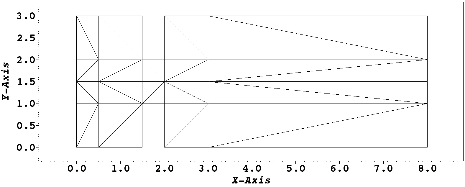
Figure 1: Reference computational domain for the channel flow, divided into $36$ triangles.

We consider the reference computational domain shown in Fig. 1, which is decomposed into $36$ triangular spectral elements. The spectral element expansion uses modal Legendre polynomials of the Koornwinder-Dubiner type of order $p=11$ for the velocity. Details on the discretization method can be found in chapter 3.2 of Hess:Sherwin:2005 . The pressure ansatz space is chosen of order $p-2$ to fulfill the inf-sup stability condition Hess:BBF ; Hess:infsup . A parabolic inflow profile is prescribed at the inlet (i.e., $x=0$) with horizontal velocity component $u_{x}(0,y)=y(3-y)$ for $y\in[0,3]$. At the outlet (i.e $x=8$) we impose a stress-free boundary condition, everywhere else we prescribe a no-slip condition.

The height of the narrowing in the reference configuration is $\mu=1$, from $y=1$ to $y=2$. See Fig. 1. Parameter $\mu$ is considered variable in the interval $\mu\in[0.1,2.9]$. The narrowing is shrunken or expanded as to maintain the geometry symmetric about line $y=1.5$. Fig. 2, Fig. 3, and Fig. 4 show the velocity components close to the the steady state for $\mu=1,0.1,2.9$, respectively.

   

   

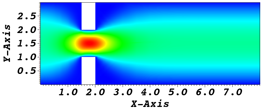
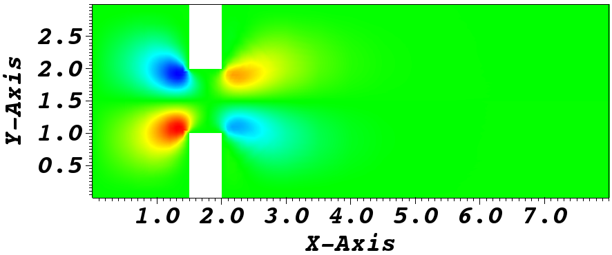
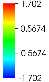
Figure 2: Full order, steady-state solution for $\mu=1$: velocity in x-direction (top) and y-direction (bottom).

   

   

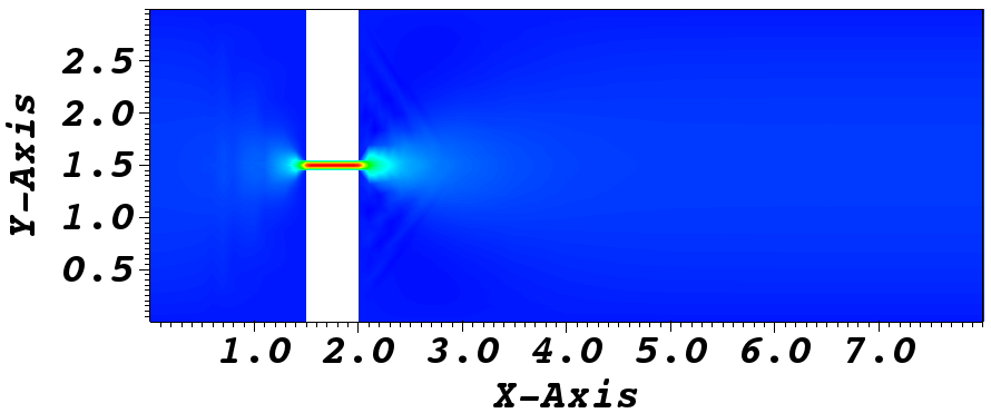
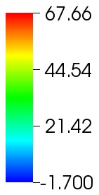
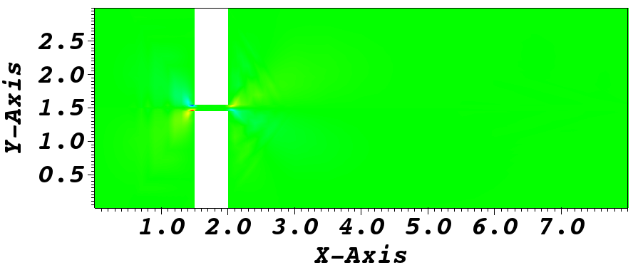
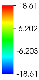
Figure 3: Full order, steady-state solution for $\mu=0.1$: velocity in x-direction (top) and y-direction (bottom).

   

   

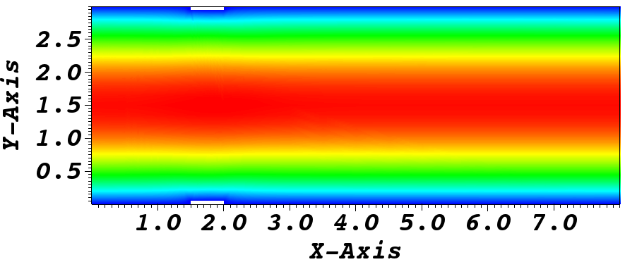
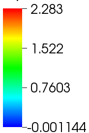
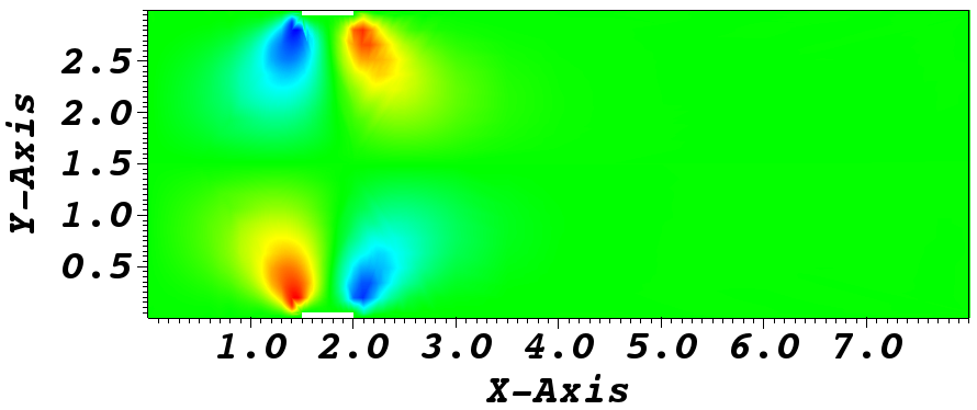
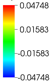
Figure 4: Full order, steady-state solution for $\mu=2.9$: velocity in x-direction (top) and y-direction (bottom).

The viscosity is kept constant to $\nu=1$. For these simulations, the Reynolds number (6) is between $5$ and $10$, with maximum velocity in the narrowing as characteristic velocity $U$ and the height of the narrowing characteristic length $L$. For larger Reynolds numbers (about $30$), a supercritical pitchfork bifurcation occurs giving rise to the so-called Coanda effect Hess:wille_fernholz_1965 ; Hess:max_bif ; Hess:ENUMATH17_me , which is not subject of the current study. Our model is similar to the model considered in Hess:Pitton2017534 , i.e. an expansion channel with an inflow profile of varying height. However, in Hess:Pitton2017534 the computational domain itself does not change.

3 Spectral Element Full Order Discretization

The Navier-Stokes problem is discretized with the spectral element method. The spectral/hp element software framework used is Nektar++ in version 4.4.0. The discretized system of size $N_{\delta}$ to solve at each step of the Oseen-iteration for fixed $\mu$ can be written as

$$\begin{bmatrix}\begin{array}[]{ccc}A&-D^{T}_{bnd}&B\\ -D_{bnd}&0&-D_{int}\\ \tilde{B}^{T}&-D^{T}_{int}&C\end{array}\end{bmatrix}\begin{bmatrix}\begin{array}[]{ccc}\mathbf{v}_{bnd}\\ \mathbf{p}\\ \mathbf{v}_{int}\end{array}\end{bmatrix} =\begin{bmatrix}\begin{array}[]{ccc}\mathbf{f}_{bnd}\\ \mathbf{0}\\ \mathbf{f}_{int}\end{array}\end{bmatrix},$$ (7)

where $\mathbf{v}_{bnd}$ and $\mathbf{v}_{int}$ denote velocity degrees of freedom on the boundary and in the interior of the domain, respectively, while $\mathbf{p}$ denotes the pressure degrees of freedom. The forcing terms on the boundary and interior are denoted by $\mathbf{f}_{bnd}$ and $\mathbf{f}_{int}$, respectively. The matrix $A$ assembles the boundary-boundary coupling, $B$ the boundary-interior coupling, $\tilde{B}$ the interior-boundary coupling, and $C$ assembles the interior-interior coupling of elemental velocity ansatz functions. In the case of a Stokes system, it holds that $B=\tilde{B}^{T}$, but this is not the case for the Oseen equation because of the linearized convective term. The matrices $D_{bnd}$ and $D_{int}$ assemble the pressure-velocity boundary and pressure-velocity interior contributions, respectively.

The linear system (7) is assembled in local degrees of freedom, resulting in block matrices $A,B,\tilde{B},C,D_{bnd}$ and $D_{int}$, each block corresponding to a spectral element. This allows for an efficient matrix assembly since each spectral element is independent from the others, but makes the system singular. In order to solve the system, the local degrees of freedom need to be gathered into the global degrees of freedom Hess:Sherwin:2005 .

The high-order element solver Nektar++ uses a multilevel static condensation for the solution of linear systems like (7). Since static condensation introduces intermediate parameter-dependent matrix inversions (such as $C^{-1}$ in this case) several intermediate projection spaces need to be introduced to use model order reduction Hess:ENUMATH17_me . This can be avoided by instead projecting the expanded system (7) directly. The internal degrees of freedom do not need to be gathered, since they are the same in local and global coordinates. Only ansatz functions extending over multiple spectral elements need to be gathered.

Next, we will take the boundary-boundary coupling across element interfaces into account. Let $M$ denote the rectangular matrix which gathers the local boundary degrees of freedom into global boundary degrees of freedom. Multiplication of the first row of (7) by $M^{T}M$ will then set the boundary-boundary coupling in local degrees of freedom:

$$\begin{bmatrix}\begin{array}[]{ccc}M^{T}MA&-M^{T}MD^{T}_{bnd}&M^{T}MB\\ -D_{bnd}&0&-D_{int}\\ \tilde{B}^{T}&-D^{T}_{int}&C\end{array}\end{bmatrix}\begin{bmatrix}\begin{array}[]{ccc}\mathbf{v}_{bnd}\\ \mathbf{p}\\ \mathbf{v}_{int}\end{array}\end{bmatrix} =\begin{bmatrix}\begin{array}[]{ccc}M^{T}M\mathbf{f}_{bnd}\\ \mathbf{0}\\ \mathbf{f}_{int}\end{array}\end{bmatrix}.$$ (8)

The action of the matrix in (8) on the degrees of freedom on the Dirichlet boundary is computed and added to the right hand side. Such degrees of freedom are then removed from (8). The resulting system can then be used in a projection-based ROM context Hess:Lassila2014 , of high-order dimension $N_{\delta}\times N_{\delta}$ and depending on the parameter $\mu$ :

$$\mathcal{A}(\mu)\mathbf{x}(\mu)=\mathbf{f}.$$ (9)

4 Reduced Order Model

The reduced order model (ROM) computes accurate approximations to the high-order solutions in the parameter range of interest, while greatly reducing the overall computational time. This is achieved by two ingredients. First, a few high-order solutions are computed and the most significant proper orthogonal decomposition (POD) modes are obtained Hess:Lassila2014 . These POD modes define the reduced order ansatz space of dimension $N$, in which the system is solved. Second, to reduce the computational time, an offline-online computational procedure is used. See Sec. 4.1.

The POD computes a singular value decomposition of the snapshot solutions to $99.99\%$ of the most dominant modes Hess:RBref , which define the projection matrix $U\in\mathbb{R}^{N_{\delta}\times N}$ used to project system (9):

$$U^{T}\mathcal{A}(\mu)U\mathbf{x}_{N}(\mu)=U^{T}\mathbf{f}.$$ (10)

The low order solution $\mathbf{x}_{N}(\mu)$ then approximates the high order solution as $\mathbf{x}(\mu)\approx U\mathbf{x}_{N}(\mu)$.

4.1 Offline-Online Decomposition

The offline-online decomposition Hess:RBref enables the computational speed-up of the ROM approach in many-query scenarios. It relies on an affine parameter dependency, such that all computations depending on the high-order model size can be moved into a parameter-independent offline phase, while having a fast input-output evaluation online.

In the example under consideration here, the parameter dependency is already affine and a mapping to the reference domain can be established without using an approximation technique such as the empirical interpolation method. Thus, there exists an affine expansion of the system matrix $\mathcal{A}(\mu)$ in the parameter $\mu$ as

$$\mathcal{A}(\mu)=\sum_{i=1}^{Q}\Theta_{i}(\mu)\mathcal{A}_{i}.$$ (11)

The coefficients $\Theta_{i}(\mu)$ are computed from the mapping $\mathbf{x}=T_{k}(\mu)\hat{\mathbf{x}}+\mathbf{g}_{k}$, $T_{k}\in\mathbb{R}^{2\times 2}$, $\mathbf{g}_{k}\in\mathbb{R}^{2}$, which maps the deformed subdomain $\hat{\Omega}_{k}$ to the reference subdomain $\Omega_{k}$. See also Hess:Rozza:103010 ; Hess:Rozza:Q07 . Fig. 5 shows the reference subdomains $\Omega_{k}$ for the problem under consideration.

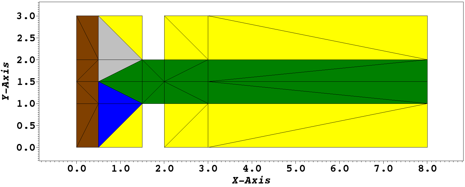
Figure 5: Reference computational domain with subdomains $\Omega_{1}$ (green), $\Omega_{2}$ (yellow), $\Omega_{3}$ (blue), $\Omega_{4}$ (grey) and $\Omega_{5}$ (brown).

For each subdomain $\hat{\Omega}_{k}$ the elemental basis function evaluations are transformed to the reference domain. For each velocity basis function $\mathbf{u}=(u_{1},u_{2}),\mathbf{v}=(v_{1},v_{2}),\mathbf{w}=(w_{1},w_{2})$ and each (scalar) pressure basis function $\psi$, we can write the transformation with summation convention as:

$$\int_{\hat{\Omega}_{k}}\frac{\partial\hat{\mathbf{u}}}{\partial\hat{x}_{i}}\hat{\nu}_{ij}\frac{\partial\hat{\mathbf{v}}}{\partial\hat{x}_{j}}d\hat{\Omega}_{k} = \int_{\Omega_{k}}\frac{\partial\mathbf{u}}{\partial x_{i}}\nu_{ij}\frac{\partial\mathbf{v}}{\partial x_{j}}d\Omega_{k},$$

$$\int_{\hat{\Omega}_{k}}\hat{\psi}\nabla\cdot\hat{\mathbf{u}}d\hat{\Omega}_{k} = \int_{\Omega_{k}}\psi\chi_{ij}\frac{\partial u_{j}}{\partial x_{i}}d\Omega_{k},$$

$$\int_{\hat{\Omega}_{k}}(\hat{\mathbf{u}}\cdot\nabla)\hat{\mathbf{v}}\cdot\hat{\mathbf{w}}d\hat{\Omega}_{k} = \int_{\Omega_{k}}u_{i}\pi_{ij}\frac{\partial v_{j}}{\partial x_{i}}\mathbf{w}d\Omega_{k},$$

with

$$\nu_{ij} = T_{ii^{\prime}}\hat{\nu}_{i^{\prime}j^{\prime}}T_{jj^{\prime}}\det(T)^{-1},$$

$$\chi_{ij} = \pi_{ij}=T_{ij}\det(T)^{-1}.$$

The subdomain $\Omega_{5}$ (see Fig. 5) is kept constant, so that no interpolation of the inflow profile is necessary. To achieve fast reduced order solves, the offline-online decomposition expands the system matrix as in (11) and computes the parameter independent projections offline, which are stored as small-sized matrices of the order $N\times N$. Since in an Oseen-iteration each matrix is dependent on the previous iterate, the submatrices corresponding to each basis function are assembled and then formed online using the reduced basis coordinate representation of the current iterate. This is the same procedure used for the assembly of the nonlinear term in the Navier-Stokes case Hess:Lassila2014 .

5 Numerical Results

The accuracy of the ROM is assessed using $40$ snapshots sampled uniformly over the parameter domain $[0.1,2.9]$ for the POD and $40$ randomly chosen parameter locations to test the accuracy. Fig. 6 (left) shows the decay of the energy of the POD modes. To reach the typical threshold of $99.99\%$ on the POD energy, it takes $9$ POD modes as RB ansatz functions. Fig. 6 (right) shows the relative $L^{2}(\Omega)$ approximation error of the reduced order model with respect to the full order model up to $6$ digits of accuracy, evaluated at the $40$ randomly chosen verification parameter locations. With $9$ POD modes the maximum approximation error is less than $0.7\%$ and the mean approximation error is less than $0.5\%$.

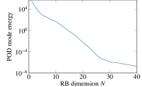
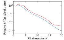
Figure 6: Left: Decay of POD mode energy. Right: Maximum (red) and mean (blue) relative $L^{2}(\Omega)$ error for the velocity over increasing reduced basis dimension.

While the full-order solves were computed with Nektar++, the reduced-order computations were done in ITHACA-SEM with a separate python code. To assess the computational gain, the time for a fixed point iteration step using the full-order system is compared to the time for a fixed point iteration step of the ROM with dimension $20$, both done in python. The ROM online phase reduces the computational time by a factor of over $100$. The offline time is dominated by computing the snapshots and the trilinear forms used to project the advection terms. See Hess:Lassila2014 for detailed explanations.

6 Conclusion and Outlook

We showed that the POD reduced basis technique generates accurate reduced order models for SEM discretized models under parametric variation of the geometry. The potential of a high-order spectral element method with a reduced basis ROM is the subject of current investigations. See also Hess:Taddei . Since each spectral element comprises a block in the system matrix in local coordinates, a variant of the reduced basis element method (RBEM) (Hess:Maday2002195 ; Hess:lovgren_maday_ronquist_2006 ) can be successfully applied in the future.

References

- (1) Karniadakis, G., Sherwin, S.: Spectral/hp Element Methods for Computational Fluid Dynamics. In: Oxford University Press, 2nd ed. (2005).
- (2) Canuto, C., Hussaini, M.Y., Quarteroni, A., Zhang, Th.A.: Spectral Methods Fundamentals in Single Domains. In: Springer – Scientific Computation, (2006).
- (3) Canuto, C., Hussaini, M.Y., Quarteroni, A., Zhang, Th.A.: Spectral Methods Evolution to Complex Geometries and Applications to Fluid Dynamics. In: Springer – Scientific Computation, (2007).
- (4) Patera, A.T.: A Spectral Element Method for Fluid Dynamics; Laminar Flow in a Channel Expansion. Journal of Computational Physics, 54:3 (1984), 468–488.
- (5) Herrero, H., Maday, Y., Pla, F.: RB (Reduced Basis) for RB (Rayleigh–Bénard). Computer Methods in Applied Mechanics and Engineering, 261–262, (2013), 132–141.
- (6) Fick, L., Maday, Y., Patera A., Taddei T.: A stabilized POD model for turbulent flows over a range of Reynolds numbers: Optimal parameter sampling and constrained projection. Journal of Computational Physics, 371 (2018), 214–243.
- (7) Cantwell, C.D., Moxey, D. , Comerford, A., Bolis, A., Rocco, G., Mengaldo, G., de Grazia, D., Yakovlev, S., Lombard, J.-E., Ekelschot, D., Jordi, B., Xu, H., Mohamied, Y., Eskilsson, C., Nelson, B., Vos, P., Biotto, C., Kirby, R.M., Sherwin, S.J.: Nektar++: An open-source spectral/hp element framework. Computer Physics Communications, 192, (2015), 205–219.
- (8) Holmes, P., Lumley, J., Berkooz, G.: Turbulence, Coherent Structures, Dynamical Systems and Symmetry. Cambridge University Press, (1996).
- (9) Pitton, G., Quaini, A., Rozza, G.: Computational Reduction Strategies for the Detection of Steady Bifurcations in Incompressible Fluid-Dynamics: Applications to Coanda Effect in Cardiology. Journal of Computational Physics, 344, (2017), 534–557.
- (10) Hesthaven, J.S., Rozza, G., Stamm, B.: Certified Reduced Basis Methods for Parametrized Partial Differential Equations. In: SpringerBriefs in Mathematics, (2016).
- (11) Burger, M.: Numerical Methods for Incompressible Flow, Lecture Notes. UCLA (2010).
- (12) Boffi, D., Brezzi F., Fortin, M.: Mixed Finite Element Methods and Applications. Springer Series in Computational Mathematics, (2013).
- (13) Quarteroni, A., Valli, A.: Numerical Approximation of Partial Differential Equations. Springer-Verlag, Berlin-Heidelberg, (1994).
- (14) Pitton, G., Rozza, G.: On the Application of Reduced Basis Methods to Bifurcation Problems in Incompressible Fluid Dynamics. Journal of Scientific Computing, (2017).
- (15) Wille, R., Fernholz, H.: Report on the first European Mechanics Colloquium, on the Coanda effect. Journal of Fluid Mechanics, 23:4 (1965), 801–819.
- (16) Rozza, G.: Real-time reduced basis solutions for Navier-Stokes equations: optimization of parametrized bypass configurations. ECCOMAS CFD 2006 Proceedings on CD, 676 (2006), 1–16.
- (17) Quarteroni, A., Rozza, G.: Numerical Solution of parametrized Navier-Stokes equations by reduced basis methods. Num. Meth. Part. Diff. Eq., 23(4) (2007), 923–948.
- (18) Lassila, T., Manzoni, A., Quarteroni, A., Rozza, G.: Model Order Reduction in Fluid Dynamics: Challenges and Perspectives. In: Reduced Order Methods for Modelling and Computational Reduction, Springer International Publishing, MS&A, Vol. 9, A. Quarteroni, G.Rozza eds. (2014), 235–273.
- (19) Maday, Y., Ronquist, E.M.: A Reduced-Basis Element Method. Comptes Rendus Mathematique 335:2 (2002), 195–200.
- (20) Lovgren, A.E., Maday, Y, Ronquist, E.M.: A Reduced Basis Element Method for the Steady Stokes Problem. ESAIM: Mathematical Modelling and Numerical Analysis 40:3 (2006), 529–552.
- (21) Hess, M.W., Rozza, G.: A Spectral Element Reduced Basis Method in Parametric CFD. Numerical Mathematics and Advanced Applications - ENUMATH 2017, Springer, in press, ArXiv e-print 1712.06432, (2018).
- (22) Hess, M.W., Alla, A., Quaini, A., Rozza, G., Gunzburger, M.: A Localized Reduced-Order Modeling Approach for PDEs with Bifurcating Solutions. ArXiv e-print 1807.08851, accepted for publication in Computer Methods in Applied Mechanics and Engineering (CMAME), (2019).