An effective clustering method based on data indeterminacy in neutrosophic set domain

Abstract

In this work, a new clustering algorithm is proposed based on neutrosophic set (NS) theory. The main contribution is to use NS to handle boundary and outlier points as challenging points of clustering methods. In the first step, a new definition of data indeterminacy (indeterminacy set) is proposed in NS domain based on density properties of data. Lower indeterminacy is assigned to data points in dense regions and vice versa. In the second step, indeterminacy set is presented for a proposed cost function in NS domain by considering a set of main clusters and a noisy cluster. In the proposed cost function, two conditions based on distance from cluster centers and value of indeterminacy, are considered for each data point. In the third step, the proposed cost function is minimized by gradient descend methods. Data points are clustered based on their membership degrees. Outlier points are assigned to noise cluster; and boundary points are assigned to main clusters with almost same membership degrees. To show the effectiveness of the proposed method, three types of datasets including diamond, UCI and image datasets are used. Results demonstrate that the proposed cost function handles boundary and outlier points with more accurate membership degrees and outperforms existing state of the art clustering methods in all datasets.

1 Introduction

Clustering is a division of data into groups. Each group, referred as a cluster, attempts to satisfy two rules: objects are similar (or related) to each other (minimize the intra-cluster distance) inside same groups and at the same time different from (or unrelated to) the other groups (maximize the inter-cluster distance) . Clustering represents and models data by few clusters which achieves simplification to data analysis. Data clustering is an important field in machine learning, and has found numerous applications in computer vision, image processing, taxonomy, medicine, geology, business, and pattern recognition community [1, 2, 3, 4, 5].

In data analysis, clustering methods can be considered as two popular categories: hard (crisp) and fuzzy methods [6]. In hard clustering methods, data points are grouped so that each one belongs to exactly one cluster. Unlike hard clustering, in fuzzy partitioning, each object may be assigned to all clusters with different degrees of membership [7]. One of the most popular hard clustering methods is K-means which partitions the data into k clusters automatically attempting to minimize the within-group sum of square distances [8]. The main disadvantage of this algorithm is that it does not ensure a global minimum of variance and needs a predefined cluster numbers [9]. K-means++ is an improvement of clustering analysis on k-means [10]. It improves the k-means with choosing the initial cluster values (or ”seeds”). It was proposed as an approximation algorithm for the NP-hard k-means problem. K-medoids is also a variation of k-means where it calculates the median for each cluster to determine its centroid. It has the effect of minimizing error over all clusters with respect to the 1-norm distance metric, which relates directly to the k-means algorithm. The Euclidean distance between points is considered as a criterion for clustering and a point designated as the center of that cluster.

Fuzzy c-means (FCM) clustering is one of the most popular fuzzy methods. FCM allows one point of data to belong to two or more clusters with different membership degrees [11]. FCM was developed by Dunn in [12] and improved by Bezdek [13]. FCM has four major problems: 1. It just attempts to minimize intra-cluster variance as well, but does not consider the inter-cluster variance, like k-means algorithm. 2. The result of clustering strongly depends on initializing. 3. It sensitives to noise and the membership of noise points can be high. 4. It is also sensitive to the type of distance metric and cannot distinguish between equally highly likely and equally highly unlikely data points [14, 15, 16]. To solve the last problem, Gustafson and Kessel considered the Mahalanobis distance to show the shape effect on distance metric [17]. In [18], a new method based on possibility named as possibilistic c-means (PCM) was proposed. However, it is sensitive to cluster center initialization, and needs tuning additional parameters, and may lead to generate coincident clusters. To overcome PCM problems, Pal et al. combined PCM and FCM where both the relative and absolute resemblances are considered for cluster centers [19]. In [20], fuzzy non-metric model (FNM) was proposed as a clustering approach. Richards et al. presented a variation of fuzzy and hard clustering named as relational fuzzy c-means (RFCM) [21]. In [22], Dave combined FNM and RFCM which was robust against noise and outliers. More recent researches for fuzzy c-means are evidential c-means (ECM) [23] and relational evidential c-means (RECM) [24]. Recently, many clustering methods have been developed based on different theories [25, 26, 27, 28, 29].

Neutrosophy theory was firstly proposed by Smarandache in 1995 [30]. It is a branch of philosophy, and studies the origin, nature and scope of neutralities, as well as their interactions with different ideational spectra [31]. This theory was applied for image processing first by Guo et. al [32] and then it has been successfully used for other image processing domains including image segmentation [33, 32, 34, 35, 36, 37], image thresholding [38], image edge detection [39], image retrieval [40, 41], retinal image analysis [42, 43, 44, 45, 46, 47, 48], liver image analysis[49, 50], breast ultrasound image analysis[51], data classification[52] and uncertainty handling[53]. Recently, NS has been adapted for our problem of interest, data and image clustering, as neutrosophic c-means (NCM) [7] and kernel neutrosophic c-means (KNCM) [54].

The main motivation of this work is to handle boundary and outlier points by proposing indeterminacy set(I) in NS domain followed by presenting this set for a new clustering cost function. As it will be discussed in section 4 and 5, challenges of the previous methods are addressed by encoding all constraints for handling boundary and outlier points in the cost function. In this paper, we introduce a new method based on neutrosophic set (NS) theory for data clustering and image segmentation. It calculates the indeterminacy for each data point in NS domain followed by a new cost function based on data indeterminacy. In the proposed cost function two conditions for data point i are considered to have the highest membership degree to the main cluster k: (a) point i should have the minimum distance from the cluster center k rather than other clusters, (b) point i should have a small indeterminacy. Similarly, there are also two conditions for point i to have the highest membership degree to noisy cluster: (a) having the maximum sum distance from all main clusters and (b) having a big indeterminacy. In the third step, the proposed cost function is minimized by gradient descend methods. Data points are clustered based on their membership degrees. Outlier points are assigned to noise cluster; and boundary points are assigned to main clusters with almost same membership degrees. The proposed cost function is minimized and assigns membership degrees to main and noise clusters. Here, membership sets T and F in NS domain are considered as the main and noisy clusters, respectively. The rest of the paper is organized as follows. FCM algorithm and NS set are reviewed in section 2. In section 3, the proposed method is presented. Experimental results of the proposed method in scatter and image datasets are illustrated in Section 4. Section 5 discusses advantages and disadvantages of the proposed method in comparison with other methods. Finally, section 6 concludes the paper.

2 Review on neutrosophic set and fuzzy clustering

The proposed methods in this paper are based on NS and fuzzy clustering. In this section, these concepts are introduced as follows.

2.1 Neutrosophic set

NS is a powerful framework of neutrosophy in which neutrosophic operations are defined from a technical point of view. In fact, for each application, neutrosophic sets are defined as well as neutrosophic operations corresponding to that application. Generally, in neutrosophic set $A$, each member $x$ in $A$ is denoted by three real subsets true, false and indeterminacy in interval $[0,1]$ referred as $T$, $F$ and $I$, respectively. Each element is expressed as $x(t,i,f)$ which means that it is $t$% true, $i$% indeterminacy, and $f$% false. In each application, domain experts propose the concepts behind true, false and indeterminacy[32].

2.2 Fuzzy clustering

Clustering methods can classify similar samples into the same group. Consider $X$ be a data set, and xi be a sample. The purpose of clustering is to find partitions $C=\{C_{1},C_{2},...,C_{m}\},$ which satisfies (1):

$$X=\sum_{i=1}^{m}C_{i}\ ,C_{i}\neq\emptyset\ for(i=1,2,…,m),C_{i}\cap C_{j}=\emptyset\ for(i,j=1,2,…,m);i\neq j$$ (1)

FCM attempts to cluster a limited number of elements $X=\{X_{1},X_{2},...,X_{n}\},$ into a collection of c fuzzy clusters based on the similar features. Given a finite set of data, the FCM returns a list of c cluster centers $C=\{C_{1},C_{2},...,C_{c}\},$ and a partition matrix $W=\{w_{i,j}|w_{i,j}\in[0,1],i=1,2,...,n,j=1,2,...,c\}$ where $w_{i,j}$ represents the membership degree of data point $x_{i}$ to cluster $c_{j}$.

The FCM aims to minimize objective function in (2):

$$J=argmin\sum_{i=1}^{n}\sum_{j=1}^{c}||X_{i}-C_{j}||^{2}$$ (2)

where membership degrees $w_{i,j}$ and cluster centers $c_{j}$ are updated in each iteration by (3)-(4):

$$w_{i,j}=\dfrac{1}{\sum_{j=1}^{c}(\dfrac{||X_{i}-C_{j}||}{||X_{i}-C_{j}||})^{2/(m-1)}}$$ (3)

$$c_{k}=\dfrac{\sum_{x}w_{k}(x^{m})x}{\sum_{x}w_{k}(x^{m})}$$ (4)

The iteration will not stop until max $\{|w_{i,j}^{(k+1)}-w_{i,j}^{(k)}|\}\leqslant\varepsilon$ where $\varepsilon$ is a small quantity and $k$ is the iteration step. This procedure attempts to achieve a minimum or a saddle point of $j$. Each data is assigned into all classes with different membership degrees[55].

3 Proposed method

In this paper, a new clustering approach is proposed to cluster data including outlier and boundary data points. The proposed method is derived from FCM and NS concepts. Here, uncertainty is defined for each data point and described using the indeterminacy set in neutrosophic domain. Indeterminacy value for each data point i is defined by considering the Euclidean distance of i from its neighbors by (5)-(7).

$$I(i)=\begin{cases}1-\dfrac{NP(i)}{N/NC},&\text{if }NP(i)<NP_{th}\\ \alpha,&\text{otherwise}\end{cases}$$ (5)

$$temp[j]=\begin{cases}1,&\text{if }dist[i,j]<Eps,j=1,2,...,N\\ 0,&\text{otherwise}\end{cases}$$ (6)

$$NP(i)=\sum_{j=1}^{N}temp[j]$$ (7)

where $I$ is an indeterminacy value, $N$ is the size of dataset, $NC$ is the number of clusters and $NP_{th}$ is a constant number as a threshold value. For indeterminacy assessment, the value of $NP_{i}$ is compared with $NP_{th}$. If $NP$ is smaller than $NP_{th}$, it means that this point is a noisy point and should have a bigger indeterminacy. Otherwise, small quantity $Eps$ is considered for indeterminacy. $dist[i,j]$ is the Euclidean distance between point $i$ and $j$. It is clear that this idea assigns indeterminacy near to $1$ for noisy pixels and near to $0$ for points inside the main clusters.

In the proposed clustering algorithm, we consider both determinate and indeterminate membership degrees for main clusters and noisy cluster, respectively. A unique set $A$ has been considered as a union of determinate and indeterminate clusters. Let $A=C_{i}\cup R;i=1,2,...,k$; where $C_{i}$ and $R$ represents determinate cluster $i$ and indeterminate cluster, respectuvely. $\cup$ is the union operation. Considering indeterminacy in clustering, the proposed objective function is defined in (8):

$$L(T,F,C)=\sum_{i=1}^{n}\sum_{j=1}^{k}(w_{1}I_{i}T_{i,j})^{m}||X_{i}-C_{j}||^{2}+\sum_{j=1}^{k}(w_{2}(1-I_{i})F_{i})^{m}(k-||X_{i}-C_{j}||^{2})$$ (8)

where $k$ is the number of clusters. $T_{i,j}$ and $F_{i}$ are the membership degrees of data point $i$ to main cluster $j$ and noisy cluster, respectively. To consider constraints in NS theory, membership degrees are enforced to be in interval $0<T_{i,j},F_{i}<1$. For each data point, the sum of $T_{i,j}$ and $F_{i}$ should be equal to $1$ which is satisfied as following:

$$\sum_{j=1}^{k}T_{i,j}+F_{i}=1$$ (9)

We consider two conditions for data point $i$ to have the highest membership degree to cluster $k$: $(a)$ point $i$ should have the minimum distance from the cluster center $k$ rather than other clusters, $(b)$ point $i$ should have a small indeterminacy. Similarly, there are also two conditions for point $i$ to have the highest membership degree to noisy cluster: $(a)$ having the maximum sum distance from all main clusters $\sum_{j=1}^{k}||X_{i}-C_{j}||^{2}$ and $(b)$ having a big indeterminacy. The maximum difference between any two pixels is $1$ since all sets have been normalized to the interval $[0,1]$. Therefore, the maximum quantity for $\sum_{j=1}^{k}||X_{i}-C_{j}||^{2}$ is $k$.

For considering this constraint, the Lagrange function is constructed by (10):

$$\begin{split}L(T,F,C)=\sum_{i=1}^{n}\sum_{j=1}^{k}(w_{1}I_{i}T_{i,j})^{m}||X_{i}-C_{j}||^{2}+\sum_{j=1}^{k}(w_{2}(1-I_{i})F_{i})^{m}(k-||X_{i}-C_{j}||^{2})\\ -\sum_{i=1}^{n}\lambda_{i}(\sum_{j=1}^{k}T_{i,j}+F_{i}-1)\end{split}$$ (10)

For cost function minimization, gradient descent approach is used. Therefore:

$$\dfrac{\partial L}{\partial T_{ij}}=m(w_{1}I_{i}T_{ij})^{(m-1)}||X_{i}-C_{j}||^{2}-\lambda_{i}$$ (11)

$$\dfrac{\partial L}{\partial F_{i}}=m(w_{2}(1-I_{i})F_{i})^{(m-1)}(K-||X_{i}-C_{j}||^{2})-\lambda_{i}$$ (12)

$$\dfrac{\partial L}{\partial C_{j}}=-(w_{1}I_{i}T_{ij})^{m}(X_{i}-C_{j})+(w_{2}(1-I_{i})F_{i})^{m}(X_{i}-C_{j})$$ (13)

By considering $\dfrac{\partial L}{\partial F_{i}}=0$, $\dfrac{\partial L}{\partial F_{i}}=0$ and $\dfrac{\partial L}{\partial C_{j}}=0$ we can obtain the follows:

$$T_{ij}=\dfrac{1}{w_{1}I_{i}}(\dfrac{\lambda_{i}}{m})^{\dfrac{1}{(m-1)}}||X_{ij}-C_{j}||^{\dfrac{-2}{(m-1)}}$$ (14)

$$F_{i}=\dfrac{1}{w_{2}(1-I_{i})}(\dfrac{\lambda_{i}}{m})^{\dfrac{1}{(m-1)}}(K-(||X_{ij}-C_{j}||)^{2})^{\dfrac{-1}{(m-1)}}$$ (15)

$$C_{j}=\dfrac{[\sum_{i=1}^{n}(w_{1}I_{i}T_{ij})^{m}-\sum_{i=1}^{n}(w_{2}(1-I_{i})F_{i})]X_{i}}{\sum_{i=1}^{n}(w_{1}I_{i}T_{ij})^{m}-\sum_{i=1}^{n}(w_{2}(1-I_{i})F_{i})}$$ (16)

For efficient computation, term $(\dfrac{\lambda_{i}}{m})^{\dfrac{1}{m-1}}$ can be assumed as $K_{temp}$ and computed by replacing $T_{ij}$ and $F_{i}$ in (9):

$$(\dfrac{\lambda_{i}}{m})^{\dfrac{1}{m-1}}=K_{temp}$$ (17)

$$\sum_{j=1}^{k}\dfrac{K_{temp}}{w_{1}I_{i}}||X_{ij}-C_{j}||^{\dfrac{-2}{(m-1)}}+\dfrac{K_{t}emp}{w_{2}(1-I_{i})}(K-\sum_{j=1}^{k}||X_{ij}-C_{j}||)^{\dfrac{-1}{(m-1)}}=1$$ (18)

$$K_{temp}=[\dfrac{1}{w_{1}I_{i}}\sum_{j=1}^{k}||X_{ij}-C_{j}||^{\dfrac{-2}{(m-1)}}+\dfrac{1}{w_{2}(1-I_{i})}(K-(\sum_{j=1}^{k}||X_{ij}-C_{j}||^{2}))^{\dfrac{-1}{(m-1)}}]^{-1}$$ (19)

$$T_{ij}=\dfrac{K_{temp}}{w_{1}I_{i}}||X_{ij}-C_{j}||^{\dfrac{-2}{(m-1)}}$$ (20)

$$F_{i}=\dfrac{K_{temp}}{w_{2}(1-I_{i})}(K-(\sum_{j=1}^{k}||X_{ij}-C_{j}||^{2}))^{\dfrac{-1}{(m-1)}}$$ (21)

The proposed clustering algorithm is summarized as follows:

Algorithm 1

1:Initialize $T$ and $F$.

2:Initialize the $c$, $w1$, $w2$, $Eps$, $K$ and $m$.

3:Compute $I$ for each data point.

4:Update $T_{ij}$, $F_{i}$ and $C_{i}$ by Eqs (20), (21) and (16), respectively.

5:Check the stop condition, if $|T^{(k)}-T^{(k-1)}|<\varepsilon$ then stop, otherwise go to $step$ $4$.

6:Assign each data point into boundary cluster if the first two membership degrees $T_{ij}$ and $T_{ik}$ are between $t$ and $(1-t)$, otherwise assign it to a cluster which data point $i$ has the maximum membership degree to it.

7:end.

4 Experimental Results

Performance of the proposed clustering method is evaluated in three types of datasets including diamond datasets, natural and artificial images datasets and medical image dataset in sections 4.1, 4.2 and 4.3, respectively. The proposed method is applied on these datasets and then compared with ASIC [56], FCM-AWA [57], NCM [7] and methods in [42, 43, 58, 59, 60, 61, 62].

4.1 Parameters Tuning

All parameters in indeterminacy computation section are set to following quantities based on experiments. Parameter $Eps$ and $NP_{th}$ are considered with quantity $4$, means that neighbors in the maximum distance of $4$ and the maximum of $4$ neighbors are considered for indeterminacy computation. Parameter $\alpha$ is considered with quantity $0.05$. In the proposed cost function, parameter are configured as $\varepsilon=10^{-6}$, $m=2$, $t=0.4$, $w_{1}=1$ and $w_{2}=2$.

4.2 Datasets

In this research, three type of datasets are used to evaluate the performance of the proposed method. The first type is diamond datasets including a collections of scatter data including X12, X19 and X24 which are proposed in [7]. We also proposed X35 which is an extension of datasets in [7]. In these datasets, boundary points are considered between main clusters as well as outlier points far from main clusters. It can be visually seen that how clustering methods are affected by these points among main points in each dataset. The second dataset type is UCI which include datasets with higher dimension and larger scale. Here, ”Iris”, ”Wine”, ”Glass”, ”Seeds” and ”Breast-w” are used. Finally, the proposed method is applied on image data as third dataset type. In this experiment, these dataset natural, artificial and medical images are used to evaluate the effectiveness of the proposed method.

4.3 Diamond datasets

Diamond datasets in NCM including: $a)$ $X12:12$ scatter points in $2$ clusters with $1$ boundary point and $1$ outlier, $b)$ $X19:19$ scatter points in $3$ clusters with $2$ boundary points and $2$ outliers and $c)$ $X24:24$ scatter points in $4$ clusters with $3$ boundary points and $1$ outlier were used in this research. We also designed a further scatter dataset referred as $X35$.

4.3.1 X12 dataset

$X12$ is shown in Fig. 1 in which points $1-5$ and $7-11$ belong to main clusters, points $6$ and $12$ are boundary and outlier, respectively. In all experiments, $T_{ci}$ is the membership degree to $i_{th}$ cluster and $F$ represents the membership degree to noise cluster. Each data point is assigned to a cluster with the maximum membership degree. Fig. 2 illustrates assigned membership degrees of each point to two main clusters and noisy cluster by the proposed method with $red$, $green$ and $blue$ colors, respectively. Table 1 reports the membership degrees assigned by the proposed clustering method and NCM. Although, both the proposed method and NCM assign correct cluster labels to all points, the proposed method determines the cluster labels more confidently. For example, for point $7$ which is a point in cluster $2$, the proposed method assigns $0.91$ membership degree to this cluster while NCM assigns $0.69$. All membership degreess are also visually depicted in Fig. 3 . Dash $("-.-.-")$ and circle $("o-o-o")$ represent membership degrees computed by NCM and the proposed method, respectively.

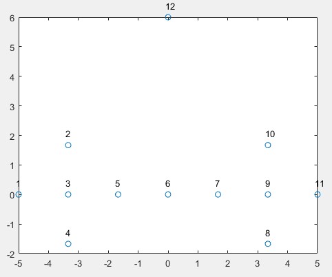
Figure 1: X12 dataset.

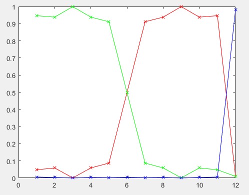
Figure 2: Membership degrees for X12 dataset computed by the proposed method.

Table 1: Clustering result for X12 dataset.

	NCM				Proposed method
	Tc1	Tc2	I	F	Tc1	Tc2	F
1	0.8262	0.0294	0.0104	0.1339	0.9515	0.0479	0.0006
2	0.7952	0.0451	0.0196	0.1401	0.9409	0.0588	0.0003
3	0.9996	0.0001	0.0000	0.0003	0.9993	0.0007	0.0000
4	0.792	0.0456	0.0197	0.1426	0.9409	0.0588	0.0003
5	0.695	0.0799	0.0915	0.1336	0.9124	0.0874	0.0002
6	0.0007	0.0007	0.9982	0.0005	0.4998	0.4998	0.0004	boundary
7	0.0835	0.6802	0.0990	0.1373	0.0874	0.9124	0.0002
8	0.0475	0.7854	0.0207	0.1464	0.0588	0.9409	0.0003
9	0.0003	0.9987	0.0001	0.0008	0.0007	0.9993	0.0000
10	0.0444	0.7994	0.0195	0.1367	0.0588	0.9409	0.0003
11	0.0284	0.8334	0.0101	0.128	0.0479	0.9515	0.0006
12	0.0477	0.0938	0.0084	0.8502	0.0765	0.0765	0.847

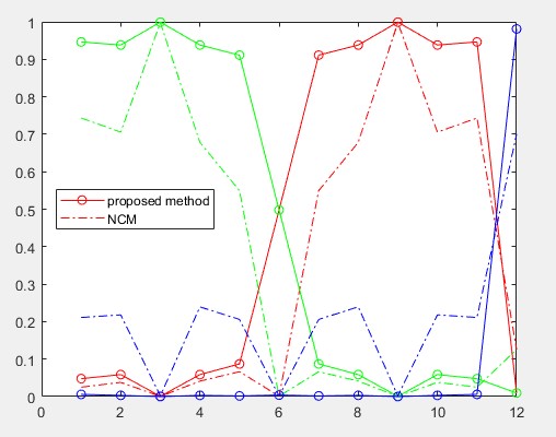
Figure 3: Membership degrees computed by NCM and the proposed method in X12.

4.3.2 X19 datasets

$X19$ dataset with three clusters is shown in Fig. 4 . In this dataset, points $1-5$, $7-11$ and $13-17$ represent main clusters, points $6$ and $12$ are boundary and points $18$ and $19$ are noisy points. Membership degrees computed by the proposed method and NCM are reported in Table 2 . Similar to section $4.2.1$, although the proposed method and NCM assign same cluster labels for all points, the proposed method assigns membership degrees for points such as $5$, $7$, $11$, $12$ with higher certainties into their corresponding clusters. Point $6$ belongs to boundary cluster and point $3$ is a main cluster center. Although, point $5$ has a same distance between main and boundary clusters, it belongs to main cluster. NCM cannot distinguish boundary and main clusters for point $5$. The proposed method addresses this issue and assigns $0.91$ of membership degree to main cluster while NCM assigns $0.58$. Fig. 5 depicts membership degrees visually.

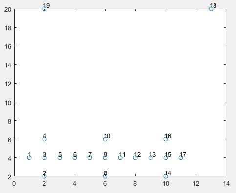
Figure 4: X19 dataset.

Table 2: Clustering result for X19 dataset.

	NCM					Proposed method
	Tc1	Tc2	Tc3	I	F	T1	T2	T3	F
1	0.89	0.0236	0.007	0.015	0.0645	0.0169	0.9307	0.0525	0
2	0.7759	0.0578	0.0144	0.0444	0.1076	0.0491	0.7913	0.1596	0
3	0.988	0.003	0.0007	0.0029	0.0053	0.0006	0.9972	0.0022	0
4	0.8393	0.0411	0.0103	0.0332	0.0762	0.0491	0.7913	0.1596	0
5	0.5816	0.0928	0.0161	0.2182	0.0913	0.0131	0.9194	0.0675	0
6	0.0124	0.0149	0.0016	0.9646	0.0065	0.0507	0.5211	0.4282	0	boundary
7	0.0689	0.7032	0.0261	0.1249	0.0769	0.0369	0.1081	0.855	0
8	0.0434	0.792	0.0434	0.0317	0.0894	0.1507	0.1507	0.6985	0
9	0	0.9999	0	0	0	0	0	1	0
10	0.0421	0.7996	0.0421	0.0315	0.0847	0.1507	0.1507	0.6985	0
11	0.0261	0.7032	0.0689	0.1249	0.0769	0.1081	0.0369	0.855	0
12	0.0016	0.0149	0.0124	0.9646	0.0065	0.5211	0.0507	0.4282	0	boundary
13	0.0161	0.0928	0.5816	0.2182	0.0913	0.9194	0.0131	0.0675	0
14	0.0144	0.0578	0.7759	0.0444	0.1076	0.7913	0.0491	0.1596	0
15	0.0007	0.003	0.988	0.0029	0.0053	0.9972	0.0006	0.0022	0
16	0.0103	0.0411	0.8393	0.0332	0.0762	0.7913	0.0491	0.1596	0
17	0.007	0.0236	0.89	0.015	0.0645	0.9307	0.0169	0.0525	0
18	0.037	0.0854	0.3046	0.0324	0.5406	0.0458	0.0327	0.0399	0.8817
19	0.3046	0.0854	0.037	0.0324	0.5406	0.0616	0.0763	0.0718	0.7904

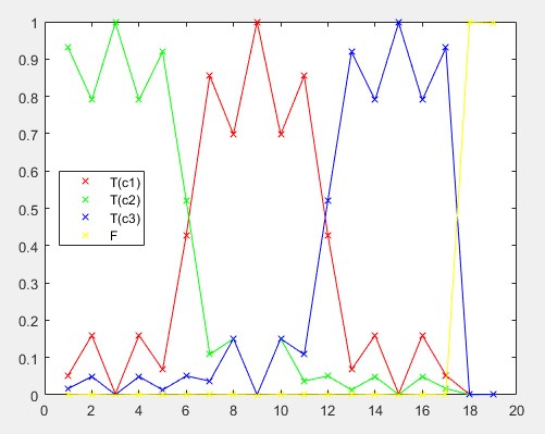
Figure 5: Membership degrees computed by the proposed method in X19.

4.3.3 X24 dataset

We also conducted more experiment to compare the proposed method and NCM using a four class dataset $X24$ which is represented in Fig. 6 . Data points $6$, $12$ and $18$ are boundary and $24$ is an outlier. The results of the proposed method and NCM are tabulated in Table 3 . The first five data points belong to the first main cluster because of their higher $T_{c1}$ values. Similar observation can be inferred for the other clusters ($C2$ and $C3$ and $C4$). Data points $6$, $12$ and $18$ are ambiguous because of the two highest $T$ values. Finally, last data point $(24)$ is deduced as outlier. Fig. 7 depicts membership degrees visually.

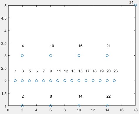
Figure 6: X24 dataset.

Table 3: Clustering result for X24 dataset.

	NCM						Proposed method
	Tc1	Tc2	Tc3	Tc4	I	F	Tc1	Tc2	Tc3	Tc4	F
1	0.0248	0.0075	0.8631	0.0035	0.0363	0.0648	0.0459	0.0069	0.9322	0.0143	0.0006
2	0.0464	0.0119	0.77	0.0052	0.0839	0.0825	0.0547	0.0066	0.9238	0.0144	0.0004
3	0.0015	0.0004	0.9925	0.0002	0.0031	0.0024	0.0008	0.0001	0.9989	0.0002	0
4	0.0464	0.0119	0.7703	0.0052	0.0839	0.0824	0.0547	0.0066	0.9238	0.0144	0.0004
5	0.0703	0.0126	0.4752	0.005	0.3709	0.0661	0.0782	0.006	0.901	0.0145	0.0003
6	0.003	0.0003	0.0026	0.0001	0.9928	0.0012	0.4364	0.0181	0.4957	0.0492	0.0007	boundary
7	0.5937	0.023	0.0595	0.0069	0.255	0.0619	0.8495	0.011	0.1043	0.0349	0.0003
8	0.7527	0.0428	0.0414	0.0108	0.0732	0.0791	0.8792	0.0139	0.0546	0.052	0.0003
9	1	0	0	0	0	0	1	0	0	0	0
10	0.7537	0.0427	0.0412	0.0108	0.073	0.0786	0.8792	0.0139	0.0546	0.052	0.0003
11	0.5769	0.0611	0.0218	0.0109	0.2687	0.0606	0.8538	0.0176	0.0349	0.0934	0.0003
12	0.0007	0.0007	0.0001	0.0001	0.9981	0.0003	0.4485	0.0512	0.0512	0.4485	0.0006	boundary
13	0.0663	0.5152	0.0117	0.0215	0.3228	0.0626	0.0934	0.0349	0.0176	0.8538	0.0003
14	0.0449	0.7462	0.0113	0.0392	0.0785	0.0799	0.052	0.0546	0.0139	0.8792	0.0003
15	0.0004	0.9978	0.0001	0.0003	0.0008	0.0006	0	0	0	1	0
16	0.0437	0.7518	0.011	0.0389	0.0768	0.0778	0.052	0.0546	0.0139	0.8792	0.0003
17	0.0224	0.6581	0.0067	0.0522	0.202	0.0587	0.0349	0.1043	0.011	0.8495	0.0003
18	0.0018	0.0174	0.0006	0.0124	0.9611	0.0067	0.0492	0.4957	0.0181	0.4364	0.0007	boundary
19	0.0128	0.0733	0.005	0.3824	0.461	0.0655	0.0145	0.901	0.006	0.0782	0.0003
20	0.0013	0.0053	0.0006	0.9722	0.0122	0.0085	0.0002	0.9989	0.0001	0.0008	0
21	0.011	0.0438	0.0048	0.7807	0.0846	0.075	0.0144	0.9238	0.0066	0.0547	0.0004
22	0.014	0.0553	0.0061	0.7268	0.1028	0.095	0.0144	0.9238	0.0066	0.0547	0.0004
23	0.0058	0.0195	0.0027	0.8928	0.0297	0.0495	0.0143	0.9322	0.0069	0.0459	0.0006
24	0.0353	0.0753	0.02	0.2413	0.0633	0.5649	0.0087	0.0515	0.0051	0.0182	0.9165

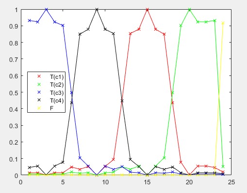
Figure 7: Membership degrees computed by the proposed method in X24.

4.3.4 X35 dataset

We also evaluated the proposed method for our diamond dataset with $35$ data points which is shown in Fig. 8 . Points $1-9$, $13-21$ and $25-33$ belong to main clusters, points $10-12$ and $22-24$ are ambiguous and points $34$ and $35$ are outliers. In this dataset, we have considered more ambiguous points to see the effect of boundary points in final clustering results. Table 4 reports membership degrees computed by the proposed method and NCM. In NCM, points $(3,6,9)$, $(13,16,19)$, $(15,18,21)$ and $(25,28,31)$ are assigned to main clusters with almost $0.50$ membership degree, while in the proposed method, these points are assigned to main clusters with membership degree between $0.80$ to $0.90$. In fact, the proposed clustering scheme can solve the clustering problems in boundary points more efficiently. The membership degrees for each data point are visually depicted in Fig. 9 .

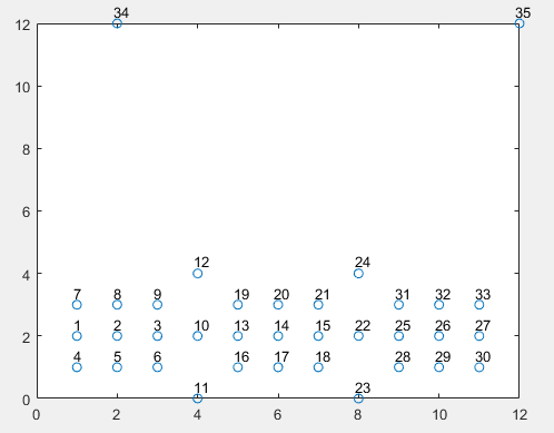
Figure 8: X35 dataset.

Table 4: Clustering result for X35 dataset.

	NCM					Proposed method
	Tc1	Tc2	Tc3	I	F	Tc1	Tc2	Tc3	F
1	0.0069	0.0234	0.8738	0.0346	0.0612	0.0175	0.0541	0.9271	0.0013
2	0.0005	0.0021	0.9894	0.0046	0.0035	0.0007	0.0027	0.9965	0
3	0.0125	0.0714	0.46	0.3888	0.0673	0.0125	0.0643	0.9227	0.0005
4	0.0148	0.0485	0.738	0.0664	0.1323	0.0278	0.0839	0.8862	0.0021
5	0.0121	0.0483	0.7656	0.0878	0.0862	0.0157	0.0569	0.9266	0.0009
6	0.0211	0.1106	0.4555	0.2965	0.1163	0.0288	0.1357	0.8343	0.0011
7	0.0142	0.0469	0.7471	0.0646	0.1272	0.0278	0.0839	0.8862	0.0021
8	0.0114	0.0455	0.7785	0.0839	0.0807	0.0157	0.0569	0.9266	0.0009
9	0.0205	0.1081	0.4566	0.3023	0.1125	0.0288	0.1357	0.8343	0.0011
10	0.0005	0.0044	0.0037	0.9896	0.0018	0.0503	0.4223	0.5261	0.0013	boundary
11	0.0485	0.2536	0.2324	0.2504	0.2151	0.0915	0.4294	0.4764	0.0028	boundary
12	0.0476	0.2543	0.2314	0.2565	0.2101	0.0915	0.4294	0.4764	0.0028	boundary
13	0.0224	0.6022	0.0595	0.2528	0.063	0.0371	0.8528	0.1094	0.0006
14	0	0.9998	0	0.0001	0.0001	0	1	0	0
15	0.0595	0.6023	0.0225	0.2527	0.0631	0.1095	0.8527	0.0372	0.0006
16	0.0381	0.5179	0.0952	0.2375	0.1113	0.0636	0.762	0.1733	0.0012
17	0.043	0.7569	0.043	0.0736	0.0835	0.0575	0.8843	0.0575	0.0007
18	0.0951	0.5181	0.0382	0.2372	0.1114	0.1733	0.7619	0.0636	0.0012
19	0.0367	0.5253	0.0923	0.2386	0.107	0.0636	0.762	0.1733	0.0012
20	0.0398	0.7747	0.0398	0.0689	0.0768	0.0575	0.8843	0.0575	0.0007
21	0.0922	0.5253	0.0368	0.2386	0.1071	0.1733	0.7619	0.0636	0.0012
22	0.0038	0.0045	0.0005	0.9894	0.0019	0.5262	0.4221	0.0503	0.0013	boundary
23	0.232	0.2537	0.0486	0.2503	0.2153	0.4764	0.4293	0.0915	0.0028	boundary
24	0.2313	0.2543	0.0476	0.2567	0.2101	0.4764	0.4293	0.0915	0.0028	boundary
25	0.4585	0.0715	0.0125	0.3902	0.0674	0.9228	0.0642	0.0125	0.0005
26	0.9891	0.0021	0.0005	0.0047	0.0036	0.9965	0.0027	0.0007	0
27	0.8745	0.0233	0.0069	0.0344	0.0609	0.927	0.0541	0.0175	0.0013
28	0.4545	0.1107	0.0212	0.297	0.1165	0.8344	0.1357	0.0288	0.0011
29	0.7648	0.0485	0.0122	0.0881	0.0865	0.9266	0.0569	0.0157	0.0009
30	0.7381	0.0485	0.0148	0.0664	0.1322	0.8862	0.0839	0.0278	0.0021
31	0.4561	0.1081	0.0205	0.3029	0.1125	0.8344	0.1357	0.0288	0.0011
32	0.7788	0.0454	0.0113	0.0838	0.0806	0.9266	0.0569	0.0157	0.0009
33	0.748	0.0467	0.0142	0.0644	0.1268	0.8862	0.0839	0.0278	0.0021
34	0.0447	0.0645	0.0748	0.0361	0.7798	0.0024	0.0033	0.0038	0.9906
35	0.0742	0.0563	0.0375	0.0332	0.7987	0.0023	0.0018	0.0012	0.9947

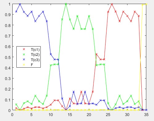
Figure 9: Membership degrees computed by the proposed method in X35.

4.4 UCI Datasets

To show the performance of the proposed method on larger scale datasets, UCI datasets are used. These datasets are considered as standard datasets in machine learning community. In this research, ”Iris”, ”Wine”, ”Glass”, ”Seeds” and ”Breast-w” datasets are selected among other datasets in UCI. Table 5 summaries number of features, number of classes, samples in each cluster and number of objects in each dataset. Accuracy of the proposed method and FCM [63], PCM [64], PFCM [65] and HPFCM [66] methods are summarized in Table 6. The proposed method outperforms other methods in ”Iris”, ”Wine”, ”Glass”, ”Seeds” and Breast-w datasets with the accuracy of 94.66%, 83.14%, 91.58% and 91.90% and 91.41%, respectively.

Table 5: Summary of dataset characteristics:

Dataset	No. of feature	No. of classes	No. each cluster	No. object
Iris	4	3	50,50,50	150
Wine	13	3	48,59,71	178
Glass	9	6	9,29,13,70,17,76	214
Seed	7	3	70,70,70	210
Breast-w	9	2	241,458	699

Table 6: Clustering accuracy for FCM, PCM, PFCM, HPFCM and Proposed method with five datasets: Iris, Wine, Glass, seeds and Breast cancer.

Data sets	FCM	PCM	PFCM	HPFCM	Proposed method
Iris	89.3	66.7	90	92.9	94.66
Wine	68.5	41.5	70	78.9	83.14
Glass	72.1	55.4	82.3	87.6	91.58
Seeds	78.3	69.8	84.3	86.6	91.90
Breast-w	84.3	61.8	86.3	89.1	91.41

4.5 Natural and artificial images datasets

Pixel clustering can be used for image segmentation in which each cluster is considered as a segment. Each pixel’s intensity is used as a one dimensional data for clustering algorithm. This dataset includes natural and artificial images. In this section, we have applied the proposed method to image segmentation and compared with the existing image segmentation algorithms such as NCM, ASIC [56] and FCM–AWA [57].

In the proposed method, membership sets $T$ and $F$ should be post processed so they can be used for pixels clustering [6]. For each pixel, the average of its neighbors is calculated to descend the influence of undesired factors on the final determination of membership sets. Therefore, image clustering process is same with scatter data except final membership of each pixel is calculated by (22)-(23):

$$\overline{T}(i,j)=\dfrac{1}{z^{2}}\sum_{m,n\in S}T(m,n)$$ (22)

$$\overline{F}(i,j)=\dfrac{1}{z^{2}}\sum_{m,n\in S}F(m,n)$$ (23)

where $z$ represents the size of $S$, which has been set to $3$ in this application. Fig. 10 shows two artificial images in which each row contains the segmentation result of different methods for one image. The first row in Fig. 10 is a synthesized image with four classes and the corresponding gray values are $50$ (upper left, UL), $100$ (upper right, UR), $150$ (low left, LL) and $200$ (low right, LR), respectively. Each cluster (sub-image) contains $64\texttimes 64$ pixels. The image is degraded by the Gaussian noise $(\mu=0$, $\sigma=25.5)$. The second row shows another synthesized image that contains three regions: two equal-sized rectangular on a uniform background and corresponding gray values $20$ (upper step), $100$ (lower step) and $255$ (background). Gaussian noise $(\mu=0$, $\sigma=25.5)$ is also added to this image.

It is visually clear from segmentation results that the proposed method archives good homogeneity in the segmented regions in comparison with NCM, ASIC and FCM–AWA. In the proposed method, boundaries of the homogenous regions are smooth and a few number of pixels are misclassified. As it is reported in Table 7 , the proposed method creates $(43,9)$ misclassified pixels in the segmentation of the artidicial images (Image1, Image 2) which outperforms NCM, FCM-AWA and ASIC with (70,15), (418,235) and (144,47) misclassified pixels, respectively. Note that FCM-AWA has been tested by setting parameters: $m=2$, $\alpha=50$, $\varepsilon=10^{-5}$, $r=2$, $k_{0}=0.45$ and $k_{1}=0.65$. In ASIC method, the cooling factor $\alpha$ is set to $0.95$.

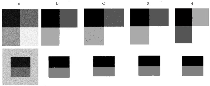
Figure 10: Segmentation results for two samples of artificial images (each sample in one row). (a) original image, semented image by (b) FCM-AWA, (c) ASIC, (d) NCM and (e) the proposed method.

Table 7: Number of misclassified pixels in two artificial images.

	ASIC	FCM-AWA	NCM	Proposed Method
Image 1	144	418	70	43
Image 2	47	235	15	9

We also compared the proposed method with ASIC, FCM-AWA and NCM methods in four natural images: $rice$, $eight$, $Lena$ and $women$ in the first, second, third and forth rows in Fig. 11 , respectively. In these cases, all images are degraded by the Gaussian noise $(\mu=0$, $\sigma=2.25)$. In Fig. 11 , segmentation results of ASIC, FCM– AWA, NCM and the proposed method are depicted in each column.

We further illustrated the proposed method’s performance in image segmentation quantitatively with F-measure [56] which considers both precision (25) and recall (26) of the segmentation results and is defined by (24):

$$F=\dfrac{P.R}{\Psi.P+(1-\Psi).R}$$ (24)

$$P=\dfrac{TP}{TP+FP}$$ (25)

$$R=\dfrac{TP}{TP+FN}$$ (26)

where $\Psi$ is a constant number and is considered as as $0.5$ in [56]. $P$ is precision, and $R$ is recall rate. $TP$ is the number of correct results, $FP$ is the number of false segmented pixels, and $FN$ is the number of the missed pixels in the result. The $F-measure$ value is in the range of $[0,1]$, and a larger $F-Measure$ value indicates a higher segmentation accuracy.

In Table 8 , the $F-measure$ values of each method applied on four natural images are reported. The proposed method achieved the highest F-Measure of 0.93 in $woman$ image and 0.85, 0.88 and 0.85 in $rice$, $eight$ and $lena$ images respectively, which outperforms other methods. Therefore, experimental results show that the proposed method yields more reasonable segmentations than the compared methods quantitatively and qualitatively.

Table 8: F-measure values for NCM, FCM–AWA, ASIC and the proposed method.

	ASIC	FCM–AWA	NCM	Proposed Method
rice	0.7312	0.7802	0.8166	0.8506
“eight	0.7988	0.8307	0.8627	0.8835
Lena	0.7371	0.7882	0.8302	0.8565
“woman	0.7345	0.8064	0.8739	0.9347

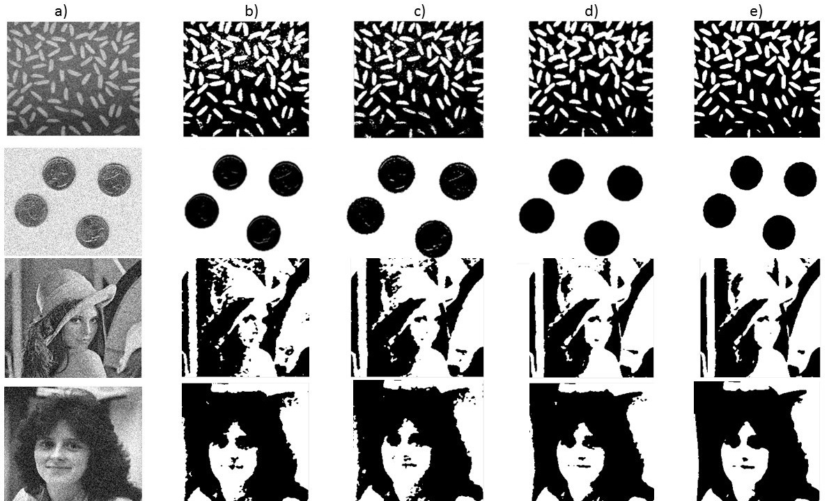
Figure 11: Segmentation results for four samples of natural images (each sample in one row). (a) original image, semented image by (b) ASCI, (c) FCM-AWA, (d) NCM and (e) the proposed method.

For natural images, FCM–AWA is set with parameters: $m=2$, $\alpha=50$, $\varepsilon=10^{-3}$, $r=1$, $k_{0}=0.45$ and $k_{1}=0.65$.

4.6 Medical image dataset

Optical coherence tomography (OCT) is a non-invasive and non-contact imaging method for eye retina which is extensively used clinically for the diagnosis and follow-up of patients with diabetic macular edema (DME) and age-related macular degeneration (AMD). DME and AMD, manifested by fluid regions within the retina and retinal thickening, is caused by fluid leakage from damaged macular blood vessels [43, 67]. In this research, the proposed clustering algorithm is applied to cluster OCT images for fluid segmentation. For this purpose, optima OCT dataset including $196$ images from $4$ patients ($49$ images per subject) is used. It should be noted that fluid segmentation in OCT images needs pre-processing, post-processing and layer segmentation. For these steps, we have used the proposed methods in [43] since these steps are out of the scope of this research. Table 9 and 10 reports average dice coefficients, precision and sensitivity of the proposed method and methods in [42, 43] and [58, 59, 60, 61, 62]. The proposed method achieved the best average sensitivity of $90.59$ and $89.10$ in comparison with manual expert $1$ and manual expert $2$, respectively. For dice coefficient and precision measures, methods in [42] and [58] achieved the best performance. Four samples of OCT images including 1)intra-retinal and sub-retinal fluid, 2)intra-retinal fluid with detached memberance, 3)intera-retinal fluid with hard exudate and hyper-reflective regions and 4) intra-retinal fluid, are segmented by the proposed clustering method in Figs. 12-15, respectively.

Table 9: Dice coefficients, sensitivity and precision of different method in comparison with manual expert 1 segmentation results.

	Sub	GC[58]	KGC[59]	Method in [60]	Method in [61]	Method in [62]	Method in [42]	Method in [43]	Prop. Method
Dice Coeff.	1	73.49	80.43	71.4	61	72	82.96	83.4	81.11
	2	73.9	55.1	45.49	79	84	78.11	59.5	65.8
	3	78.46	75.35	69.54	43	72	82.23	71.3	77.94
	4	78.12	71.78	71.15	46	64	80.75	70.75	66.6
	Ave.	75.99	70.66	64.39	57.25	73	81.01	70.02	72.8
Sensitivity	1	70.81	82.19	72.49	NA	NA	84.43	87.6	88.95
	2	96.79	99.04	70.45	NA	NA	98.94	97.2	97.42
	3	75.72	85.13	47.38	NA	NA	85.18	85.4	85.58
	4	78.78	80.59	77.79	NA	NA	84.49	87.2	90.44
	Ave.	80.52	86.73	67.02	NA	NA	88.26	89.35	90.59
Precision	1	93	85.06	54.87	NA	NA	84.03	84.4	81.02
	2	74.36	54.18	51.12	NA	NA	78.48	59.5	65.52
	3	94.89	79.88	30.93	NA	NA	85.45	77.1	82.07
	4	96.97	88.62	54.98	NA	NA	93.2	71.6	71.1
	Ave.	89.8	76.93	47.97	NA	NA	85.29	73.15	74.92

Table 10: Dice coefficients, sensitivity and precision of different method in comparison with manual expert 2 segmentation results..

	Sub	GC[58]	KGC[59]	Method in [60]	Method in [61]	Method in [62]	Method in [42]	Method in [43]	Prop. Method
Dice Coeff.	1	72.96	79.1	68.17	56	76	82.9	81.86	80.03
	2	71.68	55.11	45.81	76	84	79.09	57.46	63.55
	3	82.33	79.34	65.01	42	75	80.36	79.09	81.09
	4	77.91	71.56	72.55	45	67	80.87	65.59	70.52
	Ave.	76.22	71.27	62.88	54.75	75.5	80.8	71	73.79
Sensitivity	1	69.95	78.56	66.75	NA	NA	80.94	83.03	84.45
	2	92.25	94.54	64.71	NA	NA	94.45	92.56	92.76
	3	81.49	90.95	54.84	NA	NA	90.75	91.57	90
	4	78.54	80.22	77.56	NA	NA	83.7	86.24	89.21
	Ave.	80.55	86.06	65.96	NA	NA	87.46	88.35	89.1
Precision	1	95.71	86.55	59.61	NA	NA	87.53	87.3	83.37
	2	74.45	54.14	51.34	NA	NA	78.58	59.61	65.54
	3	96.1	79.96	37.99	NA	NA	85.48	77.21	82.79
	4	97.24	88.99	59.5	NA	NA	93.58	72.36	71.79
	Ave.	90.87	77.41	52.11	NA	NA	86.29	74.62	75.87

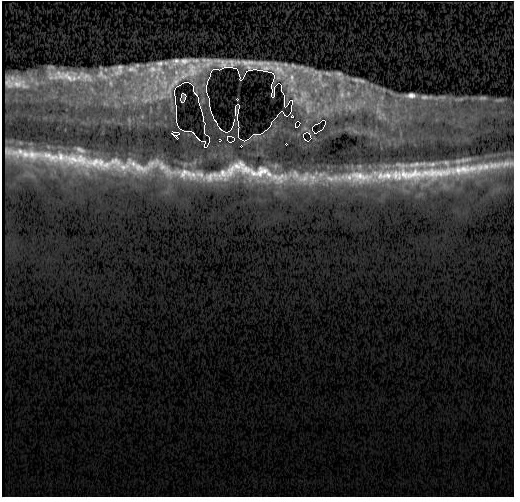
Figure 12: Segmented fluid regions by the proposed clustering method in OCT image with intra-retinal and sub-retinal fluid regions.

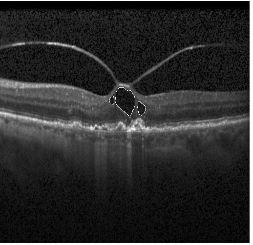
Figure 13: Segmented fluid regions by the proposed clustering method in OCT image with intra-retinal and detached memberance.

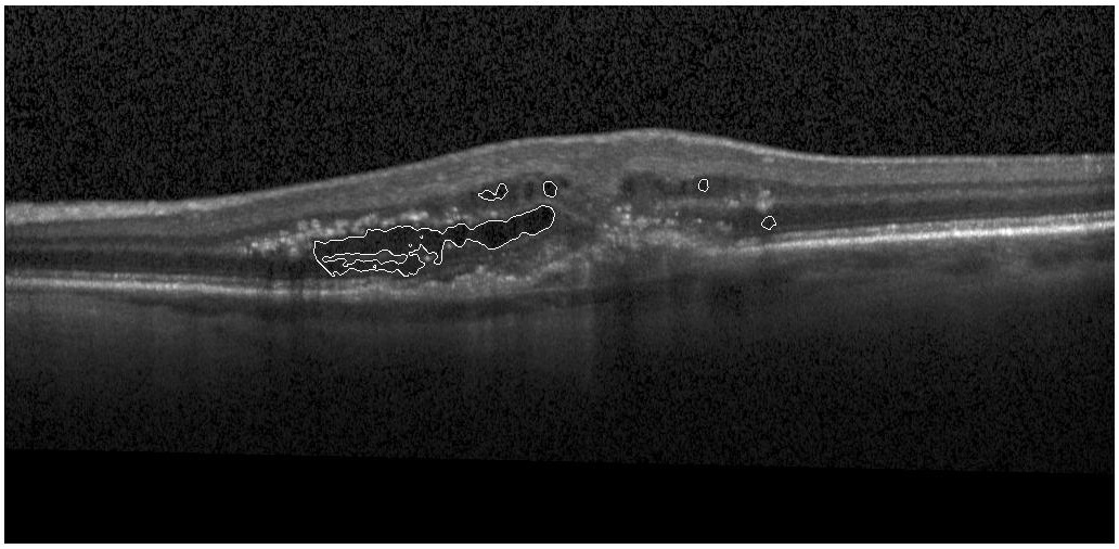
Figure 14: Segmented fluid regions by the proposed clustering method in OCT image with intra-retinal fluid and hard exudate and hyper-reflection regions.

Figure 15: Segmented fluid regions by the proposed clustering method in OCT image with intra-retinal fluid.

5 Discussion

In this section, advantages and disadvantages of the proposed method are discussed. Considering boundary cluster to handle boundary points in methods such as NCM has two side effects which are highly correlated to each other. First, there are points between boundary cluster and a main cluster such as points $5$ and $7$ in $X12$; 5, 7, 11 and $13$ in $X19$; 5, 7, 11, 13, 17 and $19$ in $X24$; 3, 6, 9, 25, 28 and $31$ in $X35$. These points are not assigned to a main cluster with a high certainty. The reason is that such points are located in the same distance from the center of the main cluster and the center of boundary cluster. Second, such points displace center of the main clusters.

Consider cluster $1$ in $X35$. Points $23,5$ and $22$ in $X35$ have the almost same distance from the main cluster center (point $3$) and boundary cluster center (point $6$). Therefore, assigned membership degree of such points to the main cluster and boundary cluster is around $0.50$. Points $21,1$ and $20$ have the higher membership degrees$(T_{i,j})$ to the main cluster in comparison with points $23,5$ and $22$. In NCM, cluster center is in a direct correlation with $T_{i,j}$:

$$c_{j}\approx\sum_{i=1}^{N}(w_{1}T_{i,j})^{m}x_{i}$$ (27)

Therefore, cluster center around point $3$ is forced to move toward points $21$, $1$ and $20$. This condition is same for other clusters in $X35$.

When cluster centers are far away from their correct positions (see Fig. 16(a)), in the next iteration, since points $21,1$ and $20$ are closer to cluster center in comparison with points $23,5$ and $22$, their memberships to the main cluster will be stronger. Therefore, these issues are affected by each other in the next iterations of cost function minimization.

In the proposed method, these issues are addressed by proposing a cost function and ignoring boundary cluster. As it is depicted in Fig. 16, the proposed method is robust and main cluster centers are not forced to be far away from boundary points. Reported results demonstrate how the proposed method handles boundary points and points between boundary points and main cluster centers.

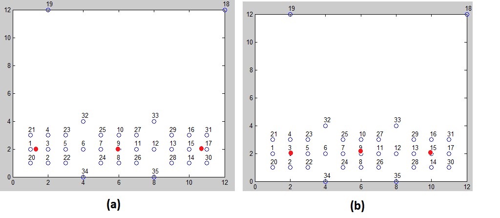
Figure 16: Cluster centers computed by: (a): NCM and (b): the proposed method.

As it is shown in Fig. 17, boundary points have a same distance from main cluster centers. In clustering algorithms, when cluster centers are converged; without significant changes in subsequent iterations; for data point $x_{i}$, term $||x_{i}-c_{j}||$ has the same quantity for all cluster centers $(j={1,2,...,K})$. It leads membership degree $x_{i}$ to cluster center $j$ ($T_{i,j}$) to be almost same for all clusters. We have used this property to distinguish boundary points.

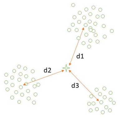
Figure 17: Boundary points.

The main problem in clustering is determining the number of main clusters (K). This issue is domain-specific and should be determined under expert supervision. Here, in each experiment $K$ is determined from a context knowledge. It should be noted that inappropriate $K$ affects clustering results significantly. Also, although benefits of NS theory and some aspects of data clustering such as indeterminacy is considered in the proposed cost function, cost function minimization suffers from local optimum points. Finally, although the proposed indeterminacy definition in neutrosophic domain is appropriate for density-based and center-based clustering, it is not working well on non-density cases such as contiguous-based and nonlinear-shape clusters.

6 Conclusion

In this research, an effective clustering method was proposed in NS domain. For this task, data indeterminacy was proposed based on density properties of data in NS domain to control outlier and boundary points followed by proposing a cost function in NS domain. Two types of clusters including main clusters and noisy cluster are considered in the proposed cost function. Experiments on different datasets including diamond datasets; UCI datasets, artificial and natural images; and medical images showed that the proposed method not only handle outlier and boundary points but also outperforms existing methods in both scatter data clustering and image segmentation. Future efforts will be directed towards introducing indeterminacy in NS domain to supervised methods such as deep convolutional neural networks. Future efforts will be also directed towards proposing methods in neutrosophic domain for handling contiguous-based and nonlinear-shape clusters.

References

References

- [1] R. Xu, D. Wunsch, Survey of clustering algorithms, IEEE Transactions on neural networks 16 (3) (2005) 645–678.
- [2] S. S. Khan, A. Ahmad, Cluster center initialization algorithm for k-modes clustering, Expert Systems with Applications 40 (18) (2013) 7444–7456.
- [3] I. Heloulou, M. S. Radjef, M. T. Kechadi, Automatic multi-objective clustering based on game theory, Expert Systems with Applications 67 (2017) 32–48.
- [4] S. Saha, A. K. Alok, A. Ekbal, Brain image segmentation using semi-supervised clustering, Expert Systems with Applications 52 (2016) 50–63.
- [5] R. Ramon-Gonen, R. Gelbard, Cluster evolution analysis: Identification and detection of similar clusters and migration patterns, Expert Systems with Applications 83 (2017) 363–378.
- [6] A. Baraldi, P. Blonda, A survey of fuzzy clustering algorithms for pattern recognition. i, IEEE Transactions on Systems, Man, and Cybernetics, Part B (Cybernetics) 29 (6) (1999) 778–785.
- [7] Y. Guo, A. Sengur, Ncm: Neutrosophic c-means clustering algorithm, Pattern Recognition 48 (8) (2015) 2710–2724.
- [8] A. R. Webb, Statistical pattern recognition, John Wiley & Sons, 2003.
- [9] K. Wagstaff, C. Cardie, S. Rogers, S. Schrödl, et al., Constrained k-means clustering with background knowledge, in: ICML, Vol. 1, 2001, pp. 577–584.
- [10] D. Arthur, S. Vassilvitskii, k-means++: The advantages of careful seeding, in: Proceedings of the eighteenth annual ACM-SIAM symposium on Discrete algorithms, Society for Industrial and Applied Mathematics, 2007, pp. 1027–1035.
- [11] S. Arora, P. Raghavan, S. Rao, Approximation schemes for euclidean k-medians and related problems, in: Proceedings of the thirtieth annual ACM symposium on Theory of computing, ACM, 1998, pp. 106–113.
- [12] M. Zhang, L. Zhang, H. Cheng, A neutrosophic approach to image segmentation based on watershed method, Signal Processing 90 (5) (2010) 1510–1517.
- [13] J. C. Bezdek, Objective function clustering, in: Pattern recognition with fuzzy objective function algorithms, Springer, 1981, pp. 43–93.
- [14] M. Ménard, C. Demko, P. Loonis, The fuzzy c+ 2-means: solving the ambiguity rejection in clustering, Pattern recognition 33 (7) (2000) 1219–1237.
- [15] M.-S. Yang, K.-L. Wu, J.-N. Hsieh, J. Yu, Alpha-cut implemented fuzzy clustering algorithms and switching regressions, IEEE Transactions on Systems, Man, and Cybernetics, Part B (Cybernetics) 38 (3) (2008) 588–603.
- [16] J. Yu, Q. Cheng, H. Huang, Analysis of the weighting exponent in the fcm, IEEE Transactions on Systems, Man, and Cybernetics, Part B (Cybernetics) 34 (1) (2004) 634–639.
- [17] D. E. Gustafson, W. C. Kessel, Fuzzy clustering with a fuzzy covariance matrix, in: Decision and Control including the 17th Symposium on Adaptive Processes, 1978 IEEE Conference on, IEEE, 1979, pp. 761–766.
- [18] R. Krishnapuram, J. M. Keller, A possibilistic approach to clustering, IEEE transactions on fuzzy systems 1 (2) (1993) 98–110.
- [19] N. R. Pal, K. Pal, J. C. Bezdek, A mixed c-means clustering model, in: Fuzzy Systems, 1997., Proceedings of the Sixth IEEE International Conference on, Vol. 1, IEEE, 1997, pp. 11–21.
- [20] M. Roubens, Pattern classification problems and fuzzy sets, Fuzzy sets and systems 1 (4) (1978) 239–253.
- [21] R. J. Hathaway, J. W. Davenport, J. C. Bezdek, Relational duals of the c-means clustering algorithms, Pattern recognition 22 (2) (1989) 205–212.
- [22] S. Sen, R. Dave, Clustering of relational data containing noise and outliers, in: Fuzzy Systems Proceedings, 1998. IEEE World Congress on Computational Intelligence., The 1998 IEEE International Conference on, Vol. 2, IEEE, 1998, pp. 1411–1416.
- [23] M.-H. Masson, T. Denoeux, Ecm: An evidential version of the fuzzy c-means algorithm, Pattern Recognition 41 (4) (2008) 1384–1397.
- [24] M.-H. Masson, T. Denœux, Recm: Relational evidential c-means algorithm, Pattern Recognition Letters 30 (11) (2009) 1015–1026.
- [25] X. Li, Q. Han, B. Qiu, A clustering algorithm using skewness-based boundary detection, Neurocomputing 275 (2018) 618–626.
- [26] G. Cui, X. Li, Y. Dong, Subspace clustering guided convex nonnegative matrix factorization, Neurocomputing 292 (2018) 38–48.
- [27] Q. Tong, X. Li, B. Yuan, Efficient distributed clustering using boundary information, Neurocomputing 275 (2018) 2355–2366.
- [28] F. Hammou, K. Hammouche, J.-G. Postaire, Convexity dependent anisotropic diffusion for mode detection in cluster analysis, Neurocomputing.
- [29] A. Saxena, M. Prasad, A. Gupta, N. Bharill, O. P. Patel, A. Tiwari, M. J. Er, W. Ding, C.-T. Lin, A review of clustering techniques and developments, Neurocomputing 267 (2017) 664–681.
- [30] F. Smarandache, Neutrosophic logic and set.
- [31] F. Smarandache, A Unifying Field in Logics: Neutrosophic Logic. Neutrosophy, Neutrosophic Set, Neutrosophic Probability: Neutrosophic Logic: Neutrosophy, Neutrosophic Set, Neutrosophic Probability, Infinite Study, 2003.
- [32] Y. Guo, H.-D. Cheng, New neutrosophic approach to image segmentation, Pattern Recognition 42 (5) (2009) 587–595.
- [33] M. Zhang, L. Zhang, H. Cheng, A neutrosophic approach to image segmentation based on watershed method, Signal Processing 90 (5) (2010) 1510–1517.
- [34] A. Sengur, Y. Guo, Color texture image segmentation based on neutrosophic set and wavelet transformation, Computer Vision and Image Understanding 115 (8) (2011) 1134–1144.
- [35] A. Heshmati, M. Gholami, A. Rashno, Scheme for unsupervised colour–texture image segmentation using neutrosophic set and non-subsampled contourlet transform, IET Image Processing 10 (6) (2016) 464–473.
- [36] Y. Guo, Y. Akbulut, A. Şengür, R. Xia, F. Smarandache, An efficient image segmentation algorithm using neutrosophic graph cut, Symmetry 9 (9) (2017) 185.
- [37] B. Salafian, R. Kafieh, A. Rashno, M. Pourazizi, S. Sadri, Automatic segmentation of choroid layer in edi oct images using graph theory in neutrosophic space, arXiv preprint arXiv:1812.01989.
- [38] Y. Guo, A. Şengür, J. Ye, A novel image thresholding algorithm based on neutrosophic similarity score, Measurement 58 (2014) 175–186.
- [39] Y. Guo, A. Şengür, A novel image edge detection algorithm based on neutrosophic set, Computers & Electrical Engineering 40 (8) (2014) 3–25.
- [40] A. Rashno, F. Smarandache, S. Sadri, Refined neutrosophic sets in content-based image retrieval application, in: Machine Vision and Image Processing (MVIP), 2017 10th Iranian Conference on, IEEE, 2017, pp. 197–202.
- [41] A. Rashno, S. Sadri, Content-based image retrieval with color and texture features in neutrosophic domain, in: Pattern Recognition and Image Analysis (IPRIA), 2017 3rd International Conference on, IEEE, 2017, pp. 50–55.
- [42] A. Rashno, B. Nazari, D. D. Koozekanani, P. M. Drayna, S. Sadri, H. Rabbani, K. K. Parhi, Fully-automated segmentation of fluid regions in exudative age-related macular degeneration subjects: Kernel graph cut in neutrosophic domain, PloS one 12 (10) (2017) e0186949.
- [43] A. Rashno, D. D. Koozekanani, P. M. Drayna, B. Nazari, S. Sadri, H. Rabbani, K. K. Parhi, Fully-automated segmentation of fluid/cyst regions in optical coherence tomography images with diabetic macular edema using neutrosophic sets and graph algorithms, IEEE Transactions on Biomedical Engineering.
- [44] A. Rashno, K. K. Parhi, B. Nazari, S. Sadri, H. Rabbani, P. Drayna, D. D. Koozekanani, Automated intra-retinal, sub-retinal and sub-rpe cyst regions segmentation in age-related macular degeneration (amd) subjects, Investigative Ophthalmology & Visual Science 58 (8) (2017) 397–397.
- [45] K. K. Parhi, A. Rashno, B. Nazari, S. Sadri, H. Rabbani, P. Drayna, D. D. Koozekanani, Automated fluid/cyst segmentation: A quantitative assessment of diabetic macular edema, Investigative Ophthalmology & Visual Science 58 (8) (2017) 4633–4633.
- [46] J. Kohler, A. Rashno, K. K. Parhi, P. Drayna, S. Radwan, D. D. Koozekanani, Correlation between initial vision and vision improvement with automatically calculated retinal cyst volume in treated dme after resolution, Investigative Ophthalmology & Visual Science 58 (8) (2017) 953–953.
- [47] Y. Guo, A. S. Ashour, B. Sun, A novel glomerular basement membrane segmentation using neutrsophic set and shearlet transform on microscopic images, Health information science and systems 5 (1) (2017) 15.
- [48] Y. Guo, Ü. Budak, A. Şengür, F. Smarandache, A retinal vessel detection approach based on shearlet transform and indeterminacy filtering on fundus images, Symmetry 9 (10) (2017) 235.
- [49] S. K. Siri, M. V. Latte, Combined endeavor of neutrosophic set and chan-vese model to extract accurate liver image from ct scan, Computer methods and programs in biomedicine 151 (2017) 101–109.
- [50] S. K. Siri, M. V. Latte, A novel approach to extract exact liver image boundary from abdominal ct scan using neutrosophic set and fast marching method, Journal of Intelligent Systems.
- [51] M. Lotfollahi, M. Gity, J. Y. Ye, A. M. Far, Segmentation of breast ultrasound images based on active contours using neutrosophic theory, Journal of Medical Ultrasonics (2017) 1–8.
- [52] Y. Akbulut, A. Sengur, Y. Guo, F. Smarandache, Ns-k-nn: Neutrosophic set-based k-nearest neighbors classifier, Symmetry 9 (9) (2017) 179.
- [53] S. Dhar, M. K. Kundu, Accurate segmentation of complex document image using digital shearlet transform with neutrosophic set as uncertainty handling tool, Applied Soft Computing 61 (2017) 412–426.
- [54] Y. Akbulut, A. Şengür, Y. Guo, K. Polat, Kncm: Kernel neutrosophic c-means clustering, Applied Soft Computing 52 (2017) 714–724.
- [55] J. C. Bezdek, R. Ehrlich, W. Full, Fcm: The fuzzy c-means clustering algorithm, Computers & Geosciences 10 (2-3) (1984) 191–203.
- [56] S. K. Pal, Fuzzy tools for the management of uncertainty in pattern recognition, image analysis, vision and expert systems, International journal of systems science 22 (3) (1991) 511–549.
- [57] J. Kang, L. Min, Q. Luan, X. Li, J. Liu, Novel modified fuzzy c-means algorithm with applications, Digital signal processing 19 (2) (2009) 309–319.
- [58] Y. Boykov, G. Funka-Lea, Graph cuts and efficient nd image segmentation, International journal of computer vision 70 (2) (2006) 109–131.
- [59] M. B. Salah, A. Mitiche, I. B. Ayed, Multiregion image segmentation by parametric kernel graph cuts, IEEE Transactions on Image Processing 20 (2) (2011) 545–557.
- [60] M. Esmaeili, A. M. Dehnavi, H. Rabbani, F. Hajizadeh, Three-dimensional segmentation of retinal cysts from spectral-domain optical coherence tomography images by the use of three-dimensional curvelet based k-svd, Journal of medical signals and sensors 6 (3) (2016) 166.
- [61] L. de Sisternes, J. Hong, T. Leng, D. L. Rubin, A machine learning aproach for device-independent automated segmentation of retinal cysts in spectral domain optical cohorence tomography images.
- [62] F. G. Venhuizena, M. Grinsvena, C. B. Hoyngb, T. Theelenb, B. Ginnekena, C. I. Sancheza, Vendor independent cyst segmentation in retinal sd-oct volumes using a combination of multiple scale convolutional neural networks, Medical Image Computing and Computer Assisted Intervention-Challenge on Retinal Cyst Segmentation.
- [63] M. Ménard, C. Demko, P. Loonis, The fuzzy c+ 2-means: solving the ambiguity rejection in clustering, Pattern recognition 33 (7) (2000) 1219–1237.
- [64] M. Roubens, Pattern classification problems and fuzzy sets, Fuzzy sets and systems 1 (4) (1978) 239–253.
- [65] N. R. Pal, K. Pal, J. M. Keller, J. C. Bezdek, A possibilistic fuzzy c-means clustering algorithm, IEEE transactions on fuzzy systems 13 (4) (2005) 517–530.
- [66] N.-E. El Harchaoui, M. A. Kerroum, A. Hammouch, M. Ouadou, D. Aboutajdine, Unsupervised approach data analysis based on fuzzy possibilistic clustering: application to medical image mri, Computational intelligence and neuroscience 2013 (2013) 10.
- [67] A. Rashno, D. D. Koozekanani, K. K. Parhi, Oct fluid segmentation using graph shortest path and convolutional neural network, in: 2018 40th Annual International Conference of the IEEE Engineering in Medicine and Biology Society (EMBC), IEEE, 2018, pp. 3426–3429.