Hybrid Wasserstein Distance and Fast Distribution Clustering
Isabella Verdinelli and Larry Wasserman
Department of Statistics and Data Science
Carnegie Mellon University
December 27 2018

We define a modified Wasserstein distance for distribution clustering which inherits many of the properties of the Wasserstein distance but which can be estimated easily and computed quickly. The modified distance is the sum of two terms. The first term — which has a closed form — measures the location-scale differences between the distributions. The second term is an approximation that measures the remaining distance after accounting for location-scale differences. We consider several forms of approximation with our main emphasis being a tangent space approximation that can be estimated using nonparametric regression. We evaluate the strengths and weaknesses of this approach on simulated and real examples.

1 Introduction

The Wassertstein distance has attracted much attention lately because it has many appealing properties. (Panaretos and Zemel (2018); Sommerfeld and Munk (2018)). It is especially useful as a tool for clustering a set of distributions $P_{1},\ldots,P_{N}$ because it captures key shape characteristics of the distributions. But the Wasserstein distance is difficult to compute and difficult to estimate from samples. In this paper we introduce a modified Wasserstein distance that can be estimated and computed quickly.

Wasserstein Distance. If $X\in\mathbb{R}^{d}$ is a random vector with distribution $P$ and $Y\in\mathbb{R}^{d}$ is a random vector with distribution $Q$ then, for $p\geq 1$, the $p$-Wasserstein distance is defined by

$$W_{p}(P,Q)\equiv W_{p}(X,Y)=\left(\inf_{J}\int||x-y||^{p}\,dJ(x,y)\right)^{1/p}$$ (1)

where the infimum is over all joint distributions $J$ for $(X,Y)$ such that $X$ has marginal $P$ and $Y$ has marginal $Q$. The minimizer $J^{*}$ is called the optimal transport plan or the optimal coupling. Figure 1 illustrates an example of a coupling $J$. In this paper we will focus on the case $p=2$ and then we write $W(P,Q)$ or $W(X,Y)$ instead of $W_{2}(P,Q)$ or $W_{2}(X,Y)$.

The modified distance that we propose is

$$H^{2}(X,Y)=W^{2}(Z_{X},Z_{Y})+W_{\dagger}^{2}(\widetilde{X},\widetilde{Y})$$ (2)

where

$$Z_{X}\sim N(\mu_{X},\Sigma_{X}),\ \ \ \ \ \ \widetilde{X}=\Sigma^{-1/2}_{X}(X-\mu_{X})$$

$$Z_{Y}\sim N(\mu_{Y},\Sigma_{Y}),\ \ \ \ \ \ \widetilde{Y}=\Sigma^{-1/2}_{Y}(Y-\mu_{Y}),$$

$\mu_{X}=\mathbb{E}[X]$, $\mu_{Y}=\mathbb{E}[Y]$, $\Sigma_{X}={\rm Var}[X]$ and $\Sigma_{Y}={\rm Var}[Y]$ and $W_{\dagger}$ is a distance between the centered and scaled variables $\widetilde{X}$ and $\widetilde{Y}$. We consider several possible choices for $W_{\dagger}$. We mainly focus on the case where $W_{\dagger}(\widetilde{X},\widetilde{Y})$ is a tangent space approximation to $W(\widetilde{X},\widetilde{Y})$ as defined by Wang et al. (2013). The details of this tangent approximation are given in Section 3. Our version of the tangent space distance is a bit different than the original implementation as we use a combination of density estimation, permutation smoothing and subsampling. We will call $H$ the hybrid distance. We will consider other choices for $W_{\dagger}(\widetilde{X},\widetilde{Y})$ in Section 6.

The first term in (2) measures location-scale differences between the two distributions, is available in closed form (see equation 4) and can be estimated at a $n^{-1/2}$ rate where $n$ is the sample size. The second term captures any remaining non-linear differences.

Figure 1: This is an illustration of a coupling $J$ with given marginals for $X$ and $Y$. Generally, there are many such joint distributions.

Distribution Clustering. As mentioned above, our main motivation is “distribution clustering” which requires repeatedly computing distances. Suppose, for example, that we want to cluster a set of distributions $P_{1},\ldots,P_{N}$. Typically, these are empirical distributions corresponding to datasets ${\cal D}_{1},\ldots,{\cal D}_{N}$. Given a metric $d$ on the set of probability distributions, we can adapt existing methods — such as hierarchical clustering and $k$-means clustering — to the problem of clustering distributions. But if we use Wasserstein distance then the calculations become onerous since we need to compute many distances. For example, suppose we want to perform agglomerative hierarchical clustering. First we need to compute the $N(N-1)/2$ distances $W_{p}(P_{i},P_{j})$. If we decide to cluster, say $P_{1}$ and $P_{2}$, we need to combine the corresponding datasets ${\cal D}_{1}$ and ${\cal D}_{2}$. Then we need to compute the distance between the new empirical measure corresponding to ${\cal D}_{1}\bigcup{\cal D}_{2}$ and all the other distributions. Each stage of the hierarchical clustering involves recalculating the distances. Similarly, if we use $k$-means clustering we need to iterate between assigning points to clusters and computing centroids. Computing the centroid — also known as a barycenter — with respect to the Wasserstein distance is computationally expensive. We show that replacing $W$ with $H$ significantly reduces the computational burden without sacrificing accurate clustering.

Related Work. Our works builds on Wang et al. (2013) who introduced the idea of using a tangent space approximation to Wasserstein distance. Their motivation was image processing and their implementation of the idea is quite different than our version. We also make use of subsampling approximations which were suggested in Sommerfeld et al. (2018). The Gaussian approximation $W(Z_{X},Z_{Y})$ is an example of a linear approximation. Optimal linear approximations to Wasserstein distance are studied in Kuang and Tabak (2017). An important reference on clustering distributions with Wasserstein distance is del Barrio et al. (2017) which not only introduces the idea of distribution clustering in this way, but also proposes a trimming procedure to create robust clusterings. We do not consider robustness in this paper but we note that combining ideas from del Barrio et al. (2017) with the ideas in this paper is an interesting future direction. Wasserstein clustering is also studied in Ho et al. (2017) in the context of hierarchical models. That paper not only clusters distributions but, simultaneously, clusters data within each distribution.

Paper Outline. In Section 2 we review the Wasserstein distance. In Section 3 we give the details of the proposed modified distance. In Section 4 we define several versions of k-means distribution clustering. Section 5 gives some examples. In Section 6 we briefly explain how our ideas can be used for hierarchical clustering and mean-shift clustering. In Section 7 we discuss some different versions of hybridization. Section 8 contains a discussion and concluding remarks.

2 Wasserstein Distance

In this section we give a brief review of the Wasserstein distance and we explain why it is useful for distribution clustering. An excellent reference on Wasserstein distance is Villani (2003). Recall that the Wasserstein distance is defined in equation (1).

Explicit Expressions. In general, there is no closed form expression for $W_{p}$. There are three notable exceptions.

(i) When $d=1$, the distance can be written explicitly as

$$W_{p}(P,Q)=\left(\int_{0}^{1}|F^{-1}(z)-G^{-1}(z)|^{p}\right)^{1/p}$$

where $F(x)=P(X\leq x)$ and $G(y)=Q(Y\leq y)$.

(ii) If $P_{n}$ is the empirical distribution of a dataset $X_{1},\ldots,X_{n}$ and $Q_{n}$ is the empirical distribution of another dataset $Y_{1},\ldots,Y_{n}$ of the same size, then the distance takes the form

$$W_{p}^{p}(P_{n},Q_{n})=\min_{\pi}\frac{1}{n}\sum_{i=1}^{n}||X_{i}-Y_{\pi(i)}||^{p}$$

where the minimum is over all permutations. This minimization can be done using various algorithms such as the Hungarian algorithm (Kuhn (1955)) which takes time $O(n^{3})$. When $d=1$ this further simplifies to

$$W_{p}(P_{n},Q_{n})=\left(\frac{1}{n}\sum_{i=1}^{n}|X_{(i)}-Y_{(i)}|^{p}\right)^{1/p}$$ (3)

where $X_{(1)}\leq\cdots\leq X_{(n)}$ and $Y_{(1)}\leq\cdots\leq Y_{(n)}$ are the order statistics.

(iii) The distance has a simple expression is the Gaussian case (or more generally, for location-scale families). Suppose that $X\sim N(\mu_{X},\Sigma_{X})$ and $Y\sim N(\mu_{Y},\Sigma_{Y})$. Then

$$W^{2}(P,Q)\equiv W^{2}(X,Y)=||\mu_{X}-\mu_{Y}||^{2}+{\rm B}^{2}(\Sigma_{X},\Sigma_{Y})$$ (4)

where

$${\rm B}^{2}(\Sigma_{X},\Sigma_{Y})={\rm tr}(\Sigma_{1})+{\rm tr}(\Sigma_{2})-2{\rm tr}\Bigl{[}\Bigl{(}\Sigma_{X}^{1/2}\Sigma_{Y}\Sigma_{X}^{1/2}\Bigr{)}^{1/2}\Bigr{]}$$ (5)

is the Bures distance (Bhatia et al. (2018)) between $\Sigma_{X}$ and $\Sigma_{Y}$. See Givens et al. (1984) and Rippl et al. (2016). From now on, we refer to (4) as the Gaussian Wasserstein distance and we denote this as $G^{2}(X,Y)=||\mu_{X}-\mu_{Y}||^{2}+{\rm B}^{2}(\Sigma_{X},\Sigma_{Y})$.

The Monge Distance and Transport Maps. A related distance is the Monge distance defined by

$$\left(\inf_{T}\int||x-T(x)||^{p}dP(x)\right)^{1/p}$$ (6)

where the infimum is over all maps $T$ such that $T(X)\sim Q$. When a minimizer exists, this corresponds to the Wasserstein distance and the map $T$ is called the optimal transport map. In this case the optimal coupling $J^{*}$ is a degenerate distribution on the set $\{(x,T(x))\}$. But, the minimizer might not exist. Consider $P=\delta_{0}$ and $Q=(1/2)\delta_{-1}+(1/2)\delta_{1}$ where $\delta_{a}$ denotes a point mass at $a$. In this case, there is no map $T$ such that $T(X)\sim Q$. In contrast, an optimal coupling always exists and can be thought of as defining a transport plan that allows the mass to be split and assigned to many locations. A sufficient condition for the existence of a unique optimal transport map is that both $P$ and $Q$ be absolutely continuous with respect to Lebesgue measure. In the Gaussian case, the optimal transport map is the linear map

$$L(x)=\mu_{Y}+\Sigma_{Y}^{1/2}\Sigma_{X}^{-1/2}(x-\mu_{X}).$$

Barycenters. Given a set of distributions $P_{1},\ldots,P_{N}$, the barycenter, with respect to non-negative weights $\lambda_{1},\ldots,\lambda_{N}$, is defined to be the distribution $P$ that minimizes $\sum_{j}\lambda_{j}W^{2}(P,P_{j})$. (In this paper, we will always use $\lambda_{j}=1/N$.) There is a substantial literature on finding methods to compute the barycenter. In the special case that each $P_{j}$ is Gaussian, the barycenter takes a special form. Let $P_{j}=N(\mu_{j},\Sigma_{j})$ for $j=1,\ldots,N$. Then the barycenter $P$ is $N(\mu,\Sigma)$ where $\mu=N^{-1}\sum_{j}\lambda_{j}\mu_{j}$ and $\Sigma$ is the unique, symmetric, positive definite matrix satisfying the fixed point equation

$$\Sigma=\sum_{j}\lambda_{j}(\Sigma^{1/2}\Sigma_{j}\Sigma^{1/2})^{1/2}.$$ (7)

The same holds for any location-scale family; see Álvarez-Esteban et al. (2016). In one dimension, the barycenter of $P_{1},\ldots,P_{N}$ is the distribution $P$ with cdf $F$ where $F^{-1}(u)=\sum_{j}\lambda_{j}F_{j}^{-1}(u)$.

Key Properties. There has been a surge of interest in the Wasserstein distance in statistics and machine learning lately. This is because the distance has a number of useful properties. Here we review three key properties, namely: (1) sensitivity to underlying geometry, (2) comparability of discrete and continuous distributions and (3) shape preservation.

1. The Wasserstein distance is sensitive to the underlying geometry. Consider the distributions $P_{1}=\delta_{0},P_{2}=\delta_{\epsilon}$ and $P_{3}=\delta_{100}$ where $\delta_{a}$ denotes a point mass at $a$ and $\epsilon>0$ is a small positive number. Then $W(P_{1},P_{2})\approx 0$, $W(P_{1},P_{3})\approx W(P_{2},P_{3})\approx 100$. On the other hand, consider the total variation distance $d_{\rm TV}$. Then $d_{\rm TV}(P_{1},P_{2})=d_{\rm TV}(P_{1},P_{3})=d_{\rm TV}(P_{2},P_{3})=1$. So the total variation distance fails to capture our intuition that $P_{1}$ and $P_{2}$ are close while $P_{3}$ is far. The same is true for Hellinger distance and Kullback-Leibler distance.

2. The Wasserstein distance permits direct comparison between discrete and continuous distribution. If $P_{1}$ is continous and $P_{2}$ is discrete, then, for example, $d_{\rm TV}(P_{1},P_{2})=1$. But $W_{p}(P_{1},P_{2})$ gives reasonable values. For example, suppose that $P_{1}$ is uniform on $[0,1]$ and $P_{2}$ is uniform on $\{1/N,2/N,\ldots,1\}$. Then $d_{\rm TV}(P_{1},P_{2})=1$ for all $N$ but $W_{p}(P_{1},P_{2})=1/N$ which again seems quite intuitive.

3. Shape Preservation. Suppose we have a set of distributions $P_{1},\ldots,P_{N}$. Recall that the barycenter $P$ minimizes $\sum_{j}\lambda_{j}W_{2}^{2}(P,P_{j})$. The barycenter $P$ preserves the shape of the distributions. Specifically, if each $P_{j}$ can be written as a location-scale shift of some distribution $P_{0}$, the $P$ is also a location-scale shift of $P_{0}$. For example, suppose that $P_{1}=N(\mu_{1},\Sigma)$ and that $P_{2}=N(\mu_{2},\Sigma)$. Then the barycenter is $P=N((\mu_{1}+\mu_{2})/2,\Sigma)$. In contrast, the Euclidean average $(1/2)P_{1}+(1/2)P_{2}$ looks nothing like any of the $P_{j}$’s. Figure 2 shows a comparison of the Wasserstein barycenter and the Euclidean average.

Figure 2: Top row: Six Gaussian distributions. Bottom left: The Euclidean average of the six distributions. Bottom right: The Wasserstein barycenter.

3 The Hybrid Distance

Let $X\sim P$ and $Y\sim Q$. Define $Z_{X}\sim N(\mu_{X},\Sigma_{X})$, $Z_{Y}\sim N(\mu_{Y},\Sigma_{Y})$, $\widetilde{X}=\Sigma^{-1/2}_{X}(X-\mu_{X})$, and $\widetilde{Y}=\Sigma^{-1/2}_{Y}(Y-\mu_{Y})$. Our modified distance — which we call the hybrid distance — is

$$H^{2}(X,Y)=W^{2}(Z_{X},Z_{Y})+W_{\dagger}^{2}(\widetilde{X},\widetilde{Y})=G^{2}(X,Y)+W_{\dagger}^{2}(\widetilde{X},\widetilde{Y})$$ (8)

where $W_{\dagger}$ is described below. The first term $W^{2}(Z_{X},Z_{Y})\equiv G^{2}(X,Y)$ has a simple closed form, namely, $||\mu_{X}-\mu_{Y}||^{2}+{\rm B}^{2}(\Sigma_{X},\Sigma_{Y})$ where ${\rm B}(\cdot,\cdot)$ is the Bures distance. Given samples $X_{1},\ldots,X_{n}\sim P$ and $Y_{1},\ldots,Y_{m}\sim Q$, we can estimate $W^{2}(Z_{X},Z_{Y})$ by plugging in sample moments. We then have that $\widehat{W}(Z_{X},Z_{Y})=W(Z_{X},Z_{Y})+O_{P}((n\wedge m)^{-1/2})$; see Rippl et al. (2016). We measure the remaining difference by computing the distance between the standardized variables $\widetilde{X}=\Sigma^{-1/2}_{X}(X-\mu_{X})$, $\widetilde{Y}=\Sigma^{-1/2}_{Y}(Y-\mu_{Y})$ by adapting the method from Wang et al. (2013) which we now describe.

Consider a set of distributions $P_{1},\ldots,P_{N}$. Let $\mu_{j}=\mathbb{E}[X_{j}]$ and $\Sigma_{j}={\rm Var}[X_{j}]$ where $X_{j}\sim P_{j}$. Let $Z_{j}\sim N(\mu_{j},\Sigma_{j})$ and $\widetilde{X}_{j}=\Sigma_{j}^{-1/2}(X_{j}-\mu_{j})$. Let $R$ be a reference measure with density $r$, ($R$ is defined below.) Define

$$W_{\dagger}^{2}(\widetilde{P}_{j},\widetilde{P}_{k})=\int(\psi_{j}(z)-\psi_{k}(z))^{2}dz$$ (9)

where $\psi_{j}(z)=(T_{j}(z)-z)\sqrt{r(z)}$, and $T_{j}$ is the optimal transport map from $\widetilde{P}_{j}$ to $R$. Wang et al. (2013) justify this expression as follows. The set of probability measures endowed with the Wasserstein metric is a Riemannian manifold. Then $\int(\psi_{j}(z)-\psi_{k}(z))^{2}dz$ is the distance between the projections of $\widetilde{P}_{j}$ and $\widetilde{P}_{k}$ onto the tangent space at $R$; Now

$$\int(\psi_{j}(z)-\psi_{k}(z))^{2}dz=\int(T_{j}(z)-T_{k}(z))^{2}dR(z).$$

Hence, if $U_{1},\ldots,U_{m}\sim R$ then

$$\int(\psi_{j}(z)-\psi_{k}(z))^{2}dz=\frac{1}{m}\sum_{s=1}^{m}(T_{j}(U_{s})-T_{k}(U_{s}))^{2}+O_{P}(m^{-1/2}).$$

Figure 3: The space of probability measures equipped with Wasserstein distance is a manifold. The tangent distance between $P$ and $Q$ is the Euclidean distance between the projection of $P$ and $Q$ into the local tangent space at the reference measure $R$.

The hybrid distance is

$$H^{2}(X_{j},X_{k}) =W^{2}(Z_{j},Z_{k})+W_{\dagger}^{2}(\widetilde{X}_{j},\widetilde{X}_{k})$$

$$=||\mu_{j}-\mu_{k}||^{2}+{\rm B}^{2}(\Sigma_{j},\Sigma_{k})+\int(\psi_{j}(z)-\psi_{k}(z))^{2}dz$$

$$=||\mu_{j}-\mu_{k}||^{2}+{\rm B}^{2}(\Sigma_{j},\Sigma_{k})+\int(T_{j}(z)-T_{k}(z))^{2}dR(z)$$

$$\approx\underbrace{||\mu_{j}-\mu_{k}||^{2}}_{\rm location}+\underbrace{{\rm B}^{2}(\Sigma_{j},\Sigma_{k})}_{\rm scale}+\underbrace{\frac{1}{m}\sum_{i}(T_{j}(U_{i})-T_{k}(U_{i}))^{2}}_{\rm shape}$$ (10)

where $U_{1},\ldots,U_{m}\sim R$.

To estimate the distance we need to choose $R$ and estimate $T_{j}$. Wang et al. (2013), motivated by applications in image processing, suggest using $R=N^{-1}\sum_{j}P_{j}$. We take a slightly different approach. Recall that we have datasets ${\cal D}_{1},\ldots,{\cal D}_{N}$ where ${\cal D}_{j}=\{X_{j1},\ldots,X_{jn_{j}}\}$ consists of $n_{j}$ observations with empirical distribution $P_{j}$. Let $\widetilde{D}_{j}=(\widetilde{X}_{js}:\ 1\leq s\leq n_{j})$ denote the normalized observations where $\widetilde{X}_{js}=\widehat{\Sigma}_{j}^{-1/2}(X_{js}-\widehat{\mu}_{j})$. The combined dataset $\widetilde{\cal D}=\bigcup_{j=1}^{N}\widetilde{\cal D}_{j}$ can be regarded as a sample from $\sum_{j}\pi_{j}\widetilde{P_{j}}$ where $\pi_{j}=n_{j}/\sum_{j}n_{j}$ and $\widetilde{P}_{j}$ is the distribution of $\widetilde{X}_{j}$. Let $R$ be the distribution with density $r$ where $r$ is a kernel density estimate obtained from $\widetilde{\cal D}$ using a simple bandwidth rule such as Silverman’s rule (Silverman, 2018). Thus, $R=R_{n}\star K_{h}$ (the convolution) where $R_{n}=\sum_{j}\pi_{j}\widetilde{P}_{j}$ and $K_{h}$ is a kernel with bandwidth $h$. This choice of reference measure is simple and smooth.

Next we have to estimate $T_{j}$. Here we use a variation of nonparametric regression that we call permutation smoothing. The steps are given in Figure 4. The idea is to sample $m$ observations from each dataset and the reference measure $R$. The optimal permutation for matching the samples can be found in $O(m^{3})$ time. This defines a map $T_{j}$ from $m$ points drawn from $\widetilde{P}_{j}$ to $m$ points drawn from $R$. We then extend $T_{j}$ over the whole space by using $r$-nearest neighbor regression. We show in the appendix that it suffices to take $r=1$ to get a consistent estimator of the transport function. This amounts to taking $T_{j}$ to be the piecewise constant over the Voronoi tesselation $V_{1},\ldots,V_{m}$ defined by the point drawn from $\widetilde{P}_{j}$. We can summarize the steps as follows:

$${\rm Gaussian\ approximation}\longrightarrow{\rm subsample}\longrightarrow{\rm permutation\ smoothing}\longrightarrow\ {\rm tangent\ approximation}.$$

Wang et al. (2013) point out that the tangent space approximation is a well-defined distance and need not be thought of as an approximation to the Wasserstein distance. They show that, even when it does not approximate the Wasserstein distance, it still contains valuable information for comparing distributions.

1. Fix an integer $m$. 2. Draw a sample $U_{1},\ldots,U_{m}\sim R$ and draw a subsample $\widetilde{X}_{j1},\ldots,\widetilde{X}_{jm}$ from $\widetilde{\cal D}_{j}$. 3. Find the permutation $\pi_{j}$ that minimizes $\sum_{i=1}^{m}||\widetilde{X}_{ji}-U_{\pi(i)}||^{2}$. This can be done using the Hungarian algorithm and takes $O(m^{3})$ time. 4. Let $V_{j1},\ldots,V_{jm}$ be the Voronoi tesselation defined by $\widetilde{X}_{j1},\ldots,\widetilde{X}_{jm}$. Define $\widehat{T}_{j}(x)=\sum_{s}U_{\pi_{j}(s)}I(x\in V_{s})$ for all $x\in\{U_{1},\ldots,U_{m}\}$.

Figure 4: Permutation smoothing algorithm to estimate transport map.

In the appendix we show that this method is consistent if $n_{j}\to\infty$ and $m\to\infty$. The idea of using subsamples to approximate Wasserstein distance (rather than using subsamples to estimate the transport map to a reference measure as we are doing) was examined carefully in Sommerfeld et al. (2018). For distribution clustering, the subsample size $m$ need not be large. (In our examples we use $m=100$ but we get similar results even using $m=20$). This keeps the computation very fast. Also, note that we only ever evaluate $\widehat{T}_{j}$ on the points $U_{1},\ldots,U_{m}\sim R$.

Remark. Sommerfeld et al. (2018) suggest estimating Wasserstein distance by averaging over subsamples. Similarly, we could repeat our procedure over several subsamples and average the $\widehat{T}_{j}$’s. However, we have not found this to be necessary for distribution clustering.

Remark. We use $r$-nearest neighbor regression with $r=1$. Of course, $r$ can be replaced with a larger value if we want $\widehat{T}_{j}$ to be smooth. However, $r=1$ suffices for consistency.

Finally, we estimate $H^{2}$ by

$$\widehat{H}^{2}(P_{j},P_{k})=||\widehat{\mu}_{j}-\widehat{\mu}_{k}||^{2}+{\rm B}^{2}(\widehat{\Sigma}_{j},\widehat{\Sigma}_{k})+\frac{1}{m}\sum_{s=1}^{m}(\widehat{T}_{j}(U_{s})-\widehat{T}_{k}(U_{s}))^{2}.$$ (11)

The modified distance retains many properties of Wasserstein distance. The following proposition summarizes these facts. The proof is straightforward and is omitted.

Proposition 1

The distance $H$ has the following properties.

1. $H$ is a metric on the space of distributions with densities and finite second moments. In particular, $H(P,Q)=0$ if and only if $P=Q$.

2. $H$ is exact for Gaussians: if $P$ and $Q$ are Gaussian then $H^{2}(P,Q)=W^{2}(P,Q)$.

3. If $P_{1},\ldots,P_{N}$ are in a location-scale family then the barycenter is in the same family.

When clustering we need to repeatedly compute averages. In terms of the Wasserstein distance this corresponds to computing barycenters. The barycenter with respect to $H$ is easy to compute. Figure 5 summarizes the steps for computing the barycenter.

Lemma 2

Let $\overline{P}$ minimimize $V(P)=\sum_{j}\lambda_{j}H^{2}(P,P_{j})$. Then $\overline{P}$ can be characterized as follows: $\overline{P}$ is the distribution of the random variable

$$Y=\overline{\mu}+\overline{\Sigma}^{1/2}\overline{T}^{-1}(U)$$

where $U\sim R$, $\overline{T}(z)=z+\sum_{j}\lambda_{j}(T_{j}(z)-z)$, $\overline{\mu}=\sum_{j}\lambda_{j}\mu_{j}$ and $\overline{\Sigma}$ is the unique, positive definite matrix satisfying the fixed point equation $\Sigma=\sum_{j}\lambda_{j}(\Sigma^{1/2}\Sigma_{j}\Sigma^{1/2})^{1/2}$.

Proof. Let $P$ be a distribution and let $\mu$ be its mean, let $\Sigma$ be its covariance and let $T$ be the optimal transport map from $P$ to $R$. From the definition of $H$ we have that

$$\sum_{j}H^{2}(P,P_{j})=\sum_{j}||\mu-\mu_{j}||^{2}+\sum_{j}B(\Sigma,\Sigma_{j})+\sum_{j}\int(\psi_{j}(z)-\psi(z))^{2}dz$$

where $\psi(z)=(T(z)-z)\sqrt{r(z)}$ and $\psi_{j}(z)=(T_{j}(z)-z)\sqrt{r(z)}$. By minimizing each sum separately, the optimal $P$ has mean and variance as stated and its transport map satisfies $\psi=\sum_{j}\lambda_{j}\psi_{j}$ which implies that $\overline{T}(z)=z+\sum_{j}\lambda_{j}(T_{j}(z)-z)$. $\Box$

We can regard the triple $(\mu_{P},\Sigma_{P},\psi_{P})$ as a transform $\phi$ of $P$ where

$$\phi:P\mapsto(\mu_{P},\Sigma_{P},\psi_{P}).$$ (12)

We call $\phi$ the hybrid transform. Note that the transform depends on the reference measure $R$. Barycenters are computed by averaging each component of the triple separately (with the appropriate fixed point equation used for $\Sigma$.) All clustering calculations can be carried out in terms of the representation rather than in terms of the original distribution. The representation is invertible: given a triple $(\mu_{P},\Sigma_{P},\psi_{P})$, the corresponding $P$ is the distribution of the random variable $\mu_{P}+\Sigma^{1/2}_{P}T^{-1}(U)$ with $U\sim R$ and $T(z)=\psi_{P}(z)/\sqrt{r(z)}+z$. We write $P=\phi^{-1}(\mu_{P},\Sigma_{P},\psi_{P})$.

Barycenters 1. Given $P_{1},\ldots,P_{N}$ and weights $\lambda_{1},\ldots,\lambda_{N}$. 2. Compute the means $\mu_{1},\ldots,\mu_{N}$ and variances $\Sigma_{1},\ldots,\Sigma_{N}$. 3. Use the algorithm in Figure 4 to compute $T_{1},\ldots,T_{N}$. 4. Let $\psi_{j}(z)=(T_{j}-z)\sqrt{r(z)}$. 5. Set $\overline{\mu}=\sum_{j}\lambda_{j}\mu_{j}$ and $\overline{\psi}=\sum_{j}\lambda_{j}\psi_{j}$. Compute $\overline{\Sigma}$ from (7). 6. Output $(\overline{\mu},\overline{\Sigma},\overline{\psi})$.

Figure 5: Barycenter algorithm.

A Further Speed-Up Using Hypothesis Testing. The most expensive step in computing $\widehat{H}^{2}$ is estimating the transport map $T_{j}$. Sometimes $\widetilde{P}_{j}$ is very close to $R$ and there is no need to compute $T_{j}$. We can check this formally by testing $H_{0}:\widetilde{P}_{j}=R$ using any convenient two-sample hypothesis test. If the test rejects, we compute $\psi_{j}$. If the test fails to reject we just set $\psi_{j}=0$. A convenient nonparametric test with a distribution-free null distribhtion is the cross-match test (Rosenbaum (2005)). This idea is illustrated in Section 5.5.

4 $k$-means Distribution Clustering

Now we are ready to discuss the distribution clustering problem. For concreteness, we focus here on $k$-means clustering. In Section 6 we briefly consider other clustering methods.

The general outline is as follows. Fix an integer $k$. Then:

1. Choose $k$ distributions $c_{1},\ldots,c_{k}$ as starting points using ${\rm k-means}^{++}$ (Arthur and Vassilvitskii, 2007).

2. Assign each distribution to the nearest centroid:

   $${\cal C}_{j}=\Bigl{\{}P_{s}:\ d(P_{s},c_{j})<d(P_{s},c_{\ell})\ {\rm for\ all\ }\ell\neq j\Biggr{\}}.$$

3. Compute the barycenter $c_{j}$ of ${\cal C}_{j}$ putting equal weight on each distribution in the cluster.

4. Repeat steps 2 and 3 until convergence.

We consider four versions:

1. Exact: Use the Wasserstein distance as the distance at each step. Given the computational burden, we only use the exact method in one-dimensional examples as a point of comparison.

2. Euclidean. Compute $W(P_{i},P_{j})$ for each pair. Use multidimensional scaling to embed the distributions into $\mathbb{R}^{a}$. Thus we map each $P_{j}$ to a vector $V_{j}\in\mathbb{R}^{a}$. For ease of visualization, we use $a=2$. We note that the set of distributions equipped with Wasserstein distance is not isometrically embeddable into $\mathbb{R}^{a}$ and so there will necessarily be some distortion. Once we have the vectors $V_{1},\ldots,V_{N}$ we proceed with $k$-means clustering as usual.

3. Gaussian. We use $W(Z_{i},Z_{j})$ as an approximation of $W(P_{i},P_{j})$. Barycenters are computed by averaging the means and by iterating the fixed point equation (7) for the variances.

4. Hybrid. We use our Hybrid distance $H(P_{i},P_{j})$. The steps of this approach are in Figure 6.

Of course, the fourth method is the focus of this paper. We include the others for comparison.

Hybrid Wasserstein $k$-Means 1. Choose starting centroid distributions: (a) Choose an integer $j$ at random from $\{1,\ldots,N\}$. Set ${\cal C}=\{P_{j}\}$. (b) Compute $H_{i}^{2}=\min_{P\in{\cal C}}H^{2}(P_{i},P)$ for $i=1,\ldots,N$. (c) Choose a new $j\in\{1,\ldots,N\}$ with probability proportional to $H_{j}^{2}$. Set ${\cal C}={\cal C}\cup\{j\}$. (d) Repeat the previous steps until ${\cal C}=\{c_{1},\ldots,c_{k}\}$ contains $k$ distributions. 2. Assign each $P_{j}$ to the closest centroid in ${\cal C}$. This defines clusters $C_{1},\ldots,C_{k}$ where $C_{j}=\{P:\ H(P,c_{j})<H(P,c_{s}),\ s\neq j\}$. 3. Compute the barycenter $c_{j}$ of $C_{j}$. 4. Repeat steps 2 and 3 until convergence. 5. Return $C_{1},\ldots,C_{k}$.

Figure 6: The hybrid $k$-means distribution clustering method.

5 Examples

In this section, we consider some examples. In all the examples that follow, we visualize the set of distributions by applying multidimensional scaling to the pairwise distances. Each point in the plots represents one distribution.

5.1 One Dimensional Examples

This section presents three one-dimensional examples. These examples are chosen to illustrate the behaviour of the four versions of $k$-means clustering methods, presented in Section 4, and, more specifically, for comparing the performance of the hybrid distance of Section 3 with the procedure based on Wasserstein distance. When $d=1$, the exact Wasserstein clustering can be easily computed. (The algorithm is in the appendix.)

The first example consists of 15 Normally distributed data sets of size $n=100$, all with variance $\sigma^{2}=1$. There are three groups of five data sets each with means close together. This specific simple example is chosen to show that all four versions of $k$-means clustering methods identify the clusters correctly, in straightforward cases. Figure 7 shows the multidimensional scaling projection of the pairwise distances, with different colors used to indicate the clusters.

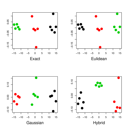
Figure 7: Example 1. The plots show pairwise distances as represented by multi-dimensional scaling. The plots show three clusters of five normal distribution each. All four methods are accurate.

Our second and third examples are chosen to illustrate that less clean clusters of data-sets cannot be well identified by the Gaussian approximation. Example 2 consists of two clusters. The first cluster has twenty normal distributions with mean $0$ and variance $1$. The second cluster has twenty distributions each of which has the form $(1/2)\delta_{-1}+(1/2)\delta_{1}$. This means that the first and second moments are also 0 and 1 so the Gaussian approximation should be unable to find the two clusters.

Figure 8 shows the distances computed with the Gaussian approximation and the Hybrid method, versus the Wasserstein procedure. The $45^{o}$ degree line is included for illustrating that the distances among distributions between the Gaussian approximation and the Wasserstein method are not close to each other, while the Hybrid and Wasserstein procedures displays similar distances. This plot complements the following Figure 9, showing the clustering obtained in this example, and illustrates that distances from the Gaussian approximation are a poor approxmation. Figure 9 shows indeed that, as expected, the Gaussian approximation does not work well.

Figure 8: Example 2. Plots of Gaussian and Hybrid distances of two data sets versus Wasserstein distance. The line across the plots is the $45^{o}$ line. The left hand side plot shows the distances among distriutions computed with the normal approximations are far from the Wasserstein distance.

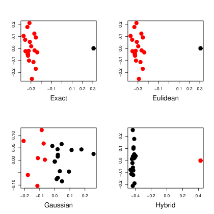
Figure 9: Example 2. While the Gaussian approximation does detect the two clusters, they are not well identified. The projection plots show random points in the plane. The other three methods, instead, identify the clusters correctly.

Our third example consists of three clusters of distributions, each being a mixture of normal distributions. This example also shows that the Gaussian approximation does not identify the clusters. As in Example 2, we first display the plots of the distances, in Figure 10, and then Figure 11 with plots of the multidimensional scaling projections. This confirms the issue noted earlier for the Gaussian approximation. Note that the clusters displayed in some plots are very close together and not easily detectable in the picture. But it is clear that the Gaussian approximation does not fare well.

Figure 10: Example 3. Plots of Gaussian and Hybrid distances of three data sets versus Wasserstain distance. The left hand side plot also shows distances among distriutions computed by the Gaussian approximations are far from the Wasserstein distance.

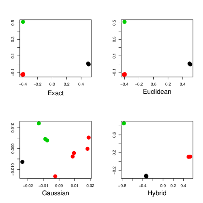
Figure 11: Example 3. Clusters for mixtures of Normal distributions. The Gaussian approximation does not performs well.

5.2 Multivariate Examples

In this section we consider three artificial data-sets in two dimensions. We no longer consider the exact Wasserstein method which is computationally prohibitive. We obtain, instead, clustering from the other three methods of Section 4. For each example, we will plot the parwise distances between datasets using multi-dimensional scaling.

The first example consists of $40$ bivariate Normal distributions, with $n=100$ observations each. Twenty of them have mean $0$ and variance $1$, the other twenty have meann $5$ and variance $1$. We also include twenty bivariate uniform distributions each with $100$ data points, for a total of three distributional clusters.

Figure 12 displays the boxplots of the first coordinates of the three data sets. The clusters appear to be well separated as expected. All three methods performs well, as it can be seen from the clusters obtained from the Euclidean, Normal, and Hybrid methods in Figure 13.

Figure 12: Boxplots of first coordinates in the bivariate example 1.

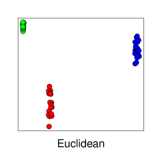
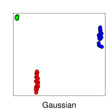
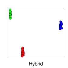
Figure 13: Bivariate Example 1. Clusters obtained using the procedures Gaussian and Hybrid.

The second example consists of four groups of distributions which are uniform on circles, each with $n=100$ data points. The circles’ centers and radii are randomly selected. More specifically the centers are generated from uniform distributions, with various ranges, as are their radii. Figure 14 displays the data that form four well separated clusters. Figure 15 shows the results for the three methods of clustering. All of them identify the four clusters correctly.

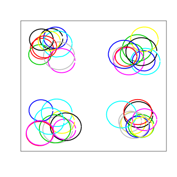
Figure 14: Bivariate Example 2. The datasets.

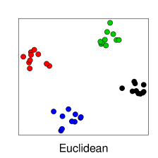
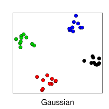
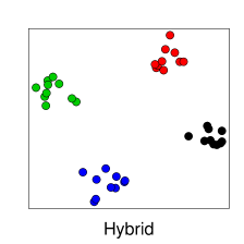
Figure 15: Bivariate Example 2. Clusters.

Our third example consists of two groups of distributions. One group of 50 distributions, withg 100 observations each, are uniformely distributed on a cirle and the 50 distributions in the other group are normal with mean $0$ and variance $1$. Figure 16 shows the boxplot of their first coordinates. Figure 17 presents the results for the three clustering methods. As expected the Gaussian procedure performs quite poorly.

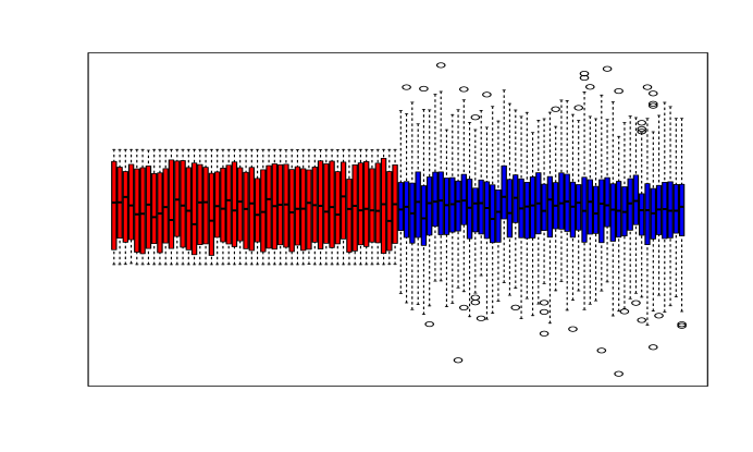
Figure 16: Bivariate Example 3. Boxplots of first coordinates.

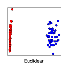
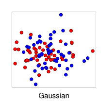
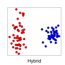
Figure 17: Bivariate Example 3. Clusters.

5.3 Multivariate Example: Cytometric Data

We now apply the Gaussian and Hybrid methods for clustering distributions, presented in Sections 3 and 4 to a collection of data sets from cytometric genetic research by Maier et al. (2007). The authors obtained fluorescence intensity measures of fluorophore-conjugated reagents on whole blood, stained with an antibody marker. The data record the luminosity of four proteins linked to the T-cells, that are part of the adaptive immune system. Luminosity was measured on the proteins SLP76, ZAP70, CD4, and CD45RA before and after stimulation with the antibody anti-CD3. Two sets of blood samples were collected. One sample consists in 13 four-dimension data-sets, stained prior to anti-CD3 stimulation. The second sample, of 30 more data-sets, stained five minutes after stimulation, for a total of 43 data-sets in four dimension. Figure 18 shows pairwise scatterplots for the first dataset.

Figure 18: Cytometric Data. Scatterplots of joint luminosity recorded for the first distribution of 13 blood samples stained prior to the anti-CD3 stimulation.

In this example, for reasons explained in Section 5.4, we searched for six clusters. Figure 19 and Figure 20 show the boxplots of the luminosity values recorded of the proteins, SLP76, and ZAP70 in the 43 data-sets.

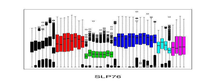
Figure 19: Cytometric Data. Boxplots of SLP76.

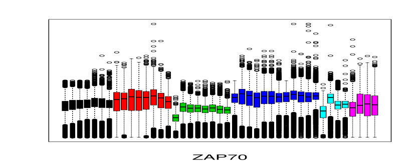
Figure 20: Cytometric Data. Boxplots of ZAP70.

The boxplots are color coded by our clustering. Note that the boxplots of the SLP6 and ZAP70 proteins correspond nicely to the six clusters. The third and fourth proteins , CD4, and CD45RA in Figure 20, instead do not seem to be well clustered. We conclude that the clustering information is deriving mainly from SLP6 and ZAP70.

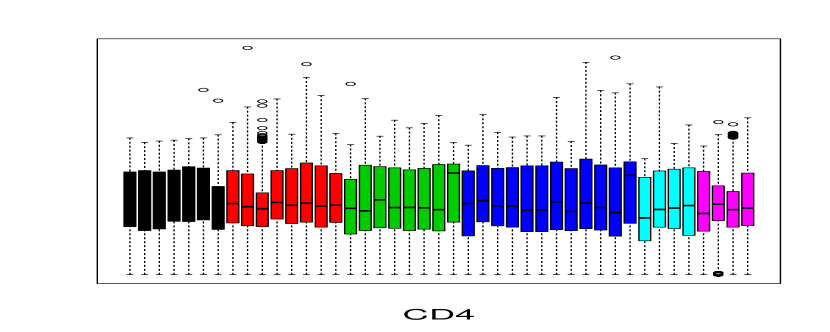
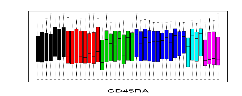
Figure 21: Cytometric Data. Boxplots of CD4 and CD45A.

The following Figure 22 shows the six clusters obtained with the Gaussian and the Hybrid procedures. Although the clusters appear to be not so well separated, we recall that multidimensional scaling projections from several dimensions to two might not be very accurate. Our choice, in searching for six clusters, has been suggested by the plots in Figure 24 of Section 5.4, where the issue of choosing the number of clusters is examined, and reinforced by the boxplots in Figure 19 and Figure 20

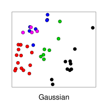
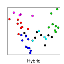
Figure 22: Cytometric Data. Clusters Clusters obtained using the procedures Gaussian and Hybrid.

5.4 Choosing $k$: Elbows

The issue of choosing $k$ in $k$-means clustering is a well-studied problem. Perhaps the oldest and simplest method is to plot the sums of squares versus $k$ and look for an elbow. For distribution clustering, we plot $S_{k}=\sum_{j}\sum_{s\in{\cal C}_{j}}W^{2}(P_{s},c_{j})$ versus $k$. In some cases, the elbow is clearer if we plot $1/S_{k}$ versus $k$. Figure 23 shows the plot of $S_{k}$ versus $k$ for the second example in Section 5.2 where data were generated as four groups of circles. We see a clear elbow at $k=4$. Figure 24 shows another plot of cluster quality versus $k$. In this case, for the cytometric data sets, we plot $1/\sum_{j}\sum_{s\in{\cal C}_{j}}W^{2}(P_{s},c_{j})$ as the inverse plot shows a clearer signal. The elbow is at $k=6$.

Figure 23: Plot of $\sum_{j=1}^{k}\sum_{s\in{\cal C}_{j}}W^{2}(P_{s},c_{j})$ for $k=1,\ldots,10$ for the example with four groups of circles. Note the pronounced elbow at $k=4$.

Figure 24: Plot of $1/\sum_{j=1}^{k}\sum_{s\in{\cal C}_{j}}W^{2}(P_{s},c_{j})$ for $k=1,\ldots,9$ for the cytometric data. Note the elbow at $k=6$.

5.5 The Pre-testing Speedup

We generated 100 observations from each of 30 multivariate Normal distributions that lie in three distinct groups. After computing the rescaled data $\widetilde{X}$, we apply the cross-match test from Rosenbaum (2005) to see if the rescaled data differ significantly from the sample from the reference distribution. We used level $\alpha=0.10$. In the majority of cases, the test does not reject and we set $\psi_{j}=0$ which saves considerable computing time. Typically, the clustering is perfect (adjusted Rand index of 1). But when the same procedure is applied to the Normal and circles data, the null is almost always rejected (as expected) and we need to do the full computations.

6 Other Clustering Methods

There are, of course, many other clustering methods besides $k$-means clustering. In this section we give a sense of how the hybrid distance can be used for two other clustering methods.

Hierarchical Clustering. The hybrid distance can easily be used for hierarchical clustering. These are the steps for single linkage hierarchical clustering:

1. Compute the transform $(\mu_{j},\Sigma_{j},\psi_{j})=\phi(P_{j})$ for each distribution.

2. Compute the pairwise distances $H_{jk}=H(P_{j},P_{k})$.

3. Find the pair $(j,k)$ that minimizes $H_{j,k}$. Merge $P_{j}$ and $P_{k}$ into a single distribution $P_{jk}=\pi P_{j}+(1-\pi)P_{k}$ where $\pi=n_{j}/(n_{j}+n_{k})$ and $n_{j}$ and $n_{k}$ are the sample sizes of the two datasets.

4. Compute the representation $(\mu_{jk},\Sigma_{jk},\psi_{jk})$ of $P_{jk}$ by computing the barycenter of $P_{j}$ and $P_{k}$ with weights $\pi_{jk}$ and $1-\pi_{jk}$.

5. Repeat steps 2-4 until all distributions are merged.

By working with the hybrid representations we do not have to keep recomputing Wasserstein distances.

Mean-Shift and Medioid-Shift Clustering. Next we discuss mean shift clustering and medioid shift clustering (Cheng, 1995; Chacón and Duong, 2018; Jiang et al., 2018; Chacón et al., 2015). First we review these methods when applied to a single dataset. Give a sample $Y_{1},\ldots,Y_{n}$ from a distribution $P$ with density $p$, mean shift clustering works by first computing an estimate $\widehat{p}$ of $p$. Let $m_{1},\ldots,m_{k}$ be the modes of $\widehat{p}$. Given any point $y$, if we follow the gradient of $\widehat{p}$ starting at $y$ we will end up at one of the modes. In this way the modes define a partition of the sample space. This partition defined the mode-based clustering. There is a simple iterative algorithm called the mean-shift algorithm to implement this idea. Recently, Duong et al. (2016) showed that if we use $r$-nearest neighnor density estimation, then the iterative algorithm takes the following form. Pick any starting value $x$. Define $y^{(0)},y^{(1)},\ldots$ by $y^{(0)}=y$ and

$$y^{(s)}=\frac{1}{r}\sum_{N_{r}(y^{(s-1)})}Y_{i}$$

where $N_{r}(y)$ denotes the $r$-nearest neighbors of the point $y$. This iteration leads to a mode of the estimated density. This assigns any point $y$ to a mode. The iteration can be applied to any set of starting points although these starting points are usually taken to be the data points.

Returning to distribution clustering, we have a set of distributions $P_{1},\ldots,P_{N}$ which we now regard as a sample from a measure $\Pi$ on the space of distributions. Unfortunately, $\Pi$ does not have a density in any meaningful sense. Nonetheless, we can formally apply the mean shift clustering algorithm. Given any $P$, let $N_{r}(P)$ denote the $r$ closest distributions in $\{P_{1},\ldots,P_{N}\}$ to $P$ under the hybrid distance. Let ${\rm Bary}(N_{r}(P))$ denote the hybrid barycenter of the distributions in ${\rm Bary}(N_{r}(P))$. We then define $P^{(0)}=P$ and

$$P^{(s)}={\rm Bary}(N_{r}(P^{(s-1)})).$$

A faster approach, which avoids computing the barycenter, is mediod-shift clustering. In this case, we begin by estimating $\rho(P_{j})=1/d(P,P_{r}(P))$ where $P_{r}(P)$ is the $r^{\rm th}$ nearest neighbor. This can be thought of as a pseudo-density. We move $P$ to the distribution in $N_{r}(P)$ with highest pseudo-density. This is repeated until there is no change. This can be regarded as an approximation to mean-shift clustering.

As an example, we consider a collection of 80, two-dimensional datasets. Each dataset has $n=100$ observations from a bivariate Normal. We construct the data so that there are four, well-defined clusters. Figure 25 shows mediod-shift clustering using the hybrid distance. The plots correspond to $r=2,10,15$ and 20 nearest neighbors. The plots show the MDS of the data sets and the paths of the data as the clustering proceeds. The red dots show the final destinations, that is, the pseudo-modes. When $r=2$ we get extra clusters. When $r$ reaches 20 we start to oversmooth and end up with 2 clusters. There is a large range of values of $r$ that lead to the correct answer of 4 clusters.

Currently, we do not have a theoretical basis for applying the mean shift algorithm to distributions. We believe that it may be possible to define a pseudo-density on the space of distributions simialr to the approach used by In the context of clustering functional data, Ferraty and Vieu (2006) justify density clustering by defining a pseudo-density. We conjecture that density clustering in Wasserstein space can be similarly justified by regarding the density estimator as estimating a pseudo-density. For example, if $P$ is a random distribution, one can define the pseudo-density at $P_{0}$ by $\mathbb{P}(P\in B(P_{0},h))$ where $B(P_{0},h)=\{P:\ H(P_{0},P)\leq h\}$. We leave the details for future work.

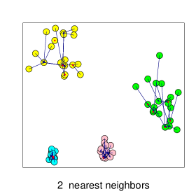
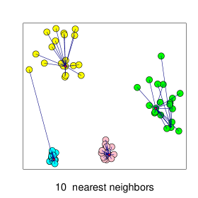
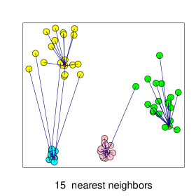
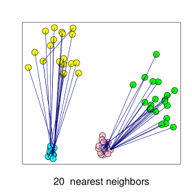
Figure 25: Mediod-Shift Clustering using the hybrid distance. The plots show the MDS of the data sets and the paths of the data as the clustering proceeds for$r=2,10,15$ and 20 nearest neighbors.

7 Other Hybridizations

Now we consider other hybrid distances of the form,

$$H^{2}(X,Y)=W^{2}(Z_{X},Z_{Y})+W_{\dagger}^{2}(\widetilde{X},\widetilde{Y})$$

where we explore other choices besides the tangent distance for $W_{\dagger}$. In each case, we want an approximate distance that can be computed quickly.

Marginal Distance. Here we take

$$W_{\dagger}^{2}(X,Y)=\sum_{j=1}^{d}W^{2}(X(j),Y(j))$$

where $X(j)$ and $Y(j)$ are the $j^{\rm th}$ components of $X$ and $Y$. It then follows that

$$W_{\dagger}^{2}(X,Y)=\sum_{j=1}^{d}\int_{0}^{1}|F^{-1}_{j}(u)-G^{-1}_{j}(u)|^{2}du$$

where $F_{j}(t)=P(X(j)\leq t)$ and $G_{j}(t)=Q(Y(j)\leq t)$. Hence,

$$H^{2}(X,Y)=||\mu_{X}-\mu_{Y}||^{2}+{\rm B}^{2}(\Sigma_{X},\Sigma_{Y})+\sum_{j=1}^{d}\int_{0}^{1}|F^{-1}_{j}(u)-G^{-1}_{j}(u)|^{2}du.$$

The estimate is

$$\widehat{H}^{2}(X,Y)=||\widehat{\mu}_{X}-\widehat{\mu}_{Y}||^{2}+{\rm B}^{2}(\widehat{\Sigma}_{X},\widehat{\Sigma}_{Y})+\sum_{j=1}^{d}\int_{0}^{1}|\widehat{F}^{-1}_{j}(u)-\widehat{G}^{-1}_{j}(u)|^{2}du.$$

Assuming we have samples $m$ observations from each dataset, we have the further simplification that

$$\int_{0}^{1}|\widehat{F}^{-1}_{j}(u)-\widehat{G}^{-1}_{j}(u)|^{2}du=\frac{1}{m}\sum_{i}(X_{(i)}(j)-Y_{(i)}(j))^{2}$$

where $X_{(1)}(j),\ldots,X_{(n)}(j)$ and $Y_{(1)}(j),\ldots,Y_{(n)}(j)$ are the order statistics for the $j^{\rm th}$ coordinate of $X$ and $Y$, respectively.

Next we consider an example. We generate 100 datasets. The first 50 are standard bivariate Normal. The second 50 are uniform on a circle, scaled to have the same mean and covariance as the Normal.The left plot of Figure 26 shows the Gaussian-Wasserstein distances using multidimensional scaling. The colors indicate Normal (black) and circular (red). The Gaussian-Wasserstein distance cannot distinguish the two types of datasets. The right plot shows the marginal hybrid distance. Here, the two types of datasets are clearly distinguished.

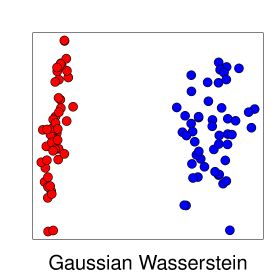
Figure 26: There are 100 distributions. The first 50 are standard bivariate Normal. The second 50 are uniform on a circle, scaled to have the same mean and covariance as the Normal. The left plot shows the Gaussian-Wasserstein distance. The colors indicate the Normal data (red) and the circular (blue). As expected, the Gaussian-Wasserstein distance cannot distinguish the two types of datasets. The right plot shows the marginal hybrid distance. Here, the two types of datasets are clearly distinguished.

Transformed Gaussian Approximation. Recall that the Gaussian-Wasserstein distance is

$$G^{2}(X,Y)=||\mu_{X}-\mu_{Y}||^{2}+B^{2}(\Sigma_{X},\Sigma_{Y}).$$

A hybrid distance that leverages the simplicity of $G$ can be obtained by repeatedly applying a nonlinear transformation to the variables, using the $G$, standardizing the variables and repeating. Let $L$ be the map that takes $X$ to $\widetilde{X}=\Sigma_{X}^{-1/2}(X-\mu_{X})$ and let $\Phi$ be some fixed nonlinear map. Define $H^{2}(X,Y)=G^{2}(X,Y)+W_{\dagger}(X,Y)$ where

$$W_{\dagger}(X,Y)=\sum_{j=1}^{k}G^{2}(X_{j},Y_{j})$$

with

$$X_{j}=\underbrace{[(\Phi\circ L)\circ\cdots(\Phi\circ L)]}_{k\ {\rm times}}X,\ \ \ Y_{j}=\underbrace{[(\Phi\circ L)\circ\cdots(\Phi\circ L)]}_{k\ {\rm times}}Y.$$

In the case $k=1$ this simplifies to

$$H^{2}(X,Y) =G^{2}(X,Y)+G^{2}(\Phi(\widetilde{X}),\Phi(\widetilde{Y}))$$

$$=||\mu_{X}-\mu_{Y}||^{2}+B^{2}(\Sigma_{X},\Sigma_{Y})+||\mu_{\Phi(\widetilde{X})}-\mu_{\Phi(\widetilde{Y})}||^{2}+B^{2}(\Sigma_{\Phi(\widetilde{X})},\Sigma_{\Phi(\widetilde{Y})})$$

There are many possible choices for $\Phi$. The only requirement is that $\Phi$ be non-linear otherwise the transformation adds no information beyond that already captured by $G$. A convenient choice is the polynomial transform

$$\Phi(x)=([x]_{2},\ldots,[x]_{k})$$

where $[x]_{2}=(x_{i_{1}}x_{i_{2}}:\ 1\leq i_{1}\leq i_{2}\leq d)$, $[x]_{3}=(x_{i_{1}}x_{i_{2}}x_{i_{3}}:\ 1\leq i_{1}\leq i_{2}\leq i_{3}\leq d)$, etc.

As an example, consider a one-dimensional case. We suppose that $P_{1},\ldots,P_{50}=N(0,1)$ and $P_{j}=(1/2)\delta_{-1}+(1/2)\delta_{1}$ for $j=51,\ldots,100$. We take $\Phi(X)=(X^{2},X^{3},X^{4})$. Since the first two moments of all the distributions match, the Gaussian distance is unable to distinguish the 100 distributions. Figure 27 shows the pairwise distances using multidimensional scaling (MDS). The top left plot is based on parwise Wasserstein distances. The two groups are clearly visible. The top rightplot used Gaussian Wasserstein distance. As expected, the distributions are mixed up. The bottom left uses hybrid distance with polynomial transformation. Here we see that again, the distributions are clearly separated.

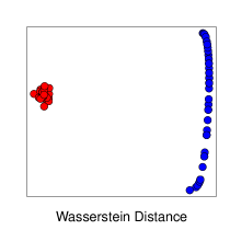
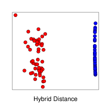
Figure 27: 50 distributions are N(0,1) (black) and 50 are mixtures of the form $\delta_{-1}+(1/2)\delta_{1}$ (red). The sample size for each distribution is 1,000. Left: MDS based on parwise Wasserstein distance. The two groups are clearly visible. Middle: MDS based on the Gaussian Wasserstein distance. As expected, the mixtures distributions are mixed in with the Normals. Right: Hybrid distance with polynomial transformation. Here we see that again, the distributions are clearly separated.

8 Discussion

We have proposed a modified version of the Wasserstein distance called the hybrid distance that can be used for clustering sets of distributions. The distances and the barycenter can be computed quickly. The slowest part of the computation is finding the optimal matching permutation which takes $O(m^{3})$ operations. There is large literature on approximate matching in the computer science literature. It would be interesting to incorporate some of those methods to further speed up the computations.

The hybrid distance can be used for other tasks as well such as shrinkage estimation, modeling random effects, domain adaptation, and image processing. We will report on these applications in future work. We conclude by discussing a few issues.

8.1 Energy Distance

The energy distance (Székely and Rizzo (2013)) is another metric that takes the underlying geometry of the sample space into account. The metric defined by

$${\cal E}(X,Y)\equiv{\cal E}(P,Q)=2\mathbb{E}||X-Y||-\mathbb{E}||X-X^{\prime}||-\mathbb{E}||Y-Y^{\prime}||$$ (13)

where $X,X^{\prime}\sim P$ and $Y,Y^{\prime}\sim Q$. The energy distance has many of the desirable properties that the Wasserstein distance has including the ability to compare discrete and continuous distributions.

A sample estimator of the distance based on $X_{1},\ldots,X_{n}\sim P$ and $Y_{1},\ldots,Y_{m}\sim Q$ is

$$\widehat{\cal E}(X,Y)=\frac{2}{nm}\sum_{i,j}||X_{i}-Y_{j}||-\binom{n}{2}\sum_{i\neq j}||X_{i}-X_{j}||-\binom{m}{2}\sum_{i\neq j}||Y_{i}-Y_{j}||.$$ (14)

In fact, there are very fast approximations that speed up the calculations; see Huang and Huo (2017).

To the best of our knowledge, there is no fast way to compute barycenters with this metric. But we can get around this by using $k$-mediods in place of $k$-means. This, if $P_{1},\ldots,P_{r}$ is a set of distributions in a cluster, we define the centroid to be $P_{t}$ where $P_{t}=\operatorname*{argmin}_{1\leq j\leq r}\sum_{s}{\cal E}(P_{j},P_{s})$. That is, we restrict the search for a centroid to be over the observed distributions.

Hence, if we use $k$-mediods, distribution clustering with the energy distance is feasible. However, the energy distance is not shape preserving. To see this, consider the following example. $P_{1}=\delta_{-a}$ and $P_{2}=\delta_{a}$ where $a>0$ and $\delta$ denotes a point mass. The barycenter $P$ minimizes ${\cal E}(P,P_{1})+{\cal E}(P,P_{2})$. Recall the the Wasserstein barycenter is $\delta_{0}$. But this is not true for the energy distance. To see this, consider distributions of the form $P=(1/2)\delta_{-b}+m(1/2)\delta_{b}$. It is easy to show that, over such distributions, ${\cal E}(P,P_{1})+{\cal E}(P,P_{2})$ is minimized by choosing the mixture $P=(1/2)\delta_{-a}+m(1/2)\delta_{a}$. This implies that the barycenter cannot be $\delta_{0}$ as desired.

In summary, we see that when distributions are well separated, the energy barycenter is over-dispersed compared to the Wasserstein barycenter. This leads to situations where the centroid of a cluster might look quite different than the distributions in the cluster. It is tempting to look for a simple modification of the energy distance that fixes this problem. We have tried several approaches without success. Thus, the advantage of energy distance is that it can be computed quickly but the disadvantage is that it does not preserve the shape of the distributions when computing barycenters.

8.2 Optimal Preconditioning

The linear transformation that we used, namely, $\widetilde{X}=\Sigma_{X}^{-1/2}(X-\mu_{X})$ matches the first two moments of $\widetilde{X}$ with $U$ where $U\sim R$ is the reference distribution. This transformation is chosen for convenience. An alternative approach is to choose an optimal linear transformation. That is, we could choose $a$ and $A$ to minimize $W^{2}(a+AX,U)$. Unfortunately, computing the optimal $a$ and $A$ is non-trivial. If we permit linear transformations of both $X_{j}$ and $U$ then there is a closed form expression for the optimal transformation; see Kuang and Tabak (2017). This requires a different transformation of $U$ for each $X_{j}$. Hence, we lose the idea of a single, fixed, reference distribution. It would be possible to construct a composition of maps $X_{j}\to\widetilde{X}_{j}\to\widetilde{Z}_{j}\to U$ where $X_{j}\to\widetilde{X}_{j}$ is the optimal linear map on $X_{j}$ and $\widetilde{Z}_{j}\to U$ is the optimal linear map for $U$. Kuang and Tabak (2017) show that the optimal map $T(X)$ is the same as the composition $M^{-1}\circ T_{\dagger}\circ L$ where $T_{\dagger}$ is the optimal transport map from $\widetilde{X}$ to $\widetilde{Y}$; see Figures 28 and 29.

Figure 28: The optimal linear map, preserves the Wasserstein distnce and makes $\widetilde{X}$ and $\widetilde{Y}$ as close as possible.

Figure 29: The optimal linear preconditioning is applied to $X_{j}$ and $U$ in a pairwise fashion.

This might lead to more accurate approximations at the expense of much more computation. In the interest of keeping the method as simple as possible, we have not use this more involved approach.

8.3 The Choice of Reference Measure and Multiple Tangents

When we used the tangent approximation, we approximated the distance by projecting one a single tangent space. An alternative, when there are a large number of diverse distributions, is to use several tangent approximations. The datasets could first clustered using some fast approximation, such as the marginal hybrid distance. A separate tangent approximation is computed for each perliminary cluster. Then each distribution can be represented by its local tangent approximation using the same reference measure. Another issue is the choice of reference measures. We do not know if there is an optimal reference measure. It is not even clear how to define such a notion of optimality. We conjecture that, at least for distribution clustering, the choice of reference measure is not critical.

8.4 Other Applications of the Hybrid Approach

The hybrid distance can be used for other tasks besides clustering. In this section we outline how the hybrid distance can be used for these tasks.

Nonparametric Shrinkage. Suppose that $P_{1},\ldots,P_{N}$ are random distributions drawn from a distribution $\Pi$. Let ${\cal D}_{j}$ be $n_{j}$ samples drawn from $P_{j}$. Suppose that we want to borrow strength from all the data to estimate each $P_{j}$. Let $R$ be a reference measure and let $(\mu_{j},\Sigma_{j},\psi_{j})=\phi(P_{j})$ denote the hybrid transform as in (12). Let $(\widehat{\mu}_{j},\widehat{\Sigma}_{j},\widehat{\psi}_{j})$ denote the $j^{\rm th}$ estimate. We can apply shrinkage estimation separately to the $\widehat{\mu}_{j}$’s, the $\widehat{\Sigma}_{j}$’s and the $\widehat{\psi}_{j}$’s. Denote these estimates by $\overline{\mu}_{j}$, $\overline{\Sigma}_{j}$, $\overline{\psi}_{j}$. Inverting $\phi$ gives the shrinkage estimator $\overline{P}_{j}$. We obtain $\overline{\mu}_{j}$ using standard James-Stein shrinkage, $\overline{\Sigma}_{j}$ by covariance shrinkage as in Nguyen et al. (2018) and $\overline{\psi}_{j}$ is obtained by functional shrinkage as in Guo (2002).

Multi-Sample Testing. Suppose that we want to test the null hypothesis $H_{0}:P_{1}=\cdots=P_{N}$. The hybrid distance allows us to split this null into three different null hypotheses, namely, $H_{0}:\mu_{1}=\cdots=\mu_{N}$, $H_{0}:\Sigma_{1}=\cdots=\Sigma_{N}$ and $H_{0}:\psi_{1}=\cdots=\psi_{N}$. This allows us to separate the deviations from the null in terms of location, scale and shape.

Multi-Level Clustering. After clustering the distributions $P_{1},\ldots,P_{N}$ into clusters ${\cal C}_{1},\ldots,{\cal C}_{k}$, we may want to further cluster the datasets ${\cal D}_{1},\ldots,{\cal D}_{N}$. We could apply any standard clustering algorithm to each dataset. But we may want the distributions in a cluster ${\cal C}_{j}$ to have similar clusterings. For example, we could use Normal mixture clustering on each dataset then apply the shrinkage ideas mentioned above to make the clusterings similar. This is an alternative to simultaneous Wasserstein clustering as in Ho et al. (2017) which is quite expensive.

Appendix

Consistency. In this section we show that the 1-nearest neighbor regression method for estimating the transport map is consistent. Let $X_{1},\ldots,X_{m}\sim P$ and $Y_{1},\ldots,Y_{m}\sim Q$. Assume that $P$ has density $p$ and $Q$ has density $q$ and that both are supported on a compact subset of $\mathbb{R}^{d}$. Let $T$ be the optimal transport map from $P$ to $Q$. Let $P_{n}$ be the empirical measure based on $X_{1},\ldots,X_{m}$ and let $Q_{n}$ be the empirical measure based on $Y_{1},\ldots,Y_{m}$.

Let $V_{1},\ldots,V_{m}$ denote the Voronoi tesselation defined by $X_{1},\ldots,X_{m}$. Let $\pi$ be the permutation that minimizes

$$\sum_{i}||X_{i}-Y_{\pi(i)}||^{2}.$$

Our estimator of $T$ is

$$\widehat{T}(x)=\sum_{s=1}^{j}I(x\in V_{s})Y_{\pi(j(x))}$$ (15)

where $j(x)$ is the integer $j$ such that $||x-X_{j}||\leq||x-X_{t}||$ for all $t\neq j$.

Theorem 3

Let $P$ and $Q$ be supported on a compact set ${\cal X}\subset\mathbb{R}^{d}$. Suppose that $P$ and $Q$ have continuous densities $p$ and $q$ and that $\inf_{x\in{\cal X}}p(x)>0$ and $\inf_{y\in{\cal Y}}q(x)>0$. Let $X_{1},\ldots,X_{n}\sim P$ and $Y_{1},\ldots,Y_{n}\sim Q$. Let $T$ be the optimal transport map and let $\widehat{T}$ be the estimated map in (15). Then

$$\int||x-\widehat{T}(x)||^{2}dP(x)=\int||x-T(x)||^{2}dP(x)+O_{P}(\log n\,n^{-1/d})$$

for some positive constant $a>0$.

Proof. Let $V_{1},\ldots,V_{n}$ denote the Voronoi diagram defined by $X_{1},\ldots,X_{n}$. From Lemma 4 below, $\max_{j}|P(V_{j})-1/n|+O_{P}(1/n^{2})$ and $\max_{j}{\rm diam}(V_{j})=O_{P}(\log n\,n^{-1/d})$.

Let $P_{n}$ and $Q_{n}$ be the empirical distributions of $X_{1},\ldots,X_{n}$ and $Y_{1},\ldots,Y_{n}$. From Weed and Bach (2017), we have that $W^{2}(P_{n},Q_{n})=O_{P}(n^{-2/d})$. Now

$$\int||x-\widehat{T}(x)||^{2}dP(x) =\sum_{j}\int_{V_{j}}||x-\widehat{T}(x)||^{2}dP(x)=\sum_{j}\int_{V_{j}}||x-\widehat{T}(X_{j})||^{2}dP(x)$$

$$=A+B+C$$

where

$$A=\sum_{j}\int_{V_{j}}||x-X_{j}||^{2}dP(x),\ B=\sum_{j}\int_{V_{j}}||X_{j}-\widehat{T}(X_{j})||^{2},\ C=\sum_{j}\int_{V_{j}}\langle x-X_{j},X_{j}-\widehat{T}(X_{j})\rangle dP(x).$$

Now $A\leq\sum_{j}\max_{j}{\rm diam}(V_{j})P(V_{j})=\max_{j}{\rm diam}(V_{j})=O_{P}(\log n\,n^{-1/d})$

$$B =\sum_{j}||X_{j}-\widehat{T}(X_{j})||^{2}P(V_{j})=\frac{1}{n}\sum_{j}||X_{j}-\widehat{T}(X_{j})||^{2}+\sum_{j}||X_{j}-\widehat{T}(X_{j})||^{2}(P(V_{j})-1/n)$$

$$=W^{2}(P_{n},Q_{n})+\sum_{j}||X_{j}-\widehat{T}(X_{j})||^{2}(P(V_{j})-1/n)$$

$$=W^{2}(P_{n},Q_{n})+O_{P}(1/n^{2})=W^{2}(P,Q)+O_{P}(1/n^{2})+O_{P}(n^{-2/d})$$

$$=\int||x-T(x)||^{2}dP(x)+O_{P}(n^{-2/d})$$

and

$$C =\sum_{j}\int_{V_{j}}\langle x-X_{j},X_{j}-\widehat{T}(X_{j})\rangle dP(x)\leq\sum_{j}\sqrt{\int_{V_{j}}||x-X_{j}||^{2}}dP(x)\sum_{j}\sqrt{||X_{j}-\widehat{T}(X_{j})||^{2}dP(x)}$$

$$=O(\max_{j}{\rm diam}(V_{j}))=O_{P}(\log n\,n^{-1/d}).$$

$\Box$

The following are standard facts about Voronoi cells for strictly positive densities.

Lemma 4

Suppose that $P$ is supported on a compact set and has continous density $p$ that is strictly bounded away from 0. Let $X_{1},\ldots,X_{n}\sim P$ and let $V_{1},\ldots,V_{n}$ be the Voronoi cells defined by $X_{1},\ldots,X_{n}$. Then (i) $\mathbb{E}[P(V_{i})]=1/n$, (ii) ${\rm Var}[P(V_{i})]\leq 2/n^{2}$ and (iii) $\max_{j}{\rm diam}(V_{j})=O_{P}(\log n\,n^{-1/d})$, (iv) $\sum_{i}|P(V_{i})-1/n|=o_{P}(1)$.

Wasserstein $k$-means in one dimension. Now we give the steps for exact Wasserstein $k$-means clustering in one dimension. Given datasets ${\cal D}_{1},\ldots,{\cal D}_{N}$ let $F_{1},\ldots,F_{N}$ be the empirical cdf’s. We use the trimmed Wasserstein distance

$$W^{2}(F_{j},F_{k})=\frac{1}{1-2\delta}\int_{\delta}^{1-\delta}(F_{j}^{-1}(s)-F_{k}^{-1}(s))^{2}ds$$

where $\delta>0$ is some specified positive trimming constant.

First, we use $k-{\rm means}^{++}$ seeding to get starting centroids:

 
Wasserstein $k$-means seeding
 

1. Input: integer $k$ and data sets ${\cal D}_{1},\ldots,{\cal D}_{N}$.

2. Compute all parwise Wasserstein distances

   $$D_{jk}^{2}=W^{2}(F_{j},F_{k}).$$

3. Let $F_{1},\ldots,F_{N}$ be the empirical cdf’s of the data sets.

4. Find the starting values:

   1. Let $c_{1}=F_{j}$ where $j$ is chosen randomly from $1,\ldots,N$. Set ${\cal C}=\{j\}$.

   2. Choose $c_{2}$ randomly from $\{F_{1},\ldots,F_{N}\}$ where $F_{s}$ is chosen with probability proportional to $\min_{j\in{\cal C}}D_{sj}^{2}$.

   3. Set ${\cal C}\leftarrow{\cal C}\bigcup\{j\}$.

   4. Repeat the last two steps until ${\cal C}=\{c_{1},\ldots,c_{k}\}$ has $k$ elements.

The main algorithm is as follows.

 
Wasserstein $k$-means
 

1. Run Wasserstein $k$-means seeding to get centroids ${\cal C}$.

2. Compute $D_{js}=W(F_{j},c_{s})$ for $j=1,\ldots,N$ and $s=1,\ldots,k$.

3. Assign each $F_{j}$ to its nearest centroid: let ${\cal C}_{j}=\{F_{r}:\ W(F_{r},F_{j})<W(F_{r},F_{t})\ t\neq j\}$.

4. Let $c_{j}$ be the centroid of ${\cal C}_{j}$ using Wasserstein centroid.

5. Repeat last two steps until convergence.

 
Wasserstein centroid
 

1. Given one-dimensional cdf’s $F_{1},\ldots,F_{N}$.

2. Let $c(s)=\frac{1}{N}\sum_{j}F_{j}^{-1}(s).$

3. Return $F(x)=c^{-1}(x)$.

References

• รlvarez-Esteban etย al. (2016) Pedroย C รlvarez-Esteban, Eย del Barrio, JAย Cuesta-Albertos, and Cย Matrรกn. A fixed-point approach to barycenters in Wasserstein space. Journal of Mathematical Analysis and Applications, 441(2):744โ€“762, 2016.
• Arthur and Vassilvitskii (2007) David Arthur and Sergei Vassilvitskii. k-means++: The advantages of careful seeding. In Proceedings of the eighteenth annual ACM-SIAM symposium on Discrete algorithms, pages 1027โ€“1035. Society for Industrial and Applied Mathematics, 2007.
• Bhatia etย al. (2018) Rajendra Bhatia, Tanvi Jain, and Yongdo Lim. On the buresโ€“Wasserstein distance between positive definite matrices. Expositiones Mathematicae, 2018.
• Chacรณn and Duong (2018) Josรฉย E Chacรณn and Tarn Duong. Multivariate Kernel Smoothing and Its Applications. Chapman and Hall/CRC, 2018.
• Chacรณn etย al. (2015) Josรฉย E Chacรณn etย al. A population background for nonparametric density-based clustering. Statistical Science, 30(4):518โ€“532, 2015.
• Cheng (1995) Yizong Cheng. Mean shift, mode seeking, and clustering. IEEE transactions on pattern analysis and machine intelligence, 17(8):790โ€“799, 1995.
• del Barrio etย al. (2017) Eย del Barrio, JAย Cuesta-Albertos, Cย Matrรกn, and Aย Mayo-รscar. Robust clustering tools based on optimal transportation. Statistics and Computing, pages 1โ€“22, 2017.
• Duong etย al. (2016) Tarn Duong, Gaรซl Beck, Hanene Azzag, and Mustapha Lebbah. Nearest neighbour estimators of density derivatives, with application to mean shift clustering. Pattern Recognition Letters, 80:224โ€“230, 2016.
• Ferraty and Vieu (2006) Frรฉdรฉric Ferraty and Philippe Vieu. Nonparametric functional data analysis: theory and practice. Springer Science & Business Media, 2006.
• Givens etย al. (1984) Clarkย R Givens, Raeย Michael Shortt, etย al. A class of Wasserstein metrics for probability distributions. The Michigan Mathematical Journal, 31(2):231โ€“240, 1984.
• Guo (2002) Wensheng Guo. Functional mixed effects models. Biometrics, 58(1):121โ€“128, 2002.
• Ho etย al. (2017) Nhat Ho, XuanLong Nguyen, Mikhail Yurochkin, Hungย Hai Bui, Viet Huynh, and Dinh Phung. Multilevel clustering via Wasserstein means. arXiv preprint arXiv:1706.03883, 2017.
• Huang and Huo (2017) Cheng Huang and Xiaoming Huo. An efficient and distribution-free two-sample test based on energy statistics and random projections. arXiv preprint arXiv:1707.04602, 2017.
• Jiang etย al. (2018) Heinrich Jiang, Jennifer Jang, and Samory Kpotufe. Quickshift++: Provably good initializations for sample-based mean shift. arXiv preprint arXiv:1805.07909, 2018.
• Kuang and Tabak (2017) Max Kuang and Estebanย G Tabak. Preconditioning of optimal transport. SIAM Journal on Scientific Computing, 39(4):A1793โ€“A1810, 2017.
• Kuhn (1955) Haroldย W Kuhn. The hungarian method for the assignment problem. Naval research logistics quarterly, 2(1-2):83โ€“97, 1955.
• Maier etย al. (2007) Lisaย M Maier, Davidย E Anderson, Philipย L Deย Jager, Lindaย S Wicker, and Davidย A Hafler. Allelic variant in ctla4 alters t cell phosphorylation patterns. Proceedings of the National Academy of Sciences, 104(47):18607โ€“18612, 2007.
• Nguyen etย al. (2018) Vietย Anh Nguyen, Daniel Kuhn, and Peymanย Mohajerin Esfahani. Distributionally robust inverse covariance estimation: The Wasserstein shrinkage estimator. arXiv preprint arXiv:1805.07194, 2018.
• Panaretos and Zemel (2018) Victorย M Panaretos and Yoav Zemel. Statistical aspects of wasserstein distances. Annual Review of Statistics and Its Application, 2018.
• Rippl etย al. (2016) Thomas Rippl, Axel Munk, and Anja Sturm. Limit laws of the empirical Wasserstein distance: Gaussian distributions. Journal of Multivariate Analysis, 151:90โ€“109, 2016.
• Rosenbaum (2005) Paulย R Rosenbaum. An exact distribution-free test comparing two multivariate distributions based on adjacency. Journal of the Royal Statistical Society: Series B (Statistical Methodology), 67(4):515โ€“530, 2005.
• Silverman (2018) Bernardย W Silverman. Density estimation for statistics and data analysis. Routledge, 2018.
• Sommerfeld and Munk (2018) Max Sommerfeld and Axel Munk. Inference for empirical Wasserstein distances on finite spaces. Journal of the Royal Statistical Society: Series B (Statistical Methodology), 80(1):219โ€“238, 2018.
• Sommerfeld etย al. (2018) Max Sommerfeld, Jรถrn Schrieber, and Axel Munk. Optimal transport: Fast probabilistic approximation with exact solvers. arXiv preprint arXiv:1802.05570, 2018.
• Szรฉkely and Rizzo (2013) Gรกborย J Szรฉkely and Mariaย L Rizzo. Energy statistics: A class of statistics based on distances. Journal of statistical planning and inference, 143(8):1249โ€“1272, 2013.
• Villani (2003) Cรฉdric Villani. Topics in optimal transportation. American Mathematical Soc., 2003.
• Wang etย al. (2013) Wei Wang, Dejan Slepฤev, Saurav Basu, Johnย A Ozolek, and Gustavoย K Rohde. A linear optimal transportation framework for quantifying and visualizing variations in sets of images. International journal of computer vision, 101(2):254โ€“269, 2013.
• Weed and Bach (2017) Jonathan Weed and Francis Bach. Sharp asymptotic and finite-sample rates of convergence of empirical measures in Wasserstein distance. arXiv preprint arXiv:1707.00087, 2017.