Answering Range Queries Under Local Differential Privacy

Abstract.

Counting the fraction of a population having an input within a specified interval i.e. a range query, is a fundamental data analysis primitive. Range queries can also be used to compute other interesting statistics such as quantiles, and to build prediction models. However, frequently the data is subject to privacy concerns when it is drawn from individuals, and relates for example to their financial, health, religious or political status. In this paper, we introduce and analyze methods to support range queries under the local variant of differential privacy (Kasiviswanathan et al., 2011), an emerging standard for privacy-preserving data analysis.

The local model requires that each user releases a noisy view of her private data under a privacy guarantee. While many works address the problem of range queries in the trusted aggregator setting, this problem has not been addressed specifically under untrusted aggregation (local DP) model even though many primitives have been developed recently for estimating a discrete distribution. We describe and analyze two classes of approaches for range queries, based on hierarchical histograms and the Haar wavelet transform. We show that both have strong theoretical accuracy guarantees on variance. In practice, both methods are fast and require minimal computation and communication resources. Our experiments show that the wavelet approach is most accurate in high privacy settings, while the hierarchical approach dominates for weaker privacy requirements.

1. Introduction

All data analysis fundamentally depends on a basic understanding of how the data is distributed. Many sophisticated data analysis and machine learning techniques are built on top of primitives that describe where data points are located, or what is the data density in a given region. That is, we need to provide accurate answers to estimates of the data density at a given point or within a range. Consequently, we need to ensure that such queries can be answered accurately under a variety of data access models.

This remains the case when the data is sensitive, comprised of the personal details of many individuals. Here, we still need to answer range queries accurately, but also meet high standards of privacy, typically by ensuring that answers are subject to sufficient bounded perturbations that each individual’s data is protected. In this work, we adopt the recently popular model of Local Differential Privacy (LDP). Under LDP, individuals retain control of their own private data, by revealing only randomized transformations of their input. Aggregating the reports of sufficiently many users gives accurate answers, and allows complex analysis and models to be built, while preserving each individual’s privacy.

LDP has risen to prominence in recent years due to its adoption and widespread deployment by major technology companies, including Google (Erlingsson et al., 2014), Apple (Differential Privacy Team, Apple, 2017) and Microsoft (Ding et al., 2017). These applications rely at their heart on allowing frequency estimation within large data domains (e.g. the space of all words, or of all URLs). Consequently, strong locally private solutions are known for this point estimation problem. It is therefore surprising to us that no prior work has explicitly addressed the question of range queries under LDP. Range queries are perhaps of wider application than point queries, from their inherent utility to describe data, through their immediate uses to address cumulative distribution and quantile queries, up to their ability to instantiate classification and regression models for description and prediction.

In this paper, we tackle the question of how to define protocols to answer range queries under strict LDP guarantees. Our main focus throughout is on one-dimensional discrete domains, which provides substantial technical challenges under the strict model of LDP. These ideas naturally adapt to multiple dimensions, as we discuss briefly as an extension. A first approach to answer range queries is to simply pose each point query that constitutes the range. This works tolerably well for short ranges over small domains, but rapidly degenerates for larger inputs. Instead, we adapt ideas from computational geometry, and show how hierarchical and wavelet decompositions can be used to reduce the error. This approach is suggested by prior work in the centralized privacy model, but we find some important differences, and reach different conclusions about the optimal way to include data and set parameters in the local model. In particular, we see that approaches based on hierarchical decomposition and wavelet transformations are both effective and offer similar accuracy for this problem; whereas, naive approaches that directly evaluate range queries via point estimates are inaccurate and frequently unwieldy.

Our contributions. In more detail, our contributions are as follows: We provide background on the model of Local Differential Privacy (LDP) and related efforts for range queries in Section 2. Then in Section 3, we summarize the approaches to answering point queries under LDP, which are a building block for our approaches. Our core conceptual contribution (Section 4) comes from proposing and analyzing several different approaches to answering one-dimensional range queries.

$\bullet$ We first formalize the problem and show that the simple approach of summing a sequence of point queries entails error (measured as variance) that grows linearly with the length of the range (Section 4.2).

$\bullet$ In Section 4.3, we consider hierarchical approaches, generalizing the idea of a binary tree. We show that the variance grows only logarithmically with the length of the range. Post-processing of the noisy observations can remove inconsistencies, and reduces the constants in the variance, allowing an optimal braching factor for the tree to be determined.

$\bullet$ The last approach is based on the Discrete Haar wavelet transform (DHT, described in Section 4.6). Here the variance is bounded in terms of the logarithm of the domain size, and no post-processing is needed. The variance bound is similar but not directly comparable to that in the hierarchical approach.

Once we have a general method to answer range queries, we can apply it to the special case of prefix queries, and to find order statistics (medians and quantiles). We perform an empirical comparison of our methods in Section 5. Our conclusion is that both the hierarchical and DHT approach are effective for domains of moderate size and upwards. The accuracy is very good when there is a large population of users contributing their (noisy) data. Further, the related costs (computational resources required by each user and the data aggregator, and the amount of information sent by each user) are very low for these methods, making them practical to deploy at scale. We show that the wavelet approach is most accurate in high privacy settings, while the hierarchical approach dominates for weaker privacy requirements. We conclude by considering extensions of our scenario, such as multidimensional data (Section 6).

2. Related Work

Range queries. Primitives to support range queries are necessary in a variety of data processing scenarios. Exact range queries can be answered by simply scanning the data and counting the number of tuples that fall within the range; faster answers are possible by pre-processing, such as sorting the data (for one-dimensional ranges). Multi-dimensional range queries are addressed by geometric data structures such as $k$-$d$ trees or quadtrees (Samet, 2005). As the dimension increases, these methods suffer from the “curse of dimensionality”, and it is usually faster to simply scan the data.

Various approaches exist to approximately answer range queries. A random sample of the data allows the answer on the sample to be extrapolated; to give an answer with an additive $\epsilon$ guarantee requires a sample of size $O(\frac{1}{\epsilon^{2}})$ (Cormode et al., 2012). Other data structures, based on histograms or streaming data sketches can answer one-dimensional range queries with the same accuracy guarantee and with a space cost of $O(1/\epsilon)$ (Cormode et al., 2012). However, these methods do not naturally translate to the private setting, since they retain information about a subset of the input tuples exactly, which tends to conflict with formal statistical privacy guarantees.

Local Differential Privacy (LDP). The model of local differential privacy has risen in popularity in recent years in theory and in practice as a special case of differential privacy. It has long been observed that local data perturbation methods, epitomized by Randomized Response (Warner, 1965) also meet the definition of Differential Privacy (Dwork and Roth, 2014). However, in the last few years, the model of local data perturbation has risen in prominence: initially from a theoretical interest (Duchi et al., 2013), but subsequently from a practical perspective (Erlingsson et al., 2014). A substantial amount of effort has been put into the question of collecting simple popularity statistics, by scaling randomized response to handle a larger domain of possibilities (Differential Privacy Team, Apple, 2017; Ding et al., 2017; Bassily et al., 2017; Wang et al., 2017). The current state of the art solutions involve a combination of ideas from data transformation, sketching and hash projections to reduce the communication cost for each user, and computational effort for the data aggregator to put the information together (Bassily et al., 2017; Wang et al., 2017).

Building on this, there has been substantial effort to solve a variety of problems in the local model, including: language modeling and text prediction (Chang and Thakurta, 2018); higher order and marginal statistics (Zhang et al., 2018; Fanti et al., 2016; Cormode et al., 2018); social network and graph modeling (Gao et al., 2018; Qin et al., 2017); and various machine learning, recommendation and model building tasks (Wang et al., 2019; Duchi et al., 2013; Nguyên et al., 2016; Zheng et al., 2017; Shin et al., 2018) However, among this collection of work, we are not aware of any work that directly or indirectly addresses the question of allowing range queries to be answered in the strict local model, where no interaction is allowed between users and aggregator.

Private Range queries. In the centralized model of privacy, there has been more extensive consideration of range queries. Part of our contribution is to show how several of these ideas can be translated to the local model, then to provide customized analysis for the resulting algorithms. Much early work on differentially private histograms considered range queries as a natural target (Dwork et al., 2006; Hardt et al., 2012). However, simply summing up histogram entries leads to large errors for long range queries.

Xiao et al. (Xiao et al., 2011) considered adding noise in the Haar wavelet domain, while Hay et al. (Hay et al., 2010) formalized the approach of keeping a hierarchical representation of data. Both approaches promise error that scales only logarithmically with the length of the range. These results were refined by Qardaji et al. (Qardaji et al., 2013a), who compared the two approaches and optimized parameter settings. The conclusion there was that a hierarchical approach with moderate fan-out (of 16) was preferable, more than halving the error from the Haar approach. A parallel line of work considered two-dimensional range queries, introducing the notion of private spatial decompositions based on $k$-$d$ trees and quadtrees (Cormode et al., 2012). Subsequent work argued that shallow hierarchical structures were often preferable, with only a few levels of refinement (Qardaji et al., 2013b).

3. Model And Preliminaries

3.1. Local Differential Privacy

Initial work on differential privacy assumed the presence of a trusted aggregator, who curates all the private information of individuals, and releases information through a perturbation algorithm. In practice, individuals may be reluctant to share private information with a data aggregator. The local variant of differential privacy instead captures the case when each user $i$ only has their local view of the dataset $S$ (typically, they only know their own data point $z_{i}$) and she independently releases information about her input through an instance of a DP algorithm. This model has received widespread industrial adoption, including by Google (Erlingsson et al., 2014; Fanti et al., 2016), Apple (Differential Privacy Team, Apple, 2017), Microsoft (Ding et al., 2017) and Snap (Pihur et al., 2018) for tasks like heavy hitter identification (e.g., most used emojis), training word prediction models, anomaly detection, and measuring app usage.

In the simplest setting, we assume each participant $i\in[N]$ has an input $z_{i}$ drawn from some global discrete or continuous distribution $\theta$ over a domain $\mathcal{Z}$. We do not assume that users share any trust relationship with each other, and so do not communicate amongst themselves. Implicitly, there is also an (untrusted) aggregator interested in estimating some statistics over the private dataset $\{z_{i}\}_{i=1}^{N}$.

Formal definition of Local Differential Privacy (LDP) (Kasiviswanathan et al., 2011). A randomized function $F$ is $\epsilon$-locally differentially private if for all possible pairs of $z_{i},z_{i}^{\prime}\sim Z$ and for every possible output tuple $O$ in the range of $F$:

$$\Pr[F(z_{i})=O]\leq e^{\epsilon}\Pr[F(z_{i}^{\prime})=O].$$

This is a local instantiation of differential privacy (Dwork and Roth, 2014), where the perturbation mechanism $F$ is applied to each data point independently. In contrast to the centralized model, perturbation under LDP happens at the user’s end.

3.2. Point Queries and Frequency Oracles

A basic question in the LDP model is to answer point queries on the distribution: to estimate the frequency of any given element $z$ from the domain $\mathcal{Z}$. Answering such queries form the underpinning for a variety of applications such as population surveys, machine learning, spatial analysis and, as we shall see, our objective of quantiles and range queries.

In the point query problem, each $i$ holds a private item $z_{i}$ drawn from a public set $\mathcal{Z},|\mathcal{Z}|=D$ using an unknown common discrete distribution $\theta$. That is, $\theta_{z}$ is the probability that a randomly sampled input element is equal to $z\in\mathcal{Z}$. The goal is to provide a protocol in the LDP model (i.e. steps that each user and the aggregator should follow) so the aggregator can estimate $\theta$ as $\widehat{\theta}$ as accurately as possible. Solutions for this problem are referred to as providing a frequency oracle.

Several variant constructions of frequency oracles have been described in recent years. In each case, the users perturb their input locally via tools such as linear transformation and random sampling, and send the result to the aggregator. These noisy reports are aggregated and an appropriate bias correction is applied to them to reconstruct the frequency for each item in $\mathcal{Z}$. The error in estimation is generally quantified by the mean squared error. We know that the mean squared error can be decomposed into (squared) bias and variance. Often estimators for these mechanisms are unbiased and have the same variance $V_{F}$ for all items in the input domain. Hence, the variance can be used interchangably with squared error, after scaling. The mechanisms vary based on their computation and communication costs, and the accuracy (variance) obtained. In most cases, the variance is proportional to $\frac{1}{N(e^{\epsilon}-1)^{2}}$.

Optimized Unary Encoding (OUE). A classical approach to releasing a single bit of data with a privacy guarantee is Randomized Response (RR), due to Wagner (Warner, 1965). Here, we either report the true value of the input or its complement with appropriately chosen probabilities. To generalize to inputs from larger domains, we represent $v_{i}$ as the sparse binary vector $e_{v_{i}}$ (where $e_{j}[j]=1$ and 0 elsewhere), and randomly flip each bit of $e_{v_{i}}$ to obtain the (non-sparse) binary vector $o_{i}$. Naively, this corresponds to applying one-bit randomized response (Warner, 1965) to each bit independently. Wang et al. (Wang et al., 2017) proposed a variant of this scheme that reduces the variance for larger $D$.

Perturbation: Each user $i$ flips each bit at each location $j\in[D]$ of $e_{i}$ using the following distribution.

$$\Pr[o_{i}[j]=1]=\begin{cases}\frac{1}{2},\text{ if }e_{i}[j]=1\\ \frac{1}{1+e^{\epsilon}},\text{ if }e_{i}[j]=0\\ \end{cases}$$

Finally user $i$ sends the perturbed input $o_{i}$ to the aggregator.

Aggregation: $\widehat{\theta}[z]=\left(\frac{\sum_{i=1}^{N}o_{i}[z]}{N}+\frac{N}{e^{\epsilon}+1}\right)\big{/}\left({\frac{1}{2}-\frac{1}{e^{\epsilon}+1}}\right)$

Variance: $V_{F}=\frac{4e^{\epsilon}}{N(e^{\epsilon}-1)^{2}}$

OUE does not scale well to very large $D$ due to large communication complexity (i.e., $D$ bits from each user), and the consequent computation cost for the user ($O(D)$ time to flip the bits). Subsequent mechanisms have smaller communication cost than OUE.

Optimal Local Hashing (OLH) (Wang et al., 2017). The OLH method aims to reduce the impact of dimensionality on accuracy by employing universal hash functions. More specifically, each user samples a hash function $H:[D]\rightarrow[g]$ ($g\ll D$) u.a.r from a universal family $\mathbb{H}$ and perturbs the hashed input.

Perturbation: User $i$ samples a $H_{i}\in\mathbb{H}$ u.a.r and computes $h_{i}=H_{i}(v_{i})$. User $i$ then perturbs $h_{i}\in[g]$ using a version of RR generalized for categorical inputs (Kairouz et al., 2016). Specifically, each user reports $H_{i}$ and, with probability $p=\frac{e^{\epsilon}}{e^{\epsilon}+g-1}$ gives the true $h_{i}$, else she reports a value sampled u.a.r from $[g]$.

Aggregation: The aggregator collects the perturbed hash values from all users. For each hash value $h_{i}$, the aggregator computes a frequency vector for all items in the original domain, based on which items would produce the hash value $h_{i}$ under $H_{i}$. All $N$ such histograms are added together to give $T\in\mathbb{R}^{D}$ and an unbiased estimator for each frequency for all elements in the original domain is given by the correction $\widehat{\theta}[j]=\frac{T[j]-\frac{N}{g}}{p-\frac{1}{g}}$.

Variance: Setting $g=e^{\epsilon}+1$ minimizes the variance to be $V_{F}=\frac{4p(1-p)}{N(2p-1)^{2}}=\frac{4e^{\epsilon}}{N(e^{\epsilon}-1)^{2}}$. OLH has the same variance as OUE and it more economical on communication. However, a major downside is that it is compute intensive in terms of the decoding time at the aggregator’s side, which is prohibitive for very large dimensions (say, for $D$ above tens of thousands), since the time cost is proportional to $O(ND)$.

$$\frac{1}{\sqrt{8}}\begin{pmatrix}[r]1&1&1&1&1&1&1&1\\ 1&-1&1&-1&1&-1&1&-1\\ 1&1&-1&-1&1&1&-1&-1\\ 1&-1&-1&1&1&-1&-1&1\\ 1&1&1&1&-1&-1&-1&-1\\ 1&-1&1&-1&-1&1&-1&1\\ 1&1&-1&-1&-1&-1&1&1\\ 1&-1&-1&-1&-1&1&1&-1\end{pmatrix}$$

Figure 1. Hadamard Transform Matrix for $D=8$.

Hadamard Randomized Response (HRR) (Cormode et al., 2018; Nguyên et al., 2016). The Discrete Fourier (Hadamard) transform is described by an orthogonal, symmetric matrix $\phi$ of dimension $D\times D$ (where $D$ is a power of 2). Each entry in $\phi$ is

$\textstyle\phi[i][j]=\frac{1}{\sqrt{D}}(-1)^{\langle i,j\rangle},$

where $\langle i,j\rangle$ is the number of $1$’s that $i$ and $j$ agree on in their binary representation. The (full) Hadamard transformation (HT) of user’s input $v_{i}$ is the $v_{i}$th column of $\phi$ i.e. $\phi\times e_{i}$. For convenience, the user can scale $\phi$ up by $\sqrt{D}$ to give values either $-1$ or $1$. Figure 1 shows an example of the Hadamard transformation matrix.

Perturbation: User $i$ samples an index $j\in[D]$ u.a.r and perturbs $\phi[v_{i}][j]\in\{-1,1\}$ with binary randomized response, keeping the value with probability $p$, and flipping it with probability $1-p$. Finally user $i$ releases the perturbed coefficient $o_{j}$ and $j$.

Aggregation: Consider each report from each user. With probability $p$, the report is the true value of the coefficient; with probability $1-p$, we receive its negation. Hence, we should divide the reported value by $2p-1$ to obtain an unbiased random variable whose expectation is the correct value. The aggregator can then compute the observed sum of each perturbed coefficient $j$ as $O_{j}$. An unbiased estimation of the $j$th Hadamard coefficient $\widehat{c_{j}}$ (with the $\frac{1}{\sqrt{D}}$ factor restored) is given by $\widehat{c_{j}}=\frac{O_{j}}{\sqrt{D}(2p-1)}$. Therefore, the aggregator can compute an unbiased estimator for each coefficient, and then apply the inverse transform to produce $\widehat{\theta}$.

Variance: The variance of each user report is given by the squared error of our unbiased estimator. With probability $p$, the squared error is $(1-\frac{1}{2p-1})^{2}/D$, else the squared error is $(1+\frac{1}{2p-1})^{2}/D$. Then, we can expand the variance for each report as

$$\textstyle\frac{p(2p-2)^{2}+(1-p)4p^{2}}{D(2p-1)^{2}}=\frac{4p(1-p)^{2}+4p^{2}(1-p)}{D(2p-1)^{2}}=\frac{4p(1-p)}{D(2p-1)^{2}}$$

There are $N$ total reports, each of which samples one of $D$ coefficients at random. Observing that the estimate of any frequency in the original domain is a linear combination of Hadamard coefficients with unit Euclidean norm, we can find an expression for the value of $V_{F}$ as $V_{F}=\frac{4p(1-p)}{\frac{N}{D}D(2p-1)^{2}}=\frac{4p(1-p)}{N(2p-1)^{2}}$. Using $p=\frac{e^{\epsilon}}{1+e^{\epsilon}}$ (to ensure LDP), we find $V_{F}=\frac{4e^{\epsilon}}{N(e^{\epsilon}-1)^{2}}$.

This method achieves a good compromise between accuracy and communication since each user transmits only $\lceil\log_{2}D\rceil+1$ bits to describe the index $j$ and the perturbed coefficient, respectively. Also, the aggregator can reconstruct the frequencies in the original domain by computing the estimated coefficients and then inverting HT with $O(N+D\log D)$ operations, versus $O(ND)$ for OLH.

Thus, we have three representative mechanisms to implement a frequency oracle. Each one provides $\epsilon$-LDP, by considering the probability of seeing the same output from the user if her input were to change. There are other frequency oracles mechanisms developed offering similar or weaker variance bounds (e.g. (Fanti et al., 2016; Ding et al., 2017)) and resouce trade-offs but we do not include them for brevity.

4. Range Queries

4.1. Problem Definition

We next formally define the range queries that we would like to support. As in Section 3.2, we assume $N$ non-colluding individuals each with a private item $z_{i}\in[D]$. For any $a<b,a\in[D],b\in[D]$, a range query $R_{[a,b]}\geq 0$ is to compute

$$R_{[a,b]}=\frac{1}{N}\sum_{i=1}^{N}\mathbb{I}_{a\leq z_{i}\leq b}$$

where $\mathbb{I}_{p}$ is a binary variable that takes the value $1$ if the predicate $p$ is true and $0$ otherwise.

Definition 4.1.

(Range Query Release Problem) Given a set of $N$ users, the goal is to collect information guaranteeing $\epsilon$-LDP to allow approximation of any closed interval of length $r\in[1,D]$. Let $\widehat{R}$ be an estimation of interval $R$ of length $r$ computed using a mechanism $F$. Then the quality of $F$ is measured by the squared error $(\widehat{R}-R)^{2}$.

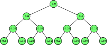
(a) Dyadic decomposition of the domain showing internal node weights.

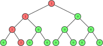
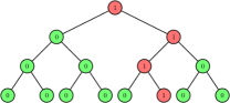
(b) Local views for two users $i$ and $j$ ($z_{i}=1$ and $z_{j}=5$) with corresponding root to leaf paths marked.

Figure 2. An example for dyadic decomposition ($B=2$)

4.2. Flat Solutions

One can observe that for an interval $[a,b]$, $R_{[a,b]}=\sum_{i=a}^{b}f_{i}$, where $f_{i}$ is the (fractional) frequency of the item $i\in[D]$. Therefore a first approach is to simply sum up estimated frequencies for every item in the range, where estimates are provided by an $\epsilon$-LDP frequency oracle: $\widehat{R}_{[a,b]}=\sum_{i=a}^{b}\widehat{\theta}_{i}$. We denote this approach (instantiated by a choice of frequency oracle $F$) as flat algorithms.

Fact 1.

For any range query $R$ of length $r$ answered using a flat method with frequency oracle $F$, $\mathrm{Var}[\widehat{R}-R]=rV_{F}$

Note that the variance grows linearly with the interval size which can be as large as $DV_{F}$.

Lemma 4.2.

The average worst case squared error over evaluation of ${D\choose 2}$ queries $\mathcal{E}$ is $\frac{1}{3}(D+2)V_{F}.$

Proof.

There are $D-r+1$ queries of length $r$. Hence the average error is $\mathcal{E}={\sum_{r=1}^{D}r(D-r+1)V_{F}}\big{/}{{D\choose 2}}=\frac{1}{3}(D+2)V_{F}$ ∎

4.3. Hierarchical Solutions

We can view the problem of answering range queries in terms of representing the frequency distribution via some collection of histograms, and producing the estimate by combining information from bins in the histograms. The “flat” approach instantiates this, and keeps one bin for each individual element. This is necessary in order to answer range queries of length 1 (i.e. point queries). However, as observed above, if we have access only to point queries, then the error grows in proportion to the length of the range. It is therefore natural to keep additional bins over subranges of the data. A classical approach is to impose a hierarchy on the domain items in such a way that the frequency of each item contributes to multiple bins of varying granularity. With such structure in place, we can answer a given query by adding counts from a relatively small number of bins. There are many hierarchical methods possible to compute histograms. Several of these have been tried in the context of centralized DP. But to the best of our knowledge, the methods that work best in centralized DP tend to rely on a complete view on the distribution, or would require multiple interactions between users and aggregator when translated to the local model. This motivates us to choose more simple yet effective strategies for histogram construction in the LDP setting. We start with the standard notion of $B$-adic intervals and a useful property of $B$-adic decompositions.

Fact 2.

For $j\in[\log_{B}D]$ and $B\in\mathbb{N}^{+}$, an interval is B-adic if it is of the form $kB^{j}...(k+1)B^{j}-1$ i.e. its length is of a power of $B$ and starts with an integer multiple of its length.

Fact 3.

Any sub-range of length $[a,b]$ of length $r$ from $[D]$ can be decomposed into $\leq(B-1)(2\log_{B}r+1)$ disjoint $B$-adic ranges.

For example, for $D=32,B=2$, the interval $[2,22]$ can be decomposed into sub-intervals $[2,3]\cup[4,7]\cup[8,15]\cup[16,19]\cup[20,21]\cup[22,22]$.

The $B$-adic decomposition can be understood as organizing the domain under a complete $B$-ary tree where each node corresponds to a bin of a unique $B$-adic range. The root holds the entire range and the leaves hold the counts for unit sized intervals. A range query can be answered by a walk over the tree similar to the standard pre-order traversal and therefore a range query can be answered with at most $2(B-1)(1+\log_{B}r)$ nodes, and at most $2(B-1)(\log_{B}D+\frac{1}{2})-1$ in the worst case.

4.4. Hierarchical Histograms (HH)

Now we describe our framework for computing hierarchical histograms. All algorithms follow a similar structure but differ on the perturbation primitive $F$ they use:

Input transformation: user $i$ locally arranges the input $z_{i}\in[D]$ in the form of a full $B$-ary tree of height $h$. Then $z_{i}$ defines a unique path from a leaf to the root with a weight of 1 attached to each node on the path, and zero elsewhere. Figure 2 shows an example. Figure 2(a) shows the dyadic ($B=2$) decomposition of the input vector $[0.1,0.15,0.23,0.12,0.2,0.05,0.07,0.08]$, where the weights on internal nodes are the sum of the weights in their subtree. Figure 2(b) illustrates two user’s local views ($z_{i}=1$ and $z_{j}=5$). In each local histogram, the nodes in the path from leaf to the root are shaded in red and have a weight of 1 on each node.

Perturbation: $i$ samples a level $l\in[h]$ with probability $p_{l}$. There are $2^{l}$ nodes at this level, with exactly one node of weight one and the rest zero. Hence, we can apply one of the mechanisms from Section 3. User $i$ perturbs this vector using some frequency oracle $F$ and sends the perturbed information to the aggregator along with the level id $l$.

Aggregation: The aggregator builds an empty tree with the same dimensions and adds the (unbiased) contribution from each user to the corresponding nodes, to estimate the fraction of the input at each node. Range queries are answered by aggregating the nodes from the $B$-adic decomposition of the range.

Key difference from the centralized case: Hierarchical histograms have been proposed and evaluated in the centralized case. However, the key difference here comes from how we generate information about each level. In the centralized case, the norm is to split the “error budget” $\epsilon$ into $h$ pieces, and report the count of users in each node; in contrast, we have each user sample a single level, and the aggregator estimates the fraction of users in each node. The reason for sampling instead of splitting emerges from the analysis: splitting would lead to an error proportional to $h^{2}$, whereas sampling gives an error which is at most proportional to $h$. Because sampling introduces some variation into the number of users reporting at each level, we work in terms of fractions rather than counts; this is important for the subsequent post-processing step.

In summary, the approach of hierarchical decomposition extends to LDP by observing the fact that it is a linear transformation of the original input domain. This means that adding information from the hierarchical decomposition of each individual’s input yields the decomposition of the entire population. Next we evaluate the error in estimation using the hierarchical methods.

Error behavior for Hierarchical Histograms. We begin by showing that the overall variance can be expressed in terms of the variance of the frequency oracle used, $V_{F}$. In what follows, we denote hierarchical histograms aggregated with fanout B as $\text{HH}_{B}$.

Theorem 4.3.

When answering a range query of length $r$ using a primitive $F$, the worst case variance $V_{r}$ under the $\text{HH}_{B}$ framework is ${V}_{r}\leq V_{F}\sum_{l=1}^{\alpha}(2B-1)\frac{1}{p_{l}}$ where $\alpha=(\lceil\log_{B}r\rceil+1)$.

Proof.

Recall that all the methods we consider have the same (asymptotic) variance bound $V_{F}=O\big{(}\frac{e^{\epsilon}}{N(e^{\epsilon}-1)^{2}}\big{)}$, with $N$ denoting the number of users contributing to the mechanism. Importantly, this does not depend on the domain size $D$, and so we can write $V_{F}\leq\psi_{F}(\epsilon)/N$, where $\psi_{F}(\epsilon)$ is a constant for method $F$ that depends on $\epsilon$. This means that once we fix the method $F$, the variance $V_{l}$ for any node at level $l$ will be the same, and is determined by $N_{l}$, the number of users reporting on level $l$. The range query $R_{[a,b]}$ of length $r$ is decomposed into at $2(B-1)$ nodes at each level, for $\alpha=\lceil\log_{B}r\rceil+1$ levels (from leaves upwards). So we can bound the total variance $\mathcal{V}^{r}$ in our estimate by

$$\sum_{l=1}^{\alpha}(2B-1)V_{l}=\sum_{l=1}^{\alpha}(2B-1)V_{F}/p_{l}=(2B-1)V_{F}\sum_{l=1}^{\alpha}\frac{1}{p_{l}}$$

using the fact that (in expectation) $N_{l}=p_{l}N$. ∎

In the worst case, $\alpha=h$, and we can minimize this bound by a uniform level sampling procedure:

Lemma 4.4.

The quantity $\sum_{l=1}^{h}\frac{1}{p_{l}}$ subject to $0\leq p_{l}\leq 1$ and $\sum_{l=1}^{h}p_{l}=1$ is minimized by setting $p_{l}=\frac{1}{h}$.

Proof.

We use the Lagrange multiplier technique, and define a new function $\mathcal{L}$, introducing a new variable $\lambda$.

$$\textstyle\mathcal{L}(p_{1},..,p_{h},\lambda)=(\sum_{l=1}^{h}\frac{1}{p_{l}})+\lambda(\sum_{l=1}^{h}p_{l}-1)$$

We compute the gradient as

$$\begin{array}[]{rl}\textstyle\nabla_{p_{1},..,p_{h},\lambda}\mathcal{L}(p_{1},..,p_{h},\lambda)&=\Big{(}\frac{\partial\mathcal{L}}{\partial p_{1}},\frac{\partial\mathcal{L}}{\partial p_{2}},..,\frac{\partial\mathcal{L}}{\partial p_{h}},\frac{\partial\mathcal{L}}{\partial\lambda}\Big{)}\\ &=\Big{(}\lambda-\frac{1}{p^{2}_{1}},..,\lambda-\frac{1}{p^{2}_{h}},\sum_{l=1}^{h}\frac{1}{p_{l}}-1\Big{)}\end{array}$$

Equating $\nabla_{p_{1},..,p_{h},\lambda}\mathcal{L}(p_{1},..,p_{h},\lambda)=0$, we get $\lambda=\frac{1}{p^{2}_{1}}=\frac{1}{p^{2}_{2}}=...=\frac{1}{p^{2}_{h}}$ and $\sum_{l=1}^{h}\frac{1}{p_{l}}=1$. Hence, $p_{l}=1/\sqrt{\lambda}=1/h$. ∎

Then, setting $p_{l}=\frac{1}{h}$ in Theorem 4.3 gives

(1) $$V_{r}\leq(2B-1)V_{F}h(\lceil\log_{B}r\rceil+1).$$

Hierarchical versus flat methods. The benefit of the HH approach over the baseline flat method depends on the factor $(2B-1)h\alpha$ versus the quantity $r$. Note that $h=\log_{B}D+O(1)$ and $\alpha=\log_{B}r+O(1)$, so we obtain an improvement over flat methods when $r>2B\log^{2}_{B}D$, for example. When $D$ is very small, this may not be achieved: for $D=64$ and $B=2$, this condition yields $r>128>D$. However, for larger $D$, say $D=2^{16}$ and $B=2$, we obtain $r>1024$, which corresponds to approximately 1.5% of the range.

Theorem 4.5.

The worst case average (squared) error incurred while answering all ${D\choose 2}$ range queries using HH_B, $\mathcal{E}_{B}$, is (approximately) $2(B-1)V_{F}\log_{B}D\log_{B}\Big{(}\frac{3D^{2}}{1+2D}\Big{)}$

Proof.

We obtain the bound by summing over all range lengths $r$. For a given length $r$, there are $D-r+1$ possible ranges. Hence,

$$\mathcal{E}_{B} \leq\frac{\sum_{r=1}^{D}V_{r}(D-r+1)}{D(D-1)/2}$$

$$=\frac{(2(B-1)V_{F}\log_{B}D)\sum_{r=1}^{D}\log_{B}r(D-r+1)}{D(D-1)/2}$$

$$=\frac{2(B-1)V_{F}\log_{B}D\Big{[}(D+1)\log_{B}(\prod_{r=1}^{D}r)-\sum_{r=1}^{D}\log_{B}r^{r}\Big{]}}{D(D-1)/2}$$

We find bounds on each of the two components separately.

1. Using Stirling’s approximation we have
$\log_{B}D!\leq\log_{B}(D^{(D+\frac{1}{2})}e^{1-D})<(D+1)\log_{B}D$.

2. Writing $P=\sum_{r=1}^{D}r=D(D+1)/2$ and $Q=\sum_{r=1}^{D}r^{2}=D(D+1)(2D+1)/6$, we make use of Jensen’s inequality to get

$$\sum_{r=1}^{D}r\log_{B}r =P\sum_{r=1}^{D}\frac{r}{P}\log_{B}r\leq P\log_{B}(\sum_{r=1}^{D}r\frac{r}{P})$$

$$=P\log_{B}(Q/P)=D(D+1)/2\log_{B}\Big{(}1+2D/3\Big{)}$$

Plugging these upper bounds in to the main expression,

$$\mathcal{E}_{B} \textstyle<\frac{2(B-1)V_{F}\log_{B}D\Big{[}(D+1)^{2}\log_{B}D-\frac{D(D+1)}{2}\log_{B}\Big{(}\frac{1+2D}{3}\Big{)}\Big{]}}{D(D-1)/2}$$

$$=\textstyle 2(B-1)V_{F}\log_{B}D\Big{[}\frac{2(D+1)^{2}\log_{B}D}{D(D-1)}-\frac{D+1}{D-1}\log_{B}\Big{(}\frac{1+2D}{3}\Big{)}\Big{]}$$

$$\approx 2(B-1)V_{F}\log_{B}D\log_{B}\Big{(}\frac{3D^{2}}{1+2D}\Big{)}\text{as }D\to\infty.$$

∎

Key difference from the centralized case: Similar looking bounds are known in centralized case, for example due to Qardaji et al. (Qardaji et al., 2013a), but with some key differences. There, the bound (simplified) is proportional to $(B-1)h^{3}V_{F}$ rather than the $(B-1)h^{2}V_{F}$ we see here. Note however that in the centralized case $V_{F}$ scales proportionate to $1/N^{2}$ rather than $1/N$ in the local case: a necessary cost to provide local privacy guarantees.

Optimal branching factor for HH_B. In general, increasing the fan-out has two consequences under our algorithmic framework. Large $B$ reduces the tree height, which increases accuracy of estimation per node since larger population is allocated to each level. But this also means that we can require more nodes at each level to evaluate a query which tends to increase the total error incurred during evaluation. We would like to find a branching factor that balances these two effects. We use the expression for the variance in (1) to find the optimal branching factor for a given $D$. We first compute the gradient of the function $2(B-1)\log_{B}(r)\log_{B}(D)$. Differentiating w.r.t. $B$ we get

$$\begin{array}[]{rl}\nabla&=\frac{D}{dB}\Big{[}\frac{2(B-1)\ln(D)\ln(r)}{\ln^{2}B}\Big{]}=2\ln D\ln r\frac{D}{dB}\Big{[}\frac{B-1}{\ln^{2}B}\Big{]}\\ &=\frac{2\ln(D)\ln(r)}{(\ln^{2}B)^{2}}\big{(}\ln^{2}B\frac{D}{dB}[B-1]-(B-1)\frac{D}{dB}[\ln^{2}B]\big{)}\\ &=2\ln D\ln r\big{(}\ln^{2}B-\frac{2}{B}(B-1)\ln B\big{)}/\ln^{4}B\\ &=2\ln D\ln r(B\ln B-2B+2)/B\ln^{3}B\end{array}$$

We now seek a $B$ such that the derivative $\nabla=0$. The numerical solution is (approximately) $B=4.922$. Hence we minimize the variance by choosing $B$ to be 4 or 5. This is again in contrast to the centralized case, where the optimal branching factor is determined to be approximately $16$ (Qardaji et al., 2013a).

4.5. Post-processing for consistency

There is some redundancy in the information materialized by the HH approach: we obtain estimates for the weight of each internal node, as well as its child nodes, which should sum to the parent weight. Hence, the accuracy of the HH framework can be further improved by finding the least squares solution for the weight of each node taking into account all the information we have about it, i.e. for each node $v$, we approximate the (fractional) frequency $f(v)$ with $\widehat{f}(v)$ such that $||f(v)-\widehat{f}(v)||_{2}$ is minimized subject to the consistency constraints. We can invoke the Gauss-Markov theorem since the variance of all our estimates are equal, and hence the least squares solution is the best linear unbiased estimator.

Lemma 4.6.

The least-squares estimated counts reduce the associated variance by a factor of at least $\frac{B}{B+1}$ in a hierarchy of fan-out $B$.

Proof.

We begin by considering the linear algebraic formulation. Let $H$ denote the $n\times D$ matrix that encodes the hierarchy, where $n$ is the number of nodes in the tree structure. For instance, if we consider a single level tree with $B$ leaves, then $H=\left[\begin{array}[]{c}\mathbf{1}_{D}\\ I_{D}\end{array}\right]$, where $\mathbf{1}_{D}$ is the $D$-length vector of all 1s, and $I_{D}$ is the $D\times D$ identity matrix. Let $\mathbf{x}$ denote the vector of reconstructed (noisy) frequencies of nodes. Then the optimal least-squares estimate of the true counts can be written as $\widehat{\mathbf{c}}=(H^{T}H)^{-1}H^{T}\mathbf{x}$. Denote a range query $R_{[a,b]}$ as the length $D$ vector that is 1 for indices between $a$ and $b$, and 0 otherwise. Then the answer to our range query is $R_{[a,b]}^{T}\widehat{\mathbf{f}}$. The variance associated with query $R_{[a,b]}$ can be found as

$$\mathrm{Var}[R_{[a,b]}^{T}\widehat{\mathbf{c}}] =\mathrm{Var}[R_{[a,b]}^{T}(H^{T}H)^{-1}H^{T}\mathbf{x}]$$

$$=R_{[a,b]}^{T}(H^{T}H)^{-1}H^{T}\mathrm{Cov}(\mathbf{x})H((H^{T}H)^{-1})^{T}R_{[a,b]}$$

$$=R_{[a,b]}^{T}(H^{T}H)^{-1}H^{T}V_{F}I_{D}H((H^{T}H)^{-1})^{T})R_{[a,b]}$$

$$=V_{F}R_{[a,b]}^{T}(H^{T}H)^{-1}(H^{T}H)((H^{T}H)^{-1})^{T})R_{[a,b]}$$

$$=V_{F}R_{[a,b]}^{T}(H^{T}H)^{-1}R_{[a,b]}$$

First, consider the simple case when $H$ is a single level tree with $B$ leaves. Then we have $H^{T}H=\mathbf{1}_{B\times B}+I_{B}$, where $\mathbf{1}_{B\times B}$ denotes the $B\times B$ matrix of all ones. We can verify that $(H^{T}H)^{-1}=((B+1)I_{B}-\mathbf{1}_{B\times B})/(B+1)$. From this we can quickly read off the variance of any range query. For a point query, the associated variance is simply $B/(B+1)V_{F}$, while for a query of length $r$, the variance is $(rB-r(r-1))/(B+1)V_{F}$. Observe that the variance for the whole range $r=B$ is just $B/(B+1)V_{F}$, and that the maximum variance is for a range of just under half the length, $r=(B+1)/2$, which gives a bound of

$V_{F}(B+1)(B+1)/(4(B+1))=(B+1)V_{F}/4$.

The same approach can be used for hierarchies with more than one level. However, while there is considerable structure to be studied here, there is no simple closed form, and forming $(H^{T}H)^{-1}$ can be inconvenient for large $D$. Instead, for each level, we can apply the argument above between the noisy counts for any node and its $B$ children. This shows that if we applied this estimation procedure to just these counts, we would obtain a bound of $B/(B+1)V_{F}$ to any node (parent or child), and at most $(B+1)V_{F}/4$ for any sum of node counts. Therefore, if we find the optimal least squares estimates, their (minimal) variance can be at most this much. ∎

Consequently, after this constrained inference, the error variance at each node is at most $\frac{BV_{F}}{B+1}$. It is possible to give a tighter bound for nodes higher up in the hierarchy: the variance reduces by $\frac{B^{i}}{\sum_{j=0}^{i}B^{j}}$ for level $i$ (counting up from level 1, the leaves). This approaches $(B-1)/B$, from above; however, we adopt the simpler $B/(B+1)$ bound for clarity.

This modified variance affects the worst case error, and hence our calculation of an optimal branching factor. From the above proof, we can obtain a new bound on the worst case error of $(B+1)V_{F}/2$ for every level touched by the query (that is, $(B+1)V_{F}/4$ for the left and right fringe of the query). This equates to $(B+1)V_{F}\log_{B}(r)\log_{B}(D)/2$ total variance. Differentiating w.r.t. $B$, we find

$$\begin{array}[]{rl}\nabla&=\frac{d}{dB}\Big{[}(B+1)\log_{B}(r)\log_{B}(D)V_{F}/2\Big{]}\\ &=\ln(r)\ln(D)(B\ln B-2B-2)/B\ln^{3}B\end{array}$$

Consequently, the value that minimizes $\nabla$ is $B\approx 9.18$ — larger than without consistency. This implies a constant factor reduction in the variance in range queries from post-processing. Specifically, if we pick $B=8$ (a power of 2), then this bound on variance is

(2) $$9V_{F}\log_{2}(r)\log_{2}(D)/(2\log_{2}^{2}8)=\frac{1}{2}V_{F}\log_{2}(r)\log_{2}(D),$$

compared to $\frac{7}{4}V_{F}\log_{2}(r)\log_{2}(D)/4$ for HH₄ without consistency. We confirm this reduction in error experimentally in Section 5.

We can make use of the structure of the hierarchy to provide a simple linear-time procedure to compute optimal estimates. This approach was introduced in the centralized case by Hay et al. (Hay et al., 2010). Their efficient two-stage process can be translated to the local model.

Stage 1: Weighted Averaging: Traversing the tree bottom up, we use the weighted average of a node’s original reconstructed frequency $f(.)$ and the sum of its children’s (adjusted) weights to update the node’s reconstructed weight. For a non-leaf node $v$, its adjusted weight is a weighted combination as follows:

$$\textstyle\bar{f}(v)=\frac{B^{i}-B^{i-1}}{B^{i}-1}f(v)+\frac{B^{i-1}-1}{B^{i}-1}\sum_{u\in\text{child}(v)}\bar{f}(u)$$

Stage 2: Mean Consistency: This step makes sure that for each node, its weight is equal to the sum of its children’s values. This is done by dividing the difference between parent’s weight and children’s total weight equally among children. For a non-root node $v$,

$$\textstyle\widehat{f}(v)=\bar{f}(v)+\frac{1}{B}\Big{[}\bar{f}(p(v))-\sum_{u\in\text{child}(v)}\bar{f}(u)\Big{]}$$

where $\bar{f}(p(v))$ is the weight of $v$’s parent after weighted averaging. The values of $\widehat{f}$ achieve the minimum $L_{2}$ solution.

Finally, we note that the cost of this post-processing is relatively low for the aggregator: each of the two steps can be computed in a linear pass over the tree structure. A useful property of finding the least squares solution is that it enforces the consistency property: the final estimate for each node is equal to the sum of its children. Thus, it does not matter how we try to answer a range query (just adding up leaves, or subtracting some counts from others) — we will obtain the same result.

Key difference from the centralized case. Our post-processing is influenced by a sequence of papers in the centralized case. However, we do observe some important points of departure. First, because users sample levels, we work with the distribution of frequencies across each level, rather than counts, as the counts are not guaranteed to sum up exactly. Secondly, our analysis method allows us to give an upper bound on the variance at every level in the tree – prior work gave a mixture of upper and lower bounds on variances. This, in conjunction with our bound on covariances allows us to give a tighter bound on the variance for a range query, and to find a bound on the optimal branching factor after taking into account the post-processing, which has not been done previously.

$$\frac{1}{\sqrt{8}}\begin{pmatrix}[r]1&1&\sqrt{2}&0&2&0&0&0\\ 1&1&\sqrt{2}&0&-2&0&0&0\\ 1&1&-\sqrt{2}&0&0&2&0&0\\ 1&1&-\sqrt{2}&0&0&-2&0&0\\ 1&-1&0&\sqrt{2}&0&0&2&0\\ 1&-1&0&\sqrt{2}&0&0&-2&0\\ 1&-1&0&-\sqrt{2}&0&0&0&2\\ 1&-1&0&-\sqrt{2}&0&0&0&-2\\ \end{pmatrix}$$

Figure 3. DHT matrix for $D=8$.

4.6. Discrete Haar Transform (DHT)

The Discrete Haar Transform (DHT) provides an alternative approach to summarizing data for the purpose of answering range queries. DHT is a popular data synopsis tool that relies on a hierarchical (binary tree-based) decomposition of the data. DHT can be understood as performing recursive pairwise averaging and differencing of our data at different granularities, as opposed to the HH approach which gathers sums of values. The method imposes a full binary tree structure over the domain, where $h(v)$ is the height of node $v$, counting up from the leaves (level 0). The Haar coefficient $c_{v}$ for a node $v$ is computed as $c_{v}=\frac{C_{l}-C_{r}}{2^{h(v)/2}}$, where $C_{l},C_{r}$ are the sum of counts of all leaves in the left and right subtree of $v$. In the local case when $z_{i}$ represents a leaf of the tree, there is exactly one non-zero haar coefficient at each level $l$ with value $\pm\frac{1}{2^{l/2}}$. The DHT can also be represented as a matrix $H_{D}$ of dimension $D\times D$ (where $D$ is a power of 2) with each row $j$ encoding the Haar coefficients for item $j\in[D]$. Figure 3 shows an instance of DHT matrix for $D=8$, i.e. $H_{8}$. In each row, the zeroth coefficient is always $\frac{1}{\sqrt{D}}$. The subsequent $D-1$ entries give weights for each of $h=\log_{2}D$ levels. For instance, for row 0, $\{\frac{1}{\sqrt{2}},0,0,0\}$, $\{\frac{1}{2},0\}$ and $\{\frac{1}{\sqrt{8}}\}$ are the sets for coefficients for levels 1, 2 and 3. We can decode the count at any leaf node $v$ by taking the inner product of the vector of Haar coefficients with the row of $H_{D}$ corresponding to $v$. Observe that we only need $h$ coefficients to answer a point query.

Answering a range query. A similar fact holds for range queries. We can answer any range query by first summing all rows of $H_{D}$ that correspond to leaf nodes within the range, then taking the inner product of this with the coefficient vector. We can observe that for an internal node in the binary tree, if it is fully contained (or fully excluded) by the range, then it contributes zero to the sum. Hence, we only need coefficients corresponding to nodes that are cut by the range query: there are at most $2h$ of these. The main benefit of DHT comes from the fact that all coefficients are independent, and there is no redundant information. Therefore we obtain a certain amount of consistency by design: any set of Haar coefficients uniquely determines an input vector, and there is no need to apply the post-processing step described in Section 4.5.

Our algorithmic framework. For convenience, we rescale each coefficient reported by a user at a non-root node to be from $\{-1,0,1\}$, and apply the scaling factor later in the procedure. Similar to the HH approach, each user samples a level $l$ with probability $p_{l}$ and perturbs the coefficients from that level using a suitable perturbation primitive. Each user then reports her noisy coefficients along with the level. The aggregator, after accepting all reports, prepares a similar tree and applies the correction to make an unbiased estimation of each Haar coefficient. The aggregator can evaluate range queries using the (unbiased but still noisy) coefficients.

Perturbing Haar coefficients. As with hierarchical histogram methods, where each level is a sparse (one hot) vector, there are several choices for how to release information about the sampled level in the Haar tree. The only difference is that previously the non-zero entry in the level was always a 1 value; for Haar, it can be a $-1$ or a $1$. There are various straightforward ways to adapt the methods that we have already (see, for example, (Bassily and Smith, 2015; Nguyên et al., 2016; Ding et al., 2017)). We choose to adapt the Hadamard Randomized Response (HRR) method, described in Section 3.2. First, this is convenient: it immediately works for negative valued weights without any modification. But it also minimizes the communication effort for the users: they summarize their whole level with a single bit (plus the description of the level and Hadmard coefficient chosen). We have confirmed this choice empirically in calibration experiments (omitted for brevity): HRR is consistent with other choices in terms of accuracy, and so is preferred for its convenience and compactness.

Recall that the (scaled) Hadamard transform of a sparse binary vector $e_{i}$ is equivalent to selecting the $i$th row/column from the Hadamard matrix. When we transform $-e_{i}$, the Hadamard coefficients remain binary, with their signs negated. Hence we use HRR for perturbing levelwise Haar coefficients. At the root level, where there is a single coefficient, this is equivalent to 1 bit RR. The 0th coefficient can be hardcoded to $\frac{N}{\sqrt{D}}$ since it does not require perturbation. We refer to this algorithm as HaarHRR.

Error behavior for HaarHRR. As mentioned before, we answer an arbitrary query of length $r$ by taking a weighted combination of at most $2h$ coefficients. A coefficient $u$ at level $l$ contributes to the answer if and only if the leftmost and rightmost leaves of the subtree of node $u$ partially overlaps with the range. The 0th coefficient is assigned the weight $r$. Let $O^{L}_{l}$ ($O^{R}_{l}$) be the size of the overlap sets for left (right) subtree for $u$ with the range. Using reconstructed coefficients, we evaluate a query to produce answer $\widehat{R}$ as below.

$$\widehat{R}=rc_{0}+2\sum_{l=1}^{h}\Big{(}\frac{O^{L}_{l}-O^{R}_{l}}{2^{l}}\Big{)}\widehat{c}_{l}$$

where, $\widehat{c}_{l}$ is an unbiased estimation of a coefficient $c_{l}$ at level $l$. In the worst case, the absolute weight $|O^{L}_{l}-O^{R}_{l}|=2^{l}$. We can analyze the corresponding varance, $V_{r}$, as

$$\begin{array}[]{rl}V_{r}&\leq 2\sum_{l=1}^{h}\Big{(}\frac{2^{l}}{2^{l+1}}\Big{)}^{2}\mathrm{Var}[\widehat{c}_{l}]=\sum_{l=1}^{h}\frac{1}{2}\mathrm{Var}[\widehat{c}_{l}]\\ &=\frac{1}{2}\sum_{l=1}^{h}\frac{V_{F}}{p_{l}}\end{array}$$

Here, $V_{F}$ is the variance associated with the HRR frequency oracle. As in the hierarchical case, the optimal choice is to set $p_{l}=1/h$ (i.e. we sample a level uniformly), where $h=\log_{2}(D)$. Then we obtain

(3) $$\textstyle V_{r}=\frac{1}{2}\log^{2}_{2}(D)V_{F}$$

It is instructive to compare this expression with the bounds obtained for the hierarchical methods. Recall that, after post-processing for consistency, we found that the variance for answering range queries with HH₈, based on optimizing the branching factor, is $\log_{2}(r)\log_{2}(D)V_{F}/2$ (from (2)). That is, for long range queries where $r$ is close to $D$, these (3) will be close to (2). Consequently, we expect both methods to be competitive, and will use empirical comparison to investigate their behavior in practice.

Finally, observe that since this bound does not depend on the range size itself, the average error across all possible range queries is also bounded by (3).

Key difference from the centralized case. The technique of perturbing Haar coefficients to answer differentially private range queries was proposed and studied in the centralized case under the name “privelets” (Xiao et al., 2011). Subsequent work argued that more involved centralized algorithms could obtain better accuracy. We will see in the experimental section that HaarHRR is among our best performing methods. Hence, our contribution in this work is to reintroduce the DHT as a useful tool in local privacy.

4.7. Prefix and Quantile Queries

Prefix queries form an important class of range queries, where the start of the range is fixed to be the first point in the domain. The methods we have developed allow prefix queries to be answered as a special case. Note that for hierarchical and DHT-based methods, we expect the error to be lower than for arbitrary range queries. Considering the error in hierarchical methods (Theorem 4.3), we require at most $B-1$ nodes at each level to construct a prefix query, instead of $(2B-1)$, which reduces the variance by almost half. For DHT similarly, we only split nodes on the right end of a prefix query, so we also reduce the variance bound by a factor of 2. Note that a reduction in variance by 0.5 will translate into a factor of $\sqrt{2}=0.707$ in the absolute error. Although the variance bound changes by a constant factor, we obtain the same optimal choice for the branching factor in $B$.

Prefix queries are sufficient to answer quantile queries. The $\phi$-quantile is that index $j$ in the domain such that at most a $\phi$-fraction of the input data lies below $j$, and at most a $(1-\phi)$ fraction lies above it. If we can pose arbitrary prefix queries, then we can binary search for a prefix $j$ such that the prefix query on $j$ meets the $\phi$-quantile condition. Errors arise when the noise in answering prefix queries causes us to select a $j$ that is either too large or too small. The quantiles then describe the input data distribution in a general purpose, non-parametric fashion. Our expectation is that our proposed methods should allow more accurate reconstructions of quantiles than flat methods, since we expect they will observe lower error. We formalize the problem:

Definition 4.7.

(Quantile Query Release Problem) Given a set of $N$ users, the goal is to collect information guaranteeing $\epsilon$-LDP to approximate any quantile $q\in[0,1]$. Let $\widehat{Q}$ be the item returned as the answer to the quantile query $q$ using a mechanism $F$, which is in truth the $q^{\prime}$ quantile, and let $Q$ be the true $q$ quantile. We evaluate the quality of $F$ by both the value error, measured by the squared error $(\widehat{Q}-Q)^{2}$; and the quantile error $|q-\widehat{q}|$.

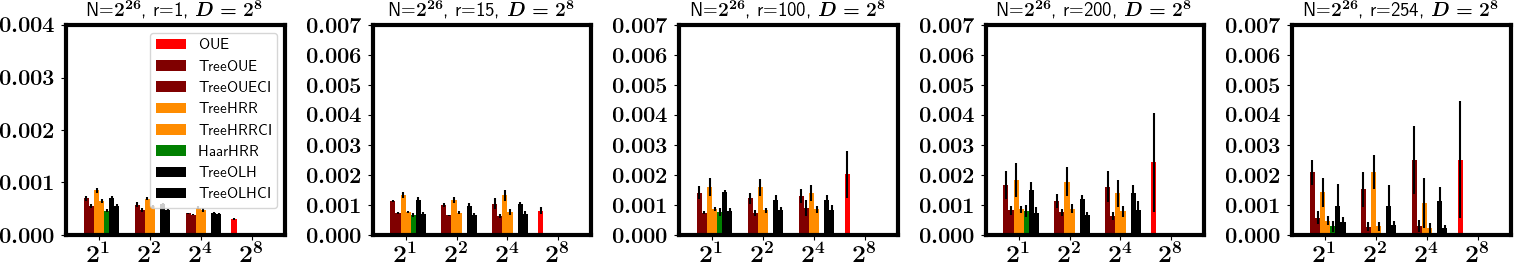
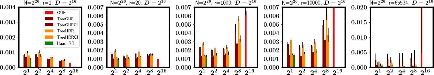
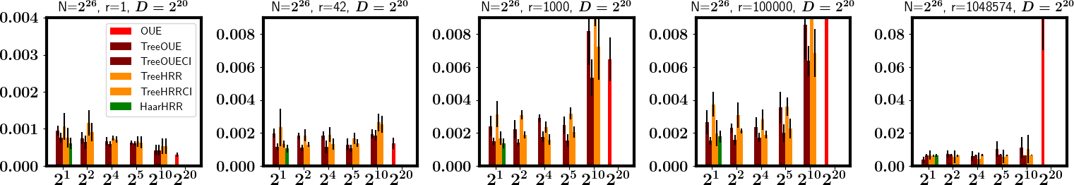
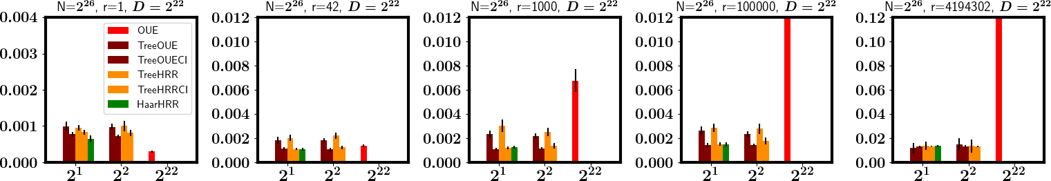
Figure 4. Impact of constrained inference and branching factor $B$. In each plot, $B$ increases along the $X$ axis, and the $Y$ axis plots the mean squared error incurred in answering all range queries of length $r$.

5. Experimental Evaluation

Our goal in this section is to validate our solutions and theoretical claims with experiments.

Dataset Used. We are interested in comparing the flat, hierarchical and wavelet methods for range queries of varying lengths on large domains, capturing meaningful real-world settings. We have evaluated the methods over a variety of real and synthetic data. Our observation is that measures such as speed and accuracy do not depend too heavily on the data distribution. Hence, we present here results on synthetic data sampled from Cauchy distributions. This allows us to easily vary parameters such as the population size $N$ and the domain size $D$, as well as varying the distribution to be more or less skewed.

The shape of the (symmetrical) Cauchy distribution is controlled by two parameters, center and height. We set the location of the center at $P\times D$, for $0<P<1$, so that larger values of $P$ shift the mass further to the right. Since Cauchy distribution has infinite support, we drop any values that fall outside $[D]$. Larger height parameters tend to reduce the sparsity in the distribution by flattening it. Our default choice is a relatively spread out distribution with height = $\frac{D}{10}$ and $P=0.4$. We vary the domain size $D$ from small ($D=2^{8}$) to large ($D=2^{22}$) as powers of two.

Algorithm default parameters and settings. We set a default value of $e^{\epsilon}=3$ ($\epsilon=1.1$), in line with prior work on LDP. This means, for example, that binary randomized response will report a true answer $\frac{3}{4}$ of the time, and lie $\frac{1}{4}$ of the time — enough to offer plausible deniability to users, while allowing algorithms to achieve good accuracy. Since the domain size $D$ is chosen to be a power of 2, we can choose a range of branching factors $B$ for hierarchical histograms so that $\log_{B}(D)$ remains an integer. The default population size $N$ is set to be $N=2^{26}$ which captures the scenario of an industrial deployment, similar to (Erlingsson et al., 2014; Pihur et al., 2018; Differential Privacy Team, Apple, 2017). Each bar plot is the mean of 5 repetitions of an experiment and error bars capture the observed standard deviation. The simulations are implemented in C++ and tested on a standard Linux machine. To the best of our knowledge, ours is among the first non-industrial work to provide simulations with domain sizes as large as $2^{22}$. Our final implementation will shortly be made available as open source.

Sampling range queries for evaluation. When the domain size is small or moderate ($D=2^{8}$ and $2^{16}$), it is feasible to evaluate all ${D\choose 2}$ range queries and so compute the exact average. However, this is not scalable for larger domains, and so we average over a subset of the range queries. To ensure good coverage of different ranges, we pick a set of evenly-spaced starting points, and then evaluate all ranges that begin at each of these points. For $D=2^{20}$ and $2^{22}$ we pick start points every $2^{15}$ and $2^{16}$ steps, respectively, yielding a total of 17M and 69M unique queries.

Histogram estimation primitives. The HH framework in general is agnostic to the choice of the histogram estimation primitive $F$. We show results with OUE, HRR and OLH as the primitives for histogram reconstruction, since they are considered to be state of art (Wang et al., 2017), and all provide the same theoretical bound $V_{F}$ on variance. Though any of these three methods can serve as a flat method, we choose OUE as a flat method since it can be simulated efficiently and reliably provides the lowest error in practice by a small margin. We refer to the hierarchical methods using HH framework as TreeOUE, TreeOLH and TreeHRR. Their counterparts where the aggregator applies postprocessing to enforce consistency are identified with the CI suffix, e.g. TreeHRRCI.

We quickly observed in our preliminary experiments that direct implementation of OUE can be very slow for large $D$: the method perturbs and reports $D$ bits for each user. For accuracy evaluation purposes, we can replace the slow method with a statistically equivalent simulation. That is, we can simulate the aggregated noisy count data that the aggregator would receive from the population. We know that noisy count of any item is aggregated from two distributions (1) “true” ones that are reported as ones (with prob. $\frac{1}{2}$) (2) zeros that are flipped to be ones (with prob. $\frac{1}{1+e^{\epsilon}}$). Therefore, using the (private) knowledge of the true count $\theta[j]$ of item $j\in[D]$, the noisy count $\theta^{*}[j]$ can be expressed as a sum of two binomial random variables, $\theta^{*}[j]=\text{Bino}(\theta[j],0.5)+\text{Bino}\Big{(}N-\theta[j],\frac{1}{1+e^{\epsilon}}\Big{)}.$ Our simulation can perform this sampling for all items, then provides the sampled count to the aggregator, which then performs the usual bias correction procedure.

The OLH method suffers from a more substantial drawback: the method is very slow for the aggregator to decode, due to the need to iterate through all possible inputs for each user report (time $O(ND)$). We know of no short cuts here, and so we only consider OLH for our initial experiments with small domain size $D$.

$\epsilon$	HH${}^{c}_{2}$	HH${}^{c}_{4}$	HH${}^{c}_{16}$	HaarHRR
0.2	4.269	4.037	4.176	3.684
0.4	2.024	2.193	2.590	1.831
0.6	1.388	1.341	1.535	1.278
0.8	1.002	0.950	1.130	0.987
1.0	0.844	0.744	0.844	0.811
1.1	0.722	0.667	0.820	0.748
1.2	0.684	0.658	0.642	0.732
1.4	0.571	0.542	0.592	0.601

(a) $D=2^{8}$

$\epsilon$	HH${}^{c}_{2}$	HH${}^{c}_{4}$	HH${}^{c}_{16}$	HaarHRR
0.2	6.745	7.129	8.692	6.666
0.4	3.616	3.424	4.648	3.526
0.6	2.333	2.360	2.793	2.342
0.8	1.644	1.728	2.075	1.711
1.0	1.356	1.377	1.642	1.484
1.1	1.303	1.270	1.597	1.345
1.2	1.090	1.140	1.433	1.201
1.4	0.922	0.995	1.158	1.130

(b) $D=2^{16}$

$\epsilon$	HH${}^{c}_{2}$	HH${}^{c}_{4}$	HH${}^{c}_{16}$	HaarHRR
0.2	10.043	10.493	11.511	9.285
0.4	5.378	4.751	5.617	5.261
0.6	3.605	3.603	4.483	3.693
0.8	3.047	3.042	3.352	3.316
1.0	2.522	2.690	3.131	2.915
1.1	2.556	2.540	2.729	2.722
1.2	2.619	2.488	2.757	2.640
1.4	2.339	2.304	2.652	2.505

(c) $D=2^{20}$

$\epsilon$	HH${}^{c}_{2}$	HH${}^{c}_{4}$	HaarHRR
0.2	8.629	8.889	8.422
0.4	4.546	4.951	4.470
0.6	3.181	3.420	3.085
0.8	2.657	2.692	2.462
1.0	2.247	2.358	2.254
1.1	1.979	2.252	2.139
1.2	2.120	2.066	1.946
1.4	1.650	1.885	1.990

(d) $D=2^{22}$

Figure 5. Impact of varying $\epsilon$ on mean squared error for arbitrary queries. These numbers are scaled up by 1000 for presentation.

$\epsilon$	HH${}^{c}_{2}$	HH${}^{c}_{4}$	HH${}^{c}_{16}$	HaarHRR
0.2	4.306	2.968	4.282	2.857
0.4	1.859	1.439	1.828	1.377
0.6	1.366	0.957	1.758	1.031
0.8	0.937	0.778	0.896	0.758
1.0	0.802	0.561	0.637	0.613
1.1	0.684	0.533	0.666	0.626
1.2	0.658	0.437	0.670	0.568
1.4	0.573	0.420	0.478	0.494

(a) $D=2^{8}$

$\epsilon$	HH${}^{c}_{2}$	HH${}^{c}_{4}$	HH${}^{c}_{16}$	HaarHRR
0.2	7.701	6.172	7.014	5.870
0.4	3.266	3.101	3.744	2.880
0.6	2.402	2.176	2.426	2.018
0.8	1.663	1.503	1.834	1.511
1.0	1.338	1.220	1.426	1.244
1.1	1.202	1.051	1.259	1.120
1.2	1.080	0.978	1.147	1.054
1.4	0.973	0.848	0.981	0.973

(b) $D=2^{16}$

$\epsilon$	HH${}^{c}_{2}$	HH${}^{c}_{4}$	HH${}^{c}_{16}$	HaarHRR
0.2	8.874	8.255	10.462	7.237
0.4	4.734	4.395	5.754	4.271
0.6	3.788	3.485	4.055	3.377
0.8	3.287	3.094	3.268	3.108
1.0	3.022	2.848	2.826	2.920
1.1	3.053	2.756	2.727	2.727
1.2	3.145	2.627	2.914	2.754
1.4	2.975	2.659	2.543	2.696

(c) $D=2^{20}$

$\epsilon$	HH${}^{c}_{2}$	HH${}^{c}_{4}$	HaarHRR
0.2	8.620	8.638	8.099
0.4	4.181	4.330	4.233
0.6	2.932	3.077	3.063
0.8	2.215	2.590	2.528
1.0	1.958	2.246	2.326
1.1	1.777	2.319	2.181
1.2	1.929	2.174	2.205
1.4	1.613	1.868	2.156

(d) $D=2^{22}$

Figure 6. Impact of varying $\epsilon$ on mean squared for prefix queries. These numbers are scaled up by 1000 for presentation. We underline the scores that are smaller than corresponding scores in Figure 6.

D	$2^{8}$	$2^{9}$	$2^{10}$	$2^{11}$
Wavelet	221.62	306.31	410.29	536.32
(optimal) HH${}^{c}_{16}$	79.23	164.48	185.94	213.87
HH${}^{c}_{2}$	220.06	305.54	409.48	535.63
$\frac{\text{Wavelet}}{\text{HH}^{c}_{16}}$	2.7971	1.8622	2.20	2.5077
$\frac{\text{HH}^{c}_{2}}{\text{HH}^{c}_{16}}$	2.777	1.8576	2.202	2.5044

Figure 7. Table 3 from (Qardaji et al., 2013a) comparing the exact average variance incurred in answering all range queries for $\epsilon=1$ in the centralized case.

5.1. Impact of varying $B$ and $r$

Experiment description. In this experiment, we aim to study how much a privately reconstructed answer for a range query deviates from the ground truth. Each query answer is normalized to fall in the range 0 to 1, so we expect good results to be much smaller than 1. To compare with our theoretical analysis of variance, we measure the accuracy in the form of mean squared error between true and reconstructed range query answers.

Plot description. Figure 4 illustrates the effect of branching factor $B$ on accuracy for domains of size $2^{8}$ (small), $2^{16}$ (medium), and lastly $2^{20}$ and $2^{22}$ (large). Within each plot with a fixed $D$ and query length $r$, we vary the branching factor on the $X$ axis. We plot the flat OUE method as if it were a hierarchical method with $B=D$, since it effectively has this fan out from the root. We treat HaarHRR as if it has $B=2$, since is based on a binary tree decomposition. The $Y$ axis in each plot shows the mean squared error incurred while answering all queries of length $r$. As the plots go left to right, the range length increases from 1 to just less than the whole domain size $D$. The top row of plots have $D=2^{8}$, and the last row of plots have $D=2^{22}$.

Observations. Our first observation is that the CI step reliably provides a significant improvement in accuracy in almost all cases for HH, and never increases the error. Our theory suggests that the CI step improves the worst case accuracy by a constant factor, and this is borne out in practice. This improvement is more pronounced at larger intervals and higher branching factors. In many cases, especially in the right three columns, TreeOUECI and TreeHRRCI are two to four times more accurate then their inconsistent counter parts. Consequently, we put our main focus on methods with consistency applied in what follows.

Next, we quickly see evidence that the flat approach (represented by OUE) is not effective for answering range queries. Unsurprisingly, for point queries ($r=1$), flat methods are competitive. This is because all methods need to track information on individual item frequencies, in order to answer short range queries. The flat approach keeps only this information, and so maximizes the accuracy here. Meanwhile, HH methods only use leaf level information to answer point queries, and so we see better accuracy the shallower the tree is, i.e. the bigger $B$ is. However, as soon as the range goes beyond a small fraction of the domain size, other approaches are preferable. The second column of plots shows results for relatively short ranges where the flat method is not the most accurate.

For larger domain sizes and queries, our methods outperform the flat method by a high margin. For example, the best hierarchical methods for very long queries and large domains are at least 16 times more accurate than the flat method. Recall our discussion of OLH above that emphasised that its computation cost scales poorly with domain size $D$. We show results for TreeOLH and TreeOLHCI for the small domain size $2^{8}$, but drop them for larger domain sizes, due to this poor scaling. We can observe that although the method acheives competitive accuracy, it is equalled or beaten by other more performant methods, so we are secure in omitting it.

As we consider the two tree methods, TreeOUE and TreeHRR, we observe that they have similar patterns of behavior. In terms of the branching factor $B$, it is difficult to pick a single particular $B$ to minimize the variance, due to the small relative differences. The error seems to decrease from $B=2$, and increase for larger $B$ values above $2^{4}$ (i.e. 16). Across these experiments, we observe that choosing $B=4$, 8 or 16 consistently provides the best results for medium to large sized ranges. This agrees with our theory, which led us to favor $B=8$ or $B=4$, with or without consistency applied respectively. This range of choices means that we are not penalized severely for failing to choose an optimal value of $B$.

The main takeaway from Figure 4 is the strong performance for the HaarHRR method. It is not competitive for point queries ($r=1$), but for all ranges except the shortest it achieves the single best or equal best accuracy. For some of the long range queries covering the almost the entire domain, it is slightly outperformed by consistent HH_B methods. However, this is sufficiently small that it is hard to observe visually on the plots. Across a broad range of query lengths (roughly, 0.1% to 10% of the domain size), HaarHRR is preferred. It is most clearly the preferred method for smaller domain sizes, such as in the case of $D=2^{8}$. We observed a similar behavior for domains as small as $2^{5}$.

5.2. Impact of privacy parameter $\epsilon$

Experiment description. We now vary $\epsilon$ between 0.1 (higher privacy) to 1.4 (lower privacy) and find the mean squared error over range queries. Similar ranges of $\epsilon$ parameters are used in prior works such as (Zhang et al., 2018). After the initial exploration documented in the previous section, our goal now is to focus in on the most accurate and scalable hierarchical methods. Therefore, we omit all flat methods and consider only those values of $B$ that provided satisfactory accuracy. We choose TreeOUECI as our mechanism to instantiate HH (henceforth denoted by HH${}^{c}_{B}$, where the $c$ denotes that consistency is applied) method due to its accuracy. We do note that a deployment may prefer TreeHRRCI over TreeOUECI since it requires vastly reduced communication for each user at the cost of only a slight increase in error.

Plot description. Table 6 compares the mean squared error for HH${}^{c}_{2}$, HH${}^{c}_{4}$ HH${}^{c}_{16}$ and HaarHRR for various $\epsilon$ values. We multiply all results by a factor of 1000 for convenience, so the typical values are around $10^{-3}$ corresponding to very low absolute error. In each row, we mark in bold the lowest observed variance, noting that in many cases, the “runner-up” is very close behind.

Observations. The first observation, consistent with Figure 4, is that for lower $\epsilon$’s, HaarHRR is more accurate than the best of HH${}^{c}_{B}$ methods. This improvement is most pronounced for $D=2^{8}$ i.e. at most 10% (at $\epsilon=0.2$) and marginal (0.01 to 1%) for larger domains. For larger $\epsilon$ regimes, HH${}^{c}_{B}$ outperforms HaarHRR, but only by a small margin of at most 11%. For large domains, HH${}^{c}_{B}$ remains the best method. In general, except for $D=2^{22}$, there is no one value of $B$ that achieves the best results at all parameters but overall $B=4$ yields slightly more accurate results for HH${}^{c}_{B}$ for most cases. Note that this $B$ value is closer to the optimal value of 9 (derived in Section 4.5) than other values. When $D=2^{22}$, HH${}_{2}^{c}$ dominates HH${}_{4}^{c}$ but only by a margin of at most 10%.

Comparison with DHT and HH based approaches in the centralized case. We briefly contrast with the conclusion in the centralized case. We reproduce some of the results of Qardaji et al. (Qardaji et al., 2013a) in Table 7, comparing variance for the (centralized) wavelet based approach to (centralized) hierarchical histogram approaches with $B=2,16$ with consistency applied. These numbers are scaled and not normalized, so can’t be directly compared to our results (although, we know that the error should be much lower in the centralized case). However, we can meaningfully compare the ratio of variances, which we show in the last two rows of the table.

For $\epsilon=1,D=2^{8}$, the error for the Haar method is approximately $2.8$ times more than the hierarchical approach. Meanwhile, the corresponding readings for HaarHRR and HH${}^{c}_{4}$ (the most accurate method in the $\epsilon=1$ row) in Table 6 are 0.787 and 0.763 — a deviation of only $\approx$3%. Another important distinction from the centralized case is that we are not penalized a lot for choosing a sub-optimal branching factor. Whereas, we see in the 4th row that choosing $B=2$ increases the error of consistent HH method by at least 1.8576 times from the preferred method HH${}^{c}_{16}$.

A further observation is that (apart for $D=2^{22}$) across 24 observations, HaarHRR is never outperformed by all values of HH${}^{c}_{B}$ i.e. in no instance is it the least accurate method. It trails the best HH${}^{c}_{B}$ method by at most 10%. On the other hand, in the centralized case (Table 7), the variance for the wavelet based approach is at least 1.86 times higher than HH${}^{c}_{B}$.

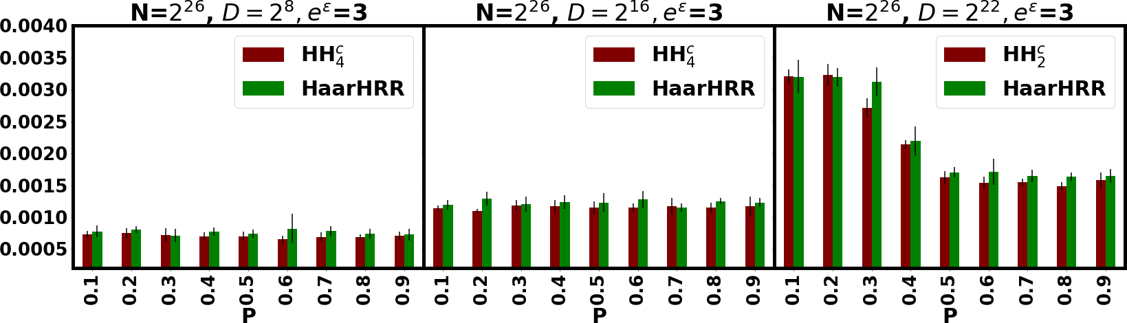
Figure 8. Impact of varying the distribution center ($P\times D$) on mean squared error for various domain sizes $D$.

5.3. Prefix Queries

Experiment description. As described in Section 4.7, prefix queries deserve special attention. Our set up is the same as for range queries. We evaluate every prefix query, as there are fewer of them.

Plot description. Table 6 is the analogue of Table 6 for prefix queries, computed with the same settings. We underline the scores that are smaller than corresponding scores in Table 6.

Observations. The first observation is that the error in Table 6 is often smaller (up to 30%) than in Table 6 at many instances, particularly for small and medium sized domains. The reduction is not as sharp as the analysis might suggest, since that only gives upper bounds on the variance. Reductions in error are not as noticeable for larger values of $D$, although this could be impacted by our range query sampling strategy. In terms of which method is preferred, HH${}^{c}_{2}$ for $D=2^{22}$ and HH${}_{4}^{c}$ tend to dominate for larger $\epsilon$, while HaarHRR is preferred for smaller $\epsilon$.

5.4. Impact of input distribution

Experiment description. We now check whether the shape of the input distribution affects the mean squared error when other parameters are held to their default values.

Plot description. Figure 8 plots the mean squared error for domains of different sizes for $e^{\epsilon}=3$ ($\epsilon=1.1$). Along the $X$ axis, we shift the center of the Cauchy distribution by changing $0<P<1$. For each domain size $D$, we make our comparison between HaarHRR and the most accurate consistent HH method according to Table 6.

Observations. The chief observation is that for small and mid sized domains, the change in distribution does not make any noticeable difference in the accuracy. HaarHRR continues to be slightly inferior to HH${}_{4}^{c}$ for all input shapes. For $D=2^{22}$, we do notice an increase in the error when the bulk of the mass of the distribution is towards the left end of the domain ($P=0.1$ to $P=0.3$). This is partly due to the range sampling method we use: the majority of range queries we test cover only a small amount of the true probability mass of the distribution for these $P$ values, and this leads to increased error from privacy noise. However, the main take-away here should be the consistently small absolute numbers: maximum mean squared error of 0.0035, i.e. very accurate answers.

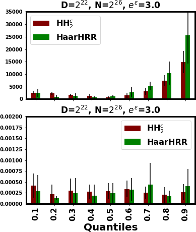
(a) $P=0.1$

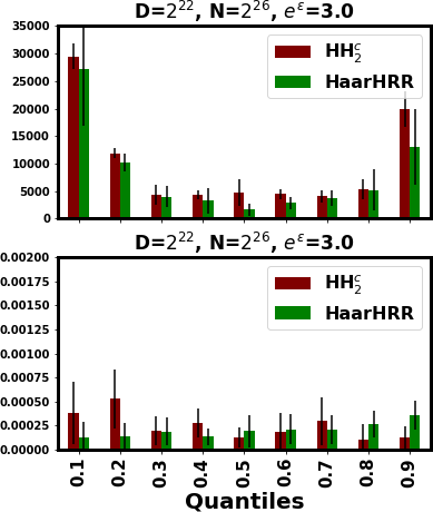
(b) $P=0.5$

Figure 9. Top row: value error; bottom row: quantile error

5.5. Quantile Queries

Experiment description. Finally, we compare the performance of the best hierarchical approaches in evaluation of the deciles (i.e. the $\phi$-quantiles for $\phi$ in 0.1 to 0.9) for a left skewed ($P=0.1$) and centered ($P=0.5$) Cauchy distribution.

Plot description. The top row in Figure 9 plots the actual difference between true and reconstructed quantile values (value error). The corresponding bottom plots measure the absolute difference between the quantile value of the returned value and the target quantile (quantile error).

Observations. The first observation is that the both the algorithms have low absolute value error (the top row). For the domain of $2^{22}\approx 4M$, even the largest error of $\approx$35K made by HH${}_{2}^{c}$ is still very small, and less than 1%. The value error tends to be highest where the data is least dense: towards the right end when the data skews left ($P=0.1$), and at either extreme when the data is centered. Importantly, the corresponding quantile error is mostly flat. This means that instead of finding the median (say), our methods return a value that corresponds to the 0.5004 quantile, which is very close in the distributional sense. This reassures us that any spikes in the value error are mostly a function of sparse data, rather than problems with the methods.

5.6. Experimental Summary

We can draw a number of conclusions and recommendations from this study:

$\bullet$ The flat methods are never competitive, except for very short ranges and small domains.

$\bullet$ The wavelet approach is preferred for small values of $\epsilon$ (roughly $\epsilon<0.8$), while the (consistent) HH approach is preferred for larger $\epsilon$’s and for larger queries.

$\bullet$ This threshold is slightly reduced for larger domains. However, the “regret” for choosing a “wrong” method is low: the difference between the best method and its competitor from HH and wavelet is typically no more than 10-%.

$\bullet$ Overall, the wavelet approach (HaarHRR) is always a good compromise method. It provides accuracy comparable to consistent HH in all settings, and requires a constant factor less space ($D$ wavelet coefficients against $2D-1$ for HH₂).

6. Concluding Remarks

We have seen that we can accurately answer range queries under the model of local differential privacy. Two methods whose counterparts have quite differing behavior in the centralized setting are very similar under the local setting, in line with our theoretical analysis. Now that we have reliable primitives for range queries and quantiles, it is natural to consider how to extend and apply them further.

Multidimensional range queries. Both the hierarchical and wavelet approaches can be extended to multiple dimensions. Consider applying the hierarchical decomposition to two-dimensional data, drawn from the domain $[D]^{2}$. Now any (rectangular) range can be decomposed into $\log_{B}^{2}D$ $B$-adic rectangles (where each side is drawn from a $B$-adic decomposition), and so we can bound the variance in terms of $\log_{B}^{4}D$. More generally, we achieve variance depending on $\log^{2d}D$ for $d$-dimensional data. Similar bounds apply for generalizations of wavelets. These give reasonable bounds for small values of $d$ (say, 2 or 3). For higher dimensions, we anticipate that coarser gridding approaches would be preferred, in line with (Qardaji et al., 2013b).

Advanced data analysis. In the abstract, many tasks in data modeling and prediction can be understood as building a description of observed data density. For example, many (binary) classification problems can be described as trying to predict what class is most prevalent in the neighborhood of a given query point. Viewed through this lens, range queries form a primitive that can be used to build such model. As a simple example, consider building a Naive Bayes classifier for a public class based on private numerical attributes. If we use our methods to allow range queries to be evaluated on each attribute for each class, we can then build models for the prediction problem. Generalizations of this approach to more complex models, different mixes of public and private attributes, and different questions, give a set of open problems for this area.

Acknowledgements. This work is supported in part by AT&T, European Research Council grant ERC-2014-CoG 647557, and The Alan Turing Institute under the EPSRC grant EP/N510129/1.

References

- (1)
- Bassily et al. (2017) Raef Bassily, Kobbi Nissim, Uri Stemmer, and Abhradeep Guha Thakurta. 2017. Practical Locally Private Heavy Hitters. In NIPS. 2285–2293.
- Bassily and Smith (2015) Raef Bassily and Adam Smith. 2015. Local, private, efficient protocols for succinct histograms. In Proceedings of ACM STOC. ACM, 127–135.
- Chang and Thakurta (2018) Johnnie C-N. Chang and Abhradeep Guha Thakurta. 2018. Autocompletion with Local Differential Privacy. In IEEE Security and Privacy Symposium.
- Cormode et al. (2012) Graham Cormode, Minos Garofalakis, Peter Haas, and Chris Jermaine. 2012. Synposes for Massive Data: Samples, Histograms, Wavelets and Sketches. NOW publishers.
- Cormode et al. (2018) Graham Cormode, Tejas Kulkarni, and Divesh Srivastava. 2018. Marginal Release Under Local Differential Privacy. In Proceedings of ACM SIGMOD. 131–146.
- Cormode et al. (2012) Graham Cormode, Cecilia M. Procopiuc, Divesh Srivastava, Entong Shen, and Ting Yu. 2012. Differentially Private Spatial Decompositions. In IEEE 28th International Conference on Data Engineering. 20–31.
- Differential Privacy Team, Apple (2017) Differential Privacy Team, Apple. 2017. Learning With Privacy At Scale. Apple Machine Learning Journal (2017). https://machinelearning.apple.com/docs/learning-with-privacy-at-scale/appledifferentialprivacysystem.pdf
- Ding et al. (2017) Bolin Ding, Janardhan Kulkarni, and Sergey Yekhanin. 2017. Collecting Telemetry Data Privately. In Advances in Neural Information Processing Systems 30. https://www.microsoft.com/en-us/research/publication/collecting-telemetry-data-privately/
- Duchi et al. (2013) John C Duchi, Michael I Jordan, and Martin J Wainwright. 2013. Local privacy and statistical minimax rates. In FOCS. IEEE.
- Dwork et al. (2006) Cynthia Dwork, Frank Mcsherry, Kobbi Nissim, and Adam Smith. 2006. Calibrating Noise to Sensitivity in Private Data Analysis. In Theory of Cryptography Conference.
- Dwork and Roth (2014) Cynthia Dwork and Aaron Roth. 2014. The Algorithmic Foundations of Differential Privacy. NOW publishers.
- Erlingsson et al. (2014) Úlfar Erlingsson, Vasyl Pihur, and Aleksandra Korolova. 2014. RAPPOR: Randomized Aggregatable Privacy-Preserving Ordinal Response. In ACM CCS. https://doi.org/10.1145/2660267.2660348
- Fanti et al. (2016) Giulia Fanti, Vasyl Pihur, and Úlfar Erlingsson. 2016. Building a RAPPOR with the unknown: Privacy-preserving learning of associations and data dictionaries. Proceedings on Privacy Enhancing Technologies 2016, 3 (2016), 41–61.
- Gao et al. (2018) Tianchong Gao, Feng Li, Yu Chen, and Xukai Zou. 2018. Local Differential Privately Anonymizing Online Social Networks Under HRG-Based Model. IEEE Trans. Comput. Social Systems 5, 4 (2018), 1009–1020. https://doi.org/10.1109/TCSS.2018.2877045
- Hardt et al. (2012) Moritz Hardt, Katrina Ligett, and Frank McSherry. 2012. A Simple and Practical Algorithm for Differentially Private Data Release. In Advances in Neural Information Processing Systems. 2348–2356.
- Hay et al. (2010) Michael Hay, Vibhor Rastogi, Gerome Miklau, and Dan Suciu. 2010. Boosting the Accuracy of Differentially Private Histograms Through Consistency. Proc. VLDB Endow. 3, 1-2 (Sept. 2010), 1021–1032. https://doi.org/10.14778/1920841.1920970
- Kairouz et al. (2016) Peter Kairouz, Keith Bonawitz, and Daniel Ramage. 2016. Discrete Distribution Estimation Under Local Privacy. In Proceedings of ICML. 2436–2444. http://dl.acm.org/citation.cfm?id=3045390.3045647
- Kasiviswanathan et al. (2011) Shiva Prasad Kasiviswanathan, Homin K. Lee, Kobbi Nissim, Sofya Raskhodnikova, and Adam D. Smith. 2011. What Can We Learn Privately? SIAM J. Comput. 40, 3 (2011), 793–826. https://doi.org/10.1137/090756090
- Nguyên et al. (2016) Thông T. Nguyên, Xiaokui Xiao, Yin Yang, Siu Cheung Hui, Hyejin Shin, and Junbum Shin. 2016. Collecting and Analyzing Data from Smart Device Users with Local Differential Privacy. CoRR abs/1606.05053 (2016). http://arxiv.org/abs/1606.05053
- Pihur et al. (2018) Vasyl Pihur, Aleksandra Korolova, Frederick Liu, Subhash Sankuratripati, Moti Yung, Dachuan Huang, and Ruogu Zeng. 2018. Differentially-Private “Draw and Discard” Machine Learning. In 4th Workshop on the Theory and Practice of Differential Privacy at CCS. https://arxiv.org/abs/1807.04369
- Qardaji et al. (2013a) Wahbeh Qardaji, Weining Yang, and Ninghui Li. 2013a. Understanding Hierarchical Methods for Differentially Private Histograms. Proc. VLDB Endow. 6, 14 (Sept. 2013), 1954–1965. https://doi.org/10.14778/2556549.2556576
- Qardaji et al. (2013b) Wahbeh H. Qardaji, Weining Yang, and Ninghui Li. 2013b. Differentially private grids for geospatial data. In Proceedings of IEEE ICDE. 757–768.
- Qin et al. (2017) Zhan Qin, Ting Yu, Yin Yang, Issa Khalil, Xiaokui Xiao, and Kui Ren. 2017. Generating Synthetic Decentralized Social Graphs with Local Differential Privacy. In CCS. ACM, 425–438.
- Samet (2005) Hanan Samet. 2005. Foundations of Multidimensional and Metric Data Structures. Morgan Kaufmann.
- Shin et al. (2018) Hyejin Shin, Sungwook Kim, Junbum Shin, and Xiaokui Xiao. 2018. Privacy Enhanced Matrix Factorization for Recommendation with Local Differential Privacy. IEEE Trans. Knowl. Data Eng. 30, 9 (2018), 1770–1782. https://doi.org/10.1109/TKDE.2018.2805356
- Wang et al. (2019) Ning Wang, Xiaokui Xiao, Yin Yang, Jun Zhao, Siu Cheung Hui, Hyejin Shin, Junbum Shin, and Ge Yu. 2019. Collecting and Analyzing Multidimensional Data with Local Differential Privacy. In Proceedings of IEEE ICDE.
- Wang et al. (2017) Tianhao Wang, Jeremiah Blocki, Ninghui Li, and Somesh Jha. 2017. Locally Differentially Private Protocols for Frequency Estimation. In Proceedings of the USENIX Security Symposium. 729–745. https://www.usenix.org/conference/usenixsecurity17/technical-sessions/presentation/wang-tianhao
- Warner (1965) S. L. Warner. 1965. Randomised response: a survey technique for eliminating evasive answer bias. J. Amer. Statist. Assoc. 60, 309 (March 1965), 63–69.
- Xiao et al. (2011) Xiaokui Xiao, Guozhang Wang, and Johannes Gehrke. 2011. Differential Privacy via Wavelet Transforms. IEEE Trans. Knowl. Data Eng. 23, 8 (2011), 1200–1214. https://doi.org/10.1109/TKDE.2010.247
- Zhang et al. (2018) Zhikun Zhang, Tianhao Wang, Ninghui Li, Shibo He, and Jiming Chen. 2018. CALM: Consistent Adaptive Local Marginal for Marginal Release under Local Differential Privacy. In Proceedings of ACM CCS 2018. 212–229.
- Zheng et al. (2017) Kai Zheng, Wenlong Mou, and Liwei Wang. 2017. Collect at Once, Use Effectively: Making Non-interactive Locally Private Learning Possible. In Proceedings of ICML. 4130–4139.