Essential elements for nuclear binding

Abstract

How does nuclear binding emerge from first principles? Our current best understanding of nuclear forces is based on a systematic low-energy expansion called chiral effective field theory. However, recent ab initio calculations of nuclear structure have found that not all chiral effective field theory interactions give accurate predictions with increasing nuclear density. In this letter we address the reason for this problem and the first steps toward a solution. Using nuclear lattice simulations, we deduce the minimal nuclear interaction that can reproduce the ground state properties of light nuclei, medium-mass nuclei, and neutron matter simultaneously with no more than a few percent error in the energies and charge radii. We find that only four parameters are needed. With these four parameters one can accurately describe neutron matter up to saturation density and the ground state properties of nuclei up to calcium. Given the absence of sign oscillations in these lattice Monte Carlo simulations and the mild scaling of computational effort scaling with nucleon number, this work provides a pathway to high-quality simulations in the future with as many as one or two hundred nucleons.

Chiral effective field theory ($\chi$EFT) is a first principles approach to nuclear forces where interactions are arranged as a low-energy expansion in powers of momentum and pion mass Epelbaum:2008ga ; Machleidt:2011zz . While many calculations establish the reliability of $\chi$EFT in describing the properties of light nuclei Hupin:2014iqa ; Navratil:2007aj ; Lonardoni:2017hgs ; Piarulli:2017dwd ; Epelbaum:2018ogq , the binding energies and charge radii of medium mass nuclei are not consistently reproduced  Wloch:2005za ; Hagen:2008iw ; Hagen:2012sh ; Binder:2013xaa ; Epelbaum:2013paa ; Cipollone:2014hfa ; Ekstrom:2015rta ; Lonardoni:2017hgs . One well-known example is that the charge radius of ¹⁶O tends to be too small for most of interactions in the literature Wloch:2005za ; Hagen:2012sh ; Binder:2013xaa ; Epelbaum:2013paa ; Cipollone:2014hfa . The core issue is that $\chi$EFT many-body calculations do not yet give reliable and accurate predictions at higher nuclear densities. We note that there have been efforts to improve the convergence of many-body calculations by rearranging the chiral effective field theory expansion at nonzero density Meissner:2001gz ; Lacour:2009ej . If one reaches high enough orders in the $\chi$EFT expansion, then the systematic errors will eventually decrease as more and more low-energy parameters are tuned to empirical data. However, the predictive power of the ab initio approach will be diminished as more data will be needed to constrain the higher-body forces. Furthermore, the computational effort will increase significantly to the point where a first principles treatment may not be practical.

One pragmatic approach is to further constrain the nuclear force using nuclear structure data from medium mass nuclei or the saturation properties of nuclear matter Ekstrom:2015rta . This approach has been applied successfully in several recent calculations Hagen:2015yea ; Hagen:2016uwj ; Simonis:2017dny ; Morris:2017vxi . A rather different line of investigation has looked at the microscopic origins of the problem. In Ref. Elhatisari:2016owd numerical evidence is shown that nuclear matter sits near a quantum phase transition between a Bose gas of alpha particles and nuclear liquid. It is argued that local SU(4)-invariant forces play an increasingly important role at higher nuclear densities. The term local refers to velocity-independent interactions, as opposed to nonlocal interactions which are velocity dependent. The SU(4) refers to Wigner’s approximate symmetry of the nuclear interactions where the four nucleonic degrees of freedom (proton spin-up, proton spin-down, neutron spin-up, neutron spin-down) can be rotated into each other Wigner:1936dx .

The importance of SU(4)-invariant interactions can be understood in terms of coherent enhancement. Spin-dependent forces tend to cancel when summing over all possible nucleonic spin configurations. For example, we have seen in lattice calculations of binding energies for closed shell systems that the contribution from the repulsive P-wave channels often cancels most of the contribution from the attractive P-wave channels. We note also the intriguing analysis in Ref. CalleCordon:2009ps which demonstrates the connection between quantum chromodynamics with a large number of colors to Wigner’s SU(4) symmetry for the S-wave interactions and Serber symmetry for the P-wave interactions. Similarly most isospin-dependent forces tend to cancel in symmetric nuclear matter due to the equal number of protons and neutrons, the one notable exception being the Coulomb interaction. The idea of SU(4) universality at large S-wave scattering length has a rich history in nuclear physics. It is well known that the Tjon line relating ³H and ⁴He binding energies is a manifestation of universality in nuclear systems Platter:2004zs ; Klein:2018lqz . It has also been shown that ³H and ⁴He are characterized by universal physics associated with the Efimov effect Konig:2016utl ; Kievsky:2015dtk . The coherent enhancement of SU(4)-invariant forces in the nuclear many-body environment suggests a possible resurgence of SU(4) symmetry in heavier nuclei as well. This idea inspired the exploratory work in Ref. Elhatisari:2017eno on the structure of nuclei up through oxygen using an SU(4)-invariant interaction. This built upon previous work in Ref. Elhatisari:2016owd which showed that local SU(4)-invariant interactions have a particularly strong effect on nuclear binding. The special role of local forces has also been studied by looking at the effective interactions between two bound dimers in a one-dimensional model Rokash:2016tqh .

In this work we attempt to tie all of the loose threads together. We start by acknowledging that not every $\chi$EFT interaction will give well controlled and reliable results for heavier systems. Additional ingredients are needed to make sure that the convergence of higher-order terms is under control. In order to see what the essential elements might be, we take a constructive reductionist approach and deduce the minimal nuclear interaction that can reproduce the ground state properties of light nuclei, medium-mass nuclei, and neutron matter simultaneously with no more than a few percent error in the energies and charge radii.

We start with a simple SU(4)-invariant leading order effective field theory without explicit pions (pion-less EFT) on a periodic $L^{3}$ cube with lattice coordinates $\bm{n}=(n_{x,}n_{y},n_{z})$. The Hamiltonian is

$$H_{{\rm SU(4)}}=H_{\rm free}+\frac{1}{2!}C_{2}\sum_{\bm{n}}\tilde{\rho}(\bm{n})^{2}+\frac{1}{3!}C_{3}\sum_{\bm{n}}\tilde{\rho}(\bm{n})^{3},$$ (1)

where $H_{\rm free}$ is the free nucleon Hamiltonian with nucleon mass $m=938.9$ MeV. The density operator $\tilde{\rho}(\bm{n})$ is defined in the same manner as in Ref. Elhatisari:2017eno ,

$$\tilde{\rho}(\bm{n})=\sum_{i}\tilde{a}_{i}^{\dagger}(\bm{n})\tilde{a}_{i}(\bm{n})+s_{L}\sum_{|\bm{n}^{\prime}-\bm{n}|=1}\sum_{i}\tilde{a}_{i}^{\dagger}(\bm{n}^{\prime})\tilde{a}_{i}(\bm{n}^{\prime}),$$ (2)

where $i$ is the joint spin-isospin index and the smeared annihilation and creation operators are defined as

$$\tilde{a}_{i}(\bm{n})=a_{i}(\bm{n})+s_{NL}\sum_{|\bm{n}^{\prime}-\bm{n}|=1}a_{i}(\bm{n}^{\prime}).$$ (3)

The summation over the spin and isospin implies that the interaction is SU(4) invariant. The parameter $s_{L}$ controls the range of the local part of the interaction, while $s_{NL}$ controls the range of the nonlocal part of the interaction. The parameters $C_{2}$ and $C_{3}$ give the strength of the two-body and three-body interactions, respectively.

In this letter we use a lattice spacing $a=1.32$ fm, which corresponds to a momentum cutoff $\Lambda=\pi/a\approx 465$ MeV. The dynamics with momentum $Q$ much smaller than $\Lambda$ can be well described and residual lattice artifacts are suppressed by powers of $Q/\Lambda$ Klein:2018iqa . In Ref. Lu:2015riz we showed that the nucleon-nucleon scattering phase shift can be precisely extracted on the lattice using the spherical wall method. In this work we fix the two-body interaction by fitting the scattering length $a_{0}$ and effective range $r_{0}$. In each instance we calculate the $S$-wave phase shifts below relative momentum $P_{{\rm rel}}\leq 50$ MeV using the spherical wall method and calculate fit errors by comparing results with the effective range expansion.

For systems with more than three nucleons, we use auxiliary-field Monte Carlo lattice simulations for a cubic periodic box with length $L$ Lee:2008fa ; Lahde:2019npb . For nuclei with $A<30$ nucleons, we take $L\geq 8$, with larger values of $L$ for cases where more accuracy is desired. For nuclei with $A\geq 30$ we take $L=9$. The temporal lattice spacing is 0.001 MeV^-1 and the projection time is set to 0.3 MeV^-1. We find that these settings are enough to provide accurate results for systems with $A\leq 48$. We also use the recently-developed pinhole algorithm Elhatisari:2017eno in order to calculate density distributions and charge radii.

We use few-body data with $A\leq 3$ to fix the interaction coefficients $C_{2}$ and $C_{3}$, while the range of the interactions are controlled by the parameters $s_{NL}$ and $s_{L}$. The particular combination of $s_{NL}$ and $s_{L}$ we choose is set through a procedure we now describe. In the few-body sector, the two smearing parameters $s_{NL}$ and $s_{L}$ produce very similar effects and are difficult to distinguish from few-body data alone Elhatisari:2016owd . Therefore the chosen values for $s_{NL}$ and $s_{L}$ are fixed later after calculating heavier nuclei. The two-body interaction strength $C_{2}$ and interaction range are determined by fitting the scattering length $a_{0}$ and effective range $r_{0}$ averaged over the two $S$-wave channels, ${}^{1}S_{0}$ and ${}^{3}S_{1}$. We adjust $a_{0}$ to minimize the corrections to the ³H and ⁴He binding energies that arise from the differences between the two $S$-wave channels. This process gives an optimal value of $a_{0}=9.1$ fm, and we use this value for $a_{0}$ in what follows. We note that our SU(4)-invariant deuteron is degenerate with the di-neutron ground state and has less than half of the physical deuteron binding energy. However this issue is easily fixed when SU(4)-breaking interactions are included. For the SU(4)-averaged effective range we use $r_{0}=(r_{0}(^{1}S_{0})+r_{0}(^{3}S_{1}))/2\approx 2.2$ fm.

We determine the three-body coupling strength $C_{3}$ by fitting to the ³H binding energy. At the physical point $B(^{3}$H$)=8.48$ MeV, the ⁴He binding energy with the Coulomb interaction included is $28.9$ MeV. This is close to the experimental value $B(^{4}$He$)=28.3$ MeV. We carry out this fitting process for several different pairs of values for $s_{NL}$ and $s_{L}$, and for each pair we calculate a handful of nuclear ground states using auxiliary-field lattice Monte Carlo simulations. As described in the Supporting Online Materials section, we find that the pair $s_{NL}=0.5$ and $s_{L}=0.061$ gives the best overall description. The full set of optimized parameters are $C_{2}=-3.41\times 10^{-7}$ MeV^-2, $C_{3}=-1.4\times 10^{-14}$ MeV^-5, $s_{NL}=0.5$, and $s_{L}=0.061$.

	$B$	Exp.	Coulomb	$B$/Exp.	$R_{{\rm ch}}$	Exp.	$R_{{\rm ch}}$/Exp.
3H	8.48(2)(0)	8.48	0.0	1.00	1.90(1)(1)	1.76	1.08
3He	7.75(2)(0)	7.72	0.73(1)(0)	1.00	1.99(1)(1)	1.97	1.01
4He	28.89(1)(1)	28.3	0.80(1)(1)	1.02	1.72(1)(3)	1.68	1.02
16O	121.9(1)(3)	127.6	13.9(1)(2)	0.96	2.74(1)(1)	2.70	1.01
20Ne	161.6(1)(1)	160.6	20.2(1)(1)	1.01	2.95(1)(1)	3.01	0.98
24Mg	193.5(02)(17)	198.3	28.0(1)(2)	0.98	3.13(1)(2)	3.06	1.02
28Si	235.8(04)(17)	236.5	37.1(2)(3)	1.00	3.26(1)(1)	3.12	1.04
40Ca	346.8(6)(5)	342.1	71.7(4)(4)	1.01	3.42(1)(3)	3.48	0.98

Table 1: Comparison of calculations and experiments for selected nuclei. The calculated binding energies and charge radii of ³H, ³He and selected alpha-like nuclei compared with experimental values. The Coulomb interaction is taken into account perturbatively. The first and second parentheses denote the Monte Carlo error and time extrapolation error, respectively. All energies are in MeV and all radii in fm. Experimental binding energies are taken from Ref. Wang:2017 and radii from Ref. Angeli:2013epw .

In Table 1 we show the binding energies and charge radii for selected nuclei. For comparison we also list the experimental values and the calculated Coulomb energy. While the ³H energy is exact due to the fitting procedure, all the other values are predictions. The largest relative error in binding energy is 4% and occurs for ¹⁶O. The largest relative error in the charge radius is 8% and occurs for ³H. For the calculations of nuclear charge radii, we have taken into account the charge radius of the proton.

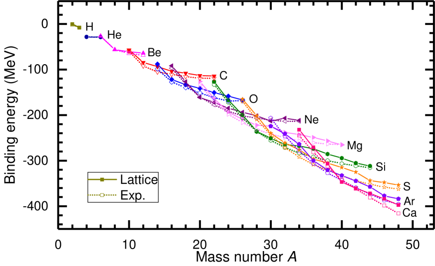
Figure 1: Nuclear binding energies. The calculated binding energies from ³H to ⁴⁸Ca. The solid symbols denote the lattice results and the open symbols denote the experimental values. Different symbols and colors denote different element. The Coulomb interaction is taken into account perturbatively. The experimental values are taken from Ref. Wang:2017 .

We now calculate the binding energies for 86 bound even-even nuclei (even number of protons, even number of neutrons) with up to $A=48$ nucleons. The results are shown and compared with empirical data in Fig. 1. Because the interaction has an exact SU(4) symmetry, we are free of the sign problem and can calculate the binding energies with high precision. In Fig. 1 all of the Monte Carlo error bars are smaller than the size of the symbols. The remaining errors due to imaginary time and volume extrapolations are also small, less than 1% relative error, and thus are also not explicitly shown. In Fig. 1 we see that the general trends for the binding energies along each isotopic chain are well reproduced. In particular, the isotopic curves on the proton-rich side are close to the experimental results. The discrepancy is somewhat larger on the neutron-rich side and is a sign of missing effects such as spin-dependent interactions.

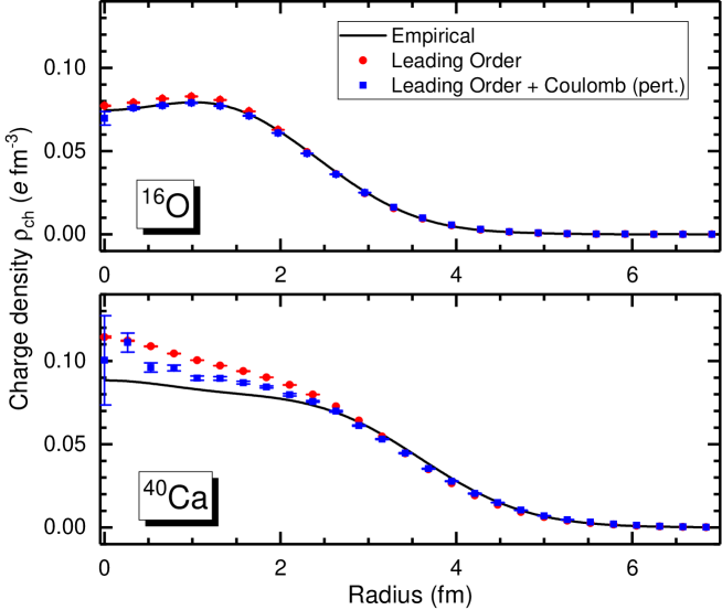
Figure 2: Charge density distributions. The calculated ¹⁶O and ⁴⁰Ca charge densities compared with the empirical results. The circles denote the results without Coulomb interaction. The squares denote the results with the Coulomb interaction included perturbatively. Empirical values are taken from Ref. DeVries:1987 .

The charge density profile is another important probe of nuclear structure. In Fig. 2 we show the charge densities of ¹⁶O and ⁴⁰Ca calculated with the pinhole algorithm. We have again taken into account the charge distribution of the proton. To compare with data from the electron scattering experiments we also show results with the Coulomb interaction included via first order perturbation theory. The Coulomb force suppresses the central densities, drawing the results closer to the empirical data. Our results are quite accurate for such a simple nuclear interaction.

We also examine the predictions for pure neutron matter (NM). In Fig. 3 we show the calculated NM energy as a function of the neutron density and the comparison with other calculations using next-to-next-to-next-to-leading-order (N³LO) chiral interactions. In the lattice results we vary the number of neutrons from 14 to 66. The data for three different box sizes $L$=5 (upright triangles), $L$=6 (squares), $L$=7 (rightward-pointing triangles) are marked as filled red polygons. We see that our results are in general agreement with the other calculations at densities above 0.05 fm^-3, though calculations at higher orders are needed and are planned in future work to estimate uncertainties. At lower densities the discrepancy is larger as a result of our SU(4)-invariant interaction having the incorrect neutron-neutron scattering length. The open red polygons, again $L$=5 (upright triangles), $L$=6 (squares), $L$=7 (rightward-pointing triangles), show an improved calculation with a short-range interaction to reproduce the physical neutron-neutron scattering length as well as a correction to improve invariance under Galilean boosts. The restoration of Galilean invariance on the lattice is described in Ref. Li:2019ldq . Overall, the results are quite good in view of the simplicity of the four-parameter interaction.

In this letter we have shown that the ground state properties of light nuclei, medium-mass nuclei, and neutron matter can be described using a minimal nuclear interaction with only four interaction parameters. While the first three parameters are already standard in $\chi$EFT, the fourth and last parameter is a new feature that controls the strength of the local part of the nuclear interactions. These insights can help design $\chi$EFT interactions with better convergence at higher densities. We encourage others to test simplified interactions in continuum nuclear structure calculations, interactions with SU(4) symmetry and a combination of local and nonlocal smearing. The details of our interaction are given in the Supplemental Material. In the continuum calculations, however, one can construct interactions with exact Galilean invariance, something that needs to be corrected order by order on the lattice Li:2019ldq .

We are now using SU(4)-symmetric short-range interactions with local and nonlocal smearing and also one-pion exchange as the starting point for improved calculations of light and medium-mass nuclei with chiral forces up to N³LO. While our ongoing N³LO work is far from finished, we do know that the corrections at NLO are typically at the 10% level in the binding energies. We should clarify that what we called LO in lattice chiral effective field theory is actually an improved LO calculation where the S-wave effective range correction is included. If the S-wave effective range correction were not included at LO, then the NLO correction would be at the 30% level. This 10% correction at NLO might still seem too large since the agreement between the LO results in this work and the experimental binding energies are better than 10%. However, this better-than-expected agreement can be explained by the additional fine-tuning we gain by adjusting the balance between local and nonlocal interactions to achieve accurate liquid drop properties.

The main takeaway message of the work presented here is that while some fine tuning of the chiral forces seems necessary to improve convergence at higher densities, the number of independent fine tunings does not appear to be large. While we have not solved the convergence problem, we characterized the scope of problem. The key remaining question is how to accomplish these fine tunings without fitting to the many-body data that we wish to predict. We plan to address this question in a forthcoming publication.

Aside from the Coulomb interaction, all of the other interactions in our minimal model respect Wigner’s SU(4) symmetry. This is an example of emergent symmetry. The SU(4)-invariant interaction resurges at higher densities not because the underlying fundamental interaction is exactly invariant, but because the SU(4)-invariant interaction is coherently enhanced in the many-body environment. This is not to minimize the important role of spin-dependent effects such as spin-orbit couplings and tensor forces. However, it does seem to suggest that SU(4) invariance plays a key role in the bulk properties of nuclear matter.

The computational effort needed for the auxiliary-field lattice Monte Carlo simulations scales with the number of nucleons, $A$, as somewhere between $A^{1}$ to $A^{2}$ for medium mass nuclei. The actual exponent depends on the architecture of the computing platform. The SU(4)-invariant interaction provides an enormous computational advantage by removing sign oscillations from the lattice Monte Carlo simulations for any even-even nucleus. Coulomb interactions and all other corrections can be implemented using perturbation theory or the recently-developed eigenvector continuation method if the corrections are too large for perturbation theory Frame:2017fah . Given the mild scaling with nucleon number and suppression of sign oscillations, the methods presented here provide a new route to realistic lattice simulations of heavy nuclei in the future with as many as one or two hundred nucleons. By realistic calculations we mean calculations where one can demonstrate order-by-order convergence in the chiral expansion going from LO to NLO, NLO to N²LO, and N²LO to N³LO, while maintaining agreement with empirical data.

We thank A. Schwenk for providing the neutron matter results for comparison. We acknowledge partial financial support from the Deutsche Forschungsgemeinschaft (SFB/TRR 110, “Symmetries and the Emergence of Structure in QCD”), the BMBF (Grant No. 05P15PCFN1), the U.S. Department of Energy (DE-SC0018638 and DE-AC52-06NA25396), and the Scientific and Technological Research Council of Turkey (TUBITAK project no. 116F400). Further support was provided by the Chinese Academy of Sciences (CAS) President’s International Fellowship Initiative (PIFI) (grant no. 2018DM0034) and by VolkswagenStiftung (grant no. 93562). The computational resources were provided by the Julich Supercomputing Centre at Forschungszentrum Jülich, Oak Ridge Leadership Computing Facility, RWTH Aachen, and Michigan State University.

Figure 3: Pure neutron matter. The pure neutron matter (NM) energy as a function of neutron density calculated using the NL50 interaction with box size $L$=5 (upright triangles), $L$=6 (squares), $L$=7 (rightward-pointing triangles), respectively. The filled red polygons show results for the leading-order SU(4)-symmetric interaction. The open red polygons show an improved calculation with a short-range interaction to reproduce the physical neutron-neutron scattering length as well as a correction to improve invariance under Galilean boosts. For comparison we also show results calculated with full N³LO chiral interactions (EM 500 MeV, EGM 450/500 MeV and EGM 450/700 MeV) Tews:2012fj , the results from variational (APR) Akmal:1998cf and Auxiliary Field Diffusion MC calculations (GCR) Gandolfi:2011xu .

I Supplemental Material

Auxiliary field formalism

We simulate the interactions of nucleons on the lattice using projection Monte Carlo with auxiliary fields; see Ref. Lee:2008fa ; Lahde:2019npb for an overview of methods used in lattice EFT. We use an auxiliary-field formalism where the interactions among nucleons are replaced by interactions of nucleons with auxiliary fields at every lattice point in space and time. In the auxiliary-field formalism each nucleon evolves as if it is a single particle in a fluctuating background of auxiliary fields. We use a single auxiliary field at LO in the EFT expansion coupled to the total nucleon density. The interactions are reproduced by integrating over the auxiliary field. In our lattice simulations, the spatial lattice spacing is taken to be $a$ = (150 MeV)^-1= 1.32 fm, and the time lattice spacing is $a_{t}$ = (1000 MeV)^-1= 0.197 fm. For any fixed initial and final state, the amplitude for a given configuration of auxiliary field is proportional to the determinant of an $A\times A$ matrix $M_{ij}$. The entries of $M_{ij}$ are the single nucleon amplitudes for a nucleon starting at state $j$ at $\tau$ = 0 and ending at state $i$ at $\tau$ = $\tau_{f}$.

We use a discrete auxiliary field that can simulate the two-, three- and four-body forces simultaneously without sign oscillations. To this end we write the interactions in the form,

$$:\exp\left(-\frac{1}{2}Ca_{t}\rho^{2}-\frac{1}{6}C_{3}a_{t}\rho^{3}-\frac{1}{24}C_{4}a_{t}\rho^{4}\right):=\sum_{k=1}^{N}\omega_{k}:\exp\left(\sqrt{-Ca_{t}}\phi_{k}\rho\right):,$$ (4)

where $C$ is the two-body coefficient, $C_{3}$ is three-body coefficient, $C_{4}$ is the four-body coefficient, and the :: symbols indicate the normal ordering of operators. We then solve for the real numbers $\omega_{k}$ and $\phi_{k}$. In this work we only consider attractive two-body interactions with $C<0$. In order to avoid the sign problem we further require $\omega_{k}>0$ for all $k$.

To determine the constants $\phi_{k}$ and $\omega_{k}$, we expand Eq. (4) up to $\mathcal{O}(\rho^{4})$ and compare both sides order by order. In the context of the nuclear EFT, the three- and four-body interactions are usually much weaker than the two-body interaction, and we use the following ansatz with $N=3$,

$$\omega_{1}=\frac{1}{\phi_{1}(\phi_{1}-\phi_{3})},\qquad\omega_{2}=1+\frac{1}{\phi_{1}\phi_{3}},\qquad\omega_{3}=\frac{1}{\phi_{3}(\phi_{3}-\phi_{1})}$$ (5)

where $\phi_{2}=0$ and $\phi_{1}$ and $\phi_{3}$ are two roots of the quadratic equation,

$$\phi^{2}+\frac{C_{3}}{\sqrt{-C^{3}a_{t}}}\phi-\frac{C_{3}^{2}}{C^{3}a_{t}}+\frac{C_{4}}{C^{2}a_{t}}-3=0.$$ (6)

Using Vieta’s formulas relating polynomial coefficients to the sums and products of roots, it is straightforward to verify that Eq. (5) satisfies Eq. (4) up to $\mathcal{O}(\rho^{4})$. For a pure two-body interaction with $C_{3,4}=0$, the solution is simplified to $\phi_{1}=-\phi_{3}=\sqrt{3}$, $\phi_{2}=0$, $\omega_{1}=\omega_{3}=1/6$, $\omega_{2}=2/3$. The formalism Eq. (5) is very efficient for simulating the many-body forces. The corresponding auxiliary field $s(n_{t},\bm{n})$ only assume three different values $\phi_{1}$, $\phi_{2}$ and $\phi_{3}$ and can be sampled with the shuttle algorithm described below.

Shuttle algorithm

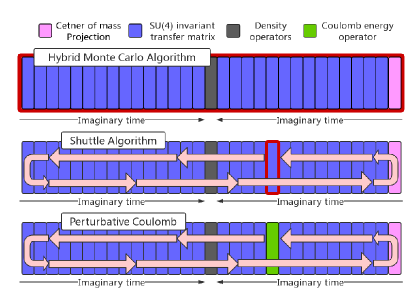
Figure S1: Update algorithms. The schematic plot for the HMC algorithm (upper panel), shuttle algorithm (middle panel) and the pinhole algorithm with a perturbative Coulomb force. The red squares denote the time slices to be updated in each run.

We update the auxiliary field $s(n_{t},\bm{n})$ using a shuttle algorithm where only one time slice is updated at a time. In Fig. S1 we show a schematic plot sketching the difference between the shuttle algorithm and the Hybrid Monte Carlo (HMC) algorithm which performs an update of all time slices. The shuttle algorithm works as follows. 1) Choose one time slice $n_{t}$, record the corresponding auxiliary field as $s_{{\rm old}}(n_{t},\bm{n}$). 2) Propose the new auxiliary fields $s_{{\rm new}}(n_{t},\bm{n}$) at each lattice site $\bm{n}$ according to the probability distribution $P\left[s_{{\rm new}}(n_{t},\bm{n})=\phi_{k}\right]=\omega_{k}$ for $k=1,2,3$. We note that $\omega_{1}+\omega_{2}+\omega_{3}=1$. 3) Calculate the determinant of the $A\times A$ correlation matrix $M_{ij}$ using $s_{{\rm old}}(n_{t},\bm{n})$ and $s_{{\rm new}}(n_{t},\bm{n})$, respectively. 4) Generate a random number $r\in[0,1)$ and perform the following “Metropolis test”. If

$$\left|\frac{\det\left[M_{ij}\left(s_{{\rm new}}(n_{t},\bm{n})\right)\right]}{\det\left[M_{ij}\left(s_{{\rm old}}(n_{t},\bm{n})\right)\right]}\right|>r,$$

accept the new configuration $s_{{\rm new}}(n_{t},\bm{n})$ and update the wave functions accordingly, otherwise keep $s_{{\rm old}}(n_{t},\bm{n})$. 5) Proceed to the next time slice, repeat steps 1)-4), and turn around at the end of the time series. As shown in Fig.S1, the program runs back-and-forth like a shuttle bus and all the auxiliary fields are updated after one cycle is finished.

The shuttle algorithm is well suited for small values of the temporal lattice spacing $a_{t}$. In this case the number of time slices is large and the impact of a single update is small. In each update the new configuation is close to the old one, resulting in a high acceptance rate. For example, in this work the temporal lattice spacing is $a_{t}=0.001$ MeV^-1 and the accept rate is around 50% in most cases. We compared the results with the HMC algorithm and found that the new algorithm is more efficient. In most cases the number of independent configurations per hour generated by the shuttle algorithm is three or four times larger than that generated by the HMC algorithm.

Charge densities with Coulomb

Auxiliary-field Monte Carlo simulations are efficient for computing the quantum properties of systems with attractive pairing interactions. By calculating the exact quantum amplitude for each configuration of auxiliary fields, we obtain the full set of correlations induced by the interactions. However, the exact quantum amplitude for each auxiliary field configuration involves quantum states which are superpositions of many different center-of-mass positions. Therefore information about density correlations relative to the center of mass is lost. Here we use the recently-developed pinhole algorithm to calculate the charge density profiles in the center-of-mass frame. The details of the algorithm can be found in Ref. Elhatisari:2017eno .

Let $\bm{n}_{k}=(\bm{r}_{k},s_{k},i_{k})$ denote the spatial coordinate, spin and isospin of nucleon $k$. The one-body density at a point $\bm{r}$ in the intrinsic frame can be written as

$$\langle\rho(r)\rangle =\frac{1}{A!}\sum_{\bm{n}_{1},\bm{n}_{2},\cdots,\bm{n}_{A}}\langle\Psi_{g.s.}|\rho_{A}|\Psi_{g.s.}\rangle\sum_{k=1}^{A}\delta(r-|\bm{r}_{k}-\bm{R}|)$$ (7)

where $\bm{R}=\frac{1}{A}\sum_{k}\bm{r}_{k}$ is the center of mass of $A$ nucleons, $|\Psi_{g.s.}\rangle$ is the ground state, $\rho_{A}=:\rho(\bm{n}_{1})\rho(\bm{n}_{2})\cdots\rho(\bm{n}_{A}):$ is the $A$-body density operator. The summation over $\bm{n}$ means a summation over all quantum numbers $\bm{n}_{1}$, $\bm{n}_{2}$, $\cdots$, $\bm{n}_{A}$.

The ground state $|\Psi_{g.s.}\rangle$ can be rewritten using the projection method,

$$|\Psi_{g.s.}\rangle=\lim_{L_{t}\rightarrow\infty}M^{L_{t}}|\Psi\rangle,\qquad M=:\exp(-a_{t}H):,$$

where $H$ is the Hamiltonian, $M$ is the tranfer matrix. Then Eq. (7) can be expressed using transfer matrices as

$$\langle\rho(r)\rangle=\frac{\sum_{\bm{n}}\langle\Psi|M^{L_{t}/2}\rho_{A}(\bm{n})M^{L_{t}/2}|\Psi\rangle\sum_{k=1}^{A}\delta(r-|\bm{r}_{k}-\bm{R}|)}{\sum_{\bm{n}}\langle\Psi|M^{L_{t}/2}\rho_{A}(\bm{n})M^{L_{t}/2}|\Psi\rangle}.$$ (8)

For the full Hamiltonian including Coulomb, Eq. (8) can not be computed directly using the Monte Carlo method because the repulsive Coulomb interaction induces sign oscillations. To solve this problem we employ perturbation theory. We split the Hamiltonian into two parts,

$$H=H^{(0)}+H^{(1)},$$

where $H^{(0)}$ is the leading order Hamiltonian consisting of the kinetic energy term and the SU(4)-invariant contact interactions, and $H^{(1)}$ stands for the Coulomb interaction. In what follows we only keep terms linear in $H^{(1)}$ or $M^{(1)}$ and omit all the higher order terms. The transfer matrix can be split similarly,

$$M=:\exp(-a_{t}H):=:\exp(-a_{t}H^{(0)}):-a_{t}:\exp(-a_{t}H^{(0)})H^{(1)}:=M^{(0)}+M^{(1)}.$$

Up to $\mathcal{O}(M^{(1)})$ the density Eq. (8) can be written as

$$\langle\rho(r)\rangle =\frac{\mathcal{M}_{\rho}^{(0)}+\mathcal{M}_{\rho}^{(1)}}{\mathcal{M}^{(0)}+\mathcal{M}^{(1)}}=\frac{\mathcal{M}_{\rho}^{(0)}}{\mathcal{M}^{(0)}}+\left(\frac{\mathcal{M}_{\rho}^{(1)}}{\mathcal{M}^{(0)}}-\frac{\mathcal{M}_{\rho}^{(0)}\mathcal{M}^{(1)}}{(\mathcal{M}^{(0)})^{2}}\right)+\mathcal{O}\left((\text{$\mathcal{M}$}^{(1)})^{2}\right),$$

where the amplitudes $\mathcal{M}^{(0)}$ and $\mathcal{M}_{\rho}^{(0)}$ are defined as

$$\mathcal{M}^{(0)} =\sum_{\bm{n}}\langle\Psi|(M^{(0)})^{L_{t}}|\Psi\rangle,$$

$$\mathcal{M}_{\rho}^{(0)} =\sum_{\bm{n}}\langle\Psi|(M^{(0)})^{L_{t}/2}\rho_{A}(\bm{n})(M^{(0)})^{L_{t}/2}|\Psi\rangle\sum_{k=1}^{A}\delta(r-|\bm{r}_{k}-\bm{R}|).$$

$\mathcal{M}^{(1)}$ and $\mathcal{M}_{\rho}^{(1)}$ are obtained by substituting one of the transfer matrices $M^{(0)}$ in $\mathcal{M}^{(0)}$ and $\mathcal{M}_{\rho}^{(0)}$ by $M^{(1)}$ and adding up all $L_{t}$ possibilities,

$$\mathcal{M}^{(1)} =\sum_{\bm{n}}\sum_{n_{t}=0}^{L_{t}/2-1}\langle\Psi|(M^{(0)})^{L_{t}-n_{t}-1}M^{(1)}(M^{(0)})^{n_{t}}|\Psi\rangle+{\rm c.c.},$$

$$\mathcal{M}_{\rho}^{(1)} =\sum_{\bm{n}}\sum_{n_{t}=0}^{L_{t}/2-1}\langle\Psi|(M^{(0)})^{L_{t}/2}\rho_{A}(\bm{n})(M^{(0)})^{L_{t}/2-n_{t}-1}M^{(1)}(M^{(0)})^{n_{t}}|\Psi\rangle\sum_{k=1}^{A}\delta(r-|\bm{r}_{k}-\bm{R}|)+{\rm c.c.}.$$

The four amplitudes $\mathcal{M}^{(0)}$, $\mathcal{M}^{(1)}$, $\mathcal{M}_{\rho}^{(0)}$ and $\mathcal{M}_{\rho}^{(1)}$ can be calculated using the auxiliary-field formalism described above.

SU(4) breaking effects

Our leading-order interactions fully respect Wigner’s SU(4) symmetry, but this symmetry is only approximate in nature. In order to optimize the strength of our SU(4) interaction, we calculate the energies of ³H and ⁴He using interactions corresponding to different scattering lengths $a_{0}$ with fixed effective range $r_{0}=2.2$ fm. The results are shown in Fig. S2 as full symbols. For each interaction we include the leading-order SU(4) breaking effects for the two $S$-wave channels adjusted to reproduce the experimental scattering lengths $a(^{1}$S${{}_{0}})$ and $a(^{3}$S${{}_{1}})$. The corrected energies are calculated using 1st order perturbation theory and shown as open symbols. The smaller values of $a_{0}$ correspond to stronger interactions and larger binding energies. From Fig. S2 we can see immediately that the energy corrections for ³H and ⁴He are both minimized at $a_{0}=9.1$ fm. We take this value for all of our calculations. This corresponds to a deuteron binding energy of $B(^{2}$H$)=0.677$ MeV.

Volume and surface constants

In this section we present the method for determining the parameter $s_{NL}$. For each value of $s_{NL}$ we repeat entire process of fitting $a_{0}=9.1$ fm, $r_{0}=2.2$ fm, and $B(^{3}$H$)=8.48$ MeV. Each time this process results in different values for the local smearing parameter $s_{L}$. We obtain five such interactions with $s_{NL}=$0.40, 0.45, 0.50, 0.55 and 0.60 and denote them as NL40, NL45, NL50, NL55, and NL60, respectively. We note that since the effective range is kept constant, decreasing $s_{NL}$ corresponds to increasing $s_{L}$ and thus the range of the local part of the interaction. While we used alpha-alpha scattering to fix the local part of the interaction in Ref. Elhatisari:2016owd , we are aware that such scattering calculations are difficult for other ab initio methods to reproduce. Therefore we adopt a different approach that looks at the ground state energies of medium mass nuclei.

For medium mass nuclei with $A\geq 16$, the binding energies can be well parameterized with the Bethe-Weizsäcker mass formula,

$$B(A)=a_{V}A-a_{S}A^{\frac{2}{3}}+E_{{\rm Coulomb}}+\cdots,$$ (9)

where $a_{V}$ and $a_{S}$ are volume-energy and surface-energy constants, respectively, $E_{{\rm Coulomb}}$ is the Coulomb energy, and the ellipsis represents other terms such as the symmetry energy, pairing energy, shell correction energy, etc. To avoid fitting complexities not accurately captured in our minimal nuclear interaction, we fit only $N=Z$ even-even nuclei, for which the symmetry energy vanishes and the pairing energy varies smoothly. The shell correction energy is known to be much smaller than the macroscopic contribution in this mass region Moller:1995 and thus the first three terms appearing in Eq. (9) dominate.

For each interaction we use the calculated binding energies with $16\leq A\leq 40$ to extract the liquid drop constants $a_{V}$ and $a_{S}$. We observe prominent shell effects for these nuclei, and the binding energy per nucleon fluctuates around the liquid drop values with maxima at the magic numbers. In the fitting procedure the shell effects across many nuclei averaged out, thus decreasing uncertainties for the liquid drop constants. The $a_{S}$-$a_{V}$ plot is shown in Fig. S3. We can see a linear correlation between these constants. The values of $a_{S}$ and $a_{V}$ both increase as the strength of the local part of the interaction increases. For comparison, we also show other values of these constants in the literature where the masses are fitted throughout the entire chart of nuclides. We find that the interaction NL50 gives a value of $a_{V}$ closest to the other estimations and corresponds to about 16 MeV binding energy per nucleon at saturation. The uncertainty in $a_{S}$ is large but still matches the empirical values.

Data extrapolation and error analysis

The Monte Carlo errors are calculated with a jackknife analysis. As we employ a leading-order action free from sign oscillations, in most cases the relative errors from the Monte Carlo simulation are smaller than 1% and are not shown explicitly in the figures. The only exceptions are the ⁴⁰Ca charge density with Coulomb included shown in the lower panel of Fig. 3, where the Monte Carlo errors become noticeable at small radii.

In all the calculations in this letter we use a fixed number of temporal steps $L_{t}$=300. The exact ground state energies can be obtained by extrapolating to the limit $L_{t}\rightarrow\infty$. To estimate the residual errors from using a finite $L_{t}$, we perform multiple calculations with $L_{t}$ varying from 100 to 300 for the nuclei listed in Table I. The results are used to fit to the ansatz,

$$E(L_{t})=E_{0}+c_{0}\exp\left(-\Delta EL_{t}a_{t}\right),$$

where $E_{0}$, $c_{0}$ and $\Delta E$ are fit parameters. The differences between the extrapolated energy $E_{0}$ and $E(L_{t}=300)$ are the time extrapolation errors shown in Table I.

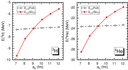
Figure S2: Binding energies of ³H and ⁴He. The solid symbols denote the binding energies of ³H and ⁴He calculated with leading order interactions fitted to different scattering length $a_{0}$ and fixed effective range $r_{0}=2.2$ fm. The open symbols denote the results with the leading order SU(4) breaking corrections fully included. See the text for details.

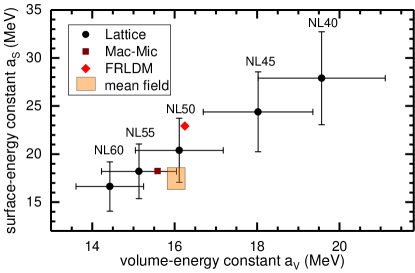
Figure S3: Volume/Surface energy constants. The correlation plot for the calculated volume-energy constant $a_{V}$ and surface-energy constant $a_{S}$. The square, diamond and square region denote the results fitted with Macroscopic-Microscopic model Wang:2014qqa , Finite Range Liquid Drop Model Moller:1995 , Mean Field Models Bender:2003jk , respectively.

References

- (1) E. Epelbaum, H. W. Hammer and U.-G. Meißner, Rev. Mod. Phys. 81, 1773 (2009).
- (2) R. Machleidt and D. R. Entem, Phys. Rept. 503, 1 (2011).
- (3) G. Hupin, S. Quaglioni and P. Navrátil, Phys. Rev. Lett. 114, no. 21, 212502 (2015).
- (4) P. Navrátil, V. G. Gueorguiev, J. P. Vary, W. E. Ormand, A. Nogga and S. Quaglioni, Few Body Syst. 43, 129 (2008).
- (5) D. Lonardoni, J. Carlson, S. Gandolfi, J. E. Lynn, K. E. Schmidt, A. Schwenk and X. Wang, Phys. Rev. Lett. 120, no. 12, 122502 (2018).
- (6) M. Piarulli et al., Phys. Rev. Lett. 120, no. 5, 052503 (2018).
- (7) E. Epelbaum et al. [LENPIC Collaboration], Phys. Rev. C 99, no. 2, 024313 (2019).
- (8) M. Wloch, D. J. Dean, J. R. Gour, M. Hjorth-Jensen, K. Kowalski, T. Papenbrock and P. Piecuch, Phys. Rev. Lett. 94, 212501 (2005).
- (9) G. Hagen, T. Papenbrock, D. J. Dean and M. Hjorth-Jensen, Phys. Rev. Lett. 101, 092502 (2008).
- (10) G. Hagen, M. Hjorth-Jensen, G. R. Jansen, R. Machleidt and T. Papenbrock, Phys. Rev. Lett. 108, 242501 (2012).
- (11) S. Binder, J. Langhammer, A. Calci and R. Roth, Phys. Lett. B 736, 119 (2014).
- (12) E. Epelbaum, H. Krebs, T. A. Lähde, D. Lee, U.-G. Meißner and G. Rupak, Phys. Rev. Lett. 112, no. 10, 102501 (2014).
- (13) A. Cipollone, C. Barbieri and P. Navrátil, Phys. Rev. C 92, no. 1, 014306 (2015).
- (14) A. Ekström et al., Phys. Rev. C 91, no. 5, 051301 (2015) doi:10.1103/PhysRevC.91.051301 [arXiv:1502.04682 [nucl-th]].
- (15) U.-G. Meißner, J. A. Oller and A. Wirzba, Annals Phys. 297, 27 (2002).
- (16) A. Lacour, J. A. Oller and U.-G. Meißner, Annals Phys. 326, 241 (2011).
- (17) G. Hagen et al., Nature Phys. 12, no. 2, 186 (2015).
- (18) G. Hagen, G. R. Jansen and T. Papenbrock, Phys. Rev. Lett. 117, no. 17, 172501 (2016).
- (19) J. Simonis, S. R. Stroberg, K. Hebeler, J. D. Holt and A. Schwenk, Phys. Rev. C 96, no. 1, 014303 (2017).
- (20) T. D. Morris et al., Phys. Rev. Lett. 120, no. 15, 152503 (2018).
- (21) S. Elhatisari et al., Phys. Rev. Lett. 117, no. 13, 132501 (2016).
- (22) E. Wigner, Phys. Rev. 51, 106 (1937).
- (23) A. Calle Cordon and E. Ruiz Arriola, Phys. Rev. C 80, 014002 (2009) doi:10.1103/PhysRevC.80.014002 [arXiv:0904.0421 [nucl-th]].
- (24) L. Platter, H.-W. Hammer and U.-G. Meißner, Phys. Lett. B 607, 254 (2005) doi:10.1016/j.physletb.2004.12.068 [nucl-th/0409040].
- (25) N. Klein, S. Elhatisari, T. A. Lähde, D. Lee and U.-G. Meißner, Eur. Phys. J. A 54, no. 7, 121 (2018).
- (26) S. König, H. W. Grießhammer, H. W. Hammer and U. van Kolck, Phys. Rev. Lett. 118, no. 20, 202501 (2017).
- (27) A. Kievsky and M. Gattobigio, Few Body Syst. 57, no. 3, 217 (2016).
- (28) S. Elhatisari et al., Phys. Rev. Lett. 119, no. 22, 222505 (2017).
- (29) A. Rokash, E. Epelbaum, H. Krebs and D. Lee, Phys. Rev. Lett. 118, no. 23, 232502 (2017).
- (30) N. Klein, D. Lee and U.-G. Meißner, Eur. Phys. J. A 54, no. 12, 233 (2018).
- (31) B. N. Lu, T. A. Lähde, D. Lee and U.-G. Meißner, Phys. Lett. B 760, 309 (2016).
- (32) D. Lee, Prog. Part. Nucl. Phys. 63, 117 (2009).
- (33) T. A. Lähde and U.-G. Meißner, Lect. Notes Phys. 957, 1 (2019).
- (34) M. Wang et al., Chin. Phys. C 41, 030003 (2017).
- (35) I. Angeli and K. P. Marinova, Atom. Data Nucl. Data Tabl. 99, no. 1, 69 (2013).
- (36) H. De Vries, C. W. De Jager, and C. De Vries, Atom. Data Nucl. Data Tabl. 36, 495 (1987).
- (37) I. Tews, T. Krüger, K. Hebeler and A. Schwenk, Phys. Rev. Lett. 110, no. 3, 032504 (2013).
- (38) A. Akmal, V. R. Pandharipande and D. G. Ravenhall, Phys. Rev. C 58, 1804 (1998).
- (39) S. Gandolfi, J. Carlson and S. Reddy, Phys. Rev. C 85, 032801 (2012).
- (40) N. Li, S. Elhatisari, E. Epelbaum, D. Lee, B. Lu and U. G. Meißner, Phys. Rev. C 99, no. 6, 064001 (2019).
- (41) D. Frame, R. He, I. Ipsen, D. Lee, D. Lee and E. Rrapaj, Phys. Rev. Lett. 121, no. 3, 032501 (2018).
- (42) N. Wang, M. Liu, X. Wu and J. Meng, Phys. Lett. B 734, 215 (2014).
- (43) P. Möller, J. R. Nix, W. D. Myers and W. J. Swiatecki, Atom. Data Nucl. Data Tabl. 59, 185 (1995).
- (44) M. Bender, P. H. Heenen and P. G. Reinhard, Rev. Mod. Phys. 75, 121 (2003).