Hill four-body problem with oblate tertiary: an application to the Sun-Jupiter-Hektor-Skamandrios system

Abstract.

We consider a restricted four-body problem with a precise hierarchy between the bodies: two point-mass bigger bodies, a smaller one with oblate shape, and an infinitesimal body in the neighborhood of the oblate body. The three heavy bodies are assumed to move in a plane under their mutual gravity, and the fourth body moves under the gravitational influence of the three heavy bodies, but without affecting them.

We start by finding the triangular central configurations of the three heavy bodies; since one body is oblate, the triangle is isosceles, rather than equilateral as in the point mass case. We assume that the three heavy bodies are in such a central configuration and we perform a Hill’s approximation of the equations of motion describing the dynamics of the infinitesimal body in a neighborhood of the oblate body. Through the use of Hill’s variables and a limiting procedure, this approximation amounts to sending the two other bodies to infinity. Finally, for the Hill approximation, we find the equilibrium points of the infinitesimal body and determine their stability. As a motivating example, we consider the dynamics of the moonlet Skamandrios of Jupiter’s Trojan asteroid Hektor.

1. Introduction

The discovery of binary asteroids has led to considering dynamical models formed by four bodies, two of them being typically the Sun and Jupiter. Among possible four-body models (see also [HS86, Sch98, GJ03, SB05, ARV09, BGD13b, BGD13a, BG16, KMJ17]), a relevant role is played by the models in which three bodies lie on a triangular central configuration. Given that asteroids have often a (very) irregular shape, it is useful to start by investigating the case in which one body has an oblate shape. Among the different questions that this model may rise, we concentrate on the existence of equilibrium points and the corresponding linear stability analysis. Within such framework, we consider a four-body simplified model and we concentrate on the specific example given by the Trojan asteroid 624 Hektor, which is located close to the Lagrangian point $L_{4}$ of the Sun-Jupiter system, and its small moonlet.

In our model Sun, Jupiter and Hektor form an isosceles triangle (nearly equilateral) whose shape remains unchanged over time. The small body represents Hektor’s moonlet Skamandrios. Obviously, we could also replace the moonlet by a spacecraft orbiting Hektor. The system Sun-Jupiter-Hektor-Skamandrios plays a relevant role for several reasons. Indeed, Hektor is the largest Jupiter Trojan, it has one of the most elongated shapes among the bodies of its size in the Solar system, and it is the only known Trojan to possess a moonlet (see, e.g., [DLZ12] for stability regions of Trojans around the Earth and [LC15] for dissipative effects around the triangular Lagrangian points).

The study of asteroids with satellites presents a special interest for planetary dynamics, as they provide information about constraints on the formation and evolution of the Solar system.

Another motivation to study the dynamics of a small body near a Trojan asteroid comes from astrodynamics, as NASA prepares the first mission, Lucy, to the Jupiter’s Trojans, which is planned to be launched in October 2021 and visit seven different asteroids: a Main Belt asteroid and at least five Trojans.

As a model for the Sun-Jupiter-Hektor dynamics, we consider a system of three bodies of masses $m_{1}\geq m_{2}\geq m_{3}$, which move in circular orbits under mutual gravity, and form a triangular central configuration. We refer to these bodies as the primary, the secondary, and the tertiary, respectively. We assume that the first two bodies of masses $m_{1},m_{2}$ are spherical and homogeneous, so they can be treated as point masses, while the third body of mass $m_{3}$ is oblate. We describe the gravitational potential of $m_{3}$ in terms of spherical harmonics, and we only retain the most significant ones. We show the existence of a corresponding triangular central configuration, which turns out to be an isosceles triangle; if the oblateness of the mass $m_{3}$ is made to be zero, the central configuration becomes the well-known equilateral triangle Lagrangian central configuration. We stress that when $m_{3}$ is oblate, the central configuration is not the same as in the non-oblate case, since the overall gravitational field of $m_{3}$ is no longer Newtonian; it is well known that central configurations depend on the nature of the gravitational field (see, e.g., [CLPC04, APC13, DSZ, MS17]). We note that there exist papers in the literature (e.g., [APHS16]), which consider systems of three bodies, with one of the bodies non-spherical, which are assumed to form an equilateral triangle central configuration. Such assumption, while it may lead to very good approximations, is not physically correct.

The moonlet Skamandrios is represented by a fourth body, of infinitesimal mass, which moves in a vicinity of $m_{3}$ under the gravitational influence of $m_{1},m_{2},m_{3}$, but without affecting their motion. We consider the motion of the infinitesimal mass taking place in the three-dimensional space; it is not restricted to the plane of motion of the three heavy bodies. This situation is referred to as the spatial circular restricted four-body problem, and can be described by an autonomous Hamiltonian system of $3$-degrees of freedom.

We ‘zoom-in’ onto the dynamics in a small neighborhood of $m_{3}$ by performing a Hill’s approximation of the restricted four-body problem. This is done by a rescaling of the coordinates in terms of $m_{3}^{1/3}$, writing the associated Hamiltonian in the rescaled coordinates as a power series in $m_{3}^{1/3}$, and neglecting all the terms of order $O(m_{3}^{1/3})$ in the expansion, since such terms are small when $m_{3}$ is small. This yields an approximation of the motion of the massless particle in an $O(m_{3}^{1/3})$-neighborhood of $m_{3}$, while $m_{1}$ and $m_{2}$ are ‘sent to infinity’ through the rescaling. This model is an extension of the classical lunar Hill problem [Hil78]. Since the tertiary is assumed to be oblate, and the corresponding central configuration formed by the three heavy bodies is not an equilateral triangle anymore, this model also extends Hill’s approximation of the restricted four-body problem developed in [BGG15].

The Hill approximation is more advantageous to utilize for this system than the restricted four-body problem, since it allows for an analytical treatment, and yields more accurate numerical implementations when realistic parameters are used. The main numerical difficulty in the restricted four-body problem is the large differences of scales among the relevant parameters, i.e. the mass of Hektor is much smaller than the masses of the other two heavy bodies. The rescaling of the coordinates involved in the Hill approximation reduces the difference of scales of the parameters to more manageable quantities; more precisely, in normalized units the oblateness effect in the restricted four-body problem is of the order $O(10^{-15})$, while in the Hill approximation is of the order $O(10^{-7})$ (see Section 3.2 for details).

Once we have established the model for the Hill four-body problem with oblate tertiary, we study the equilibrium points and their linear stability. We find that there are $2$ pairs of symmetric equilibrium points on each of the $x$-, $y$-, and $z$-coordinate axes, respectively. The equilibrium points on the $x$- and $y$-coordinate axes are just a continuation of the corresponding ones for the Hill four-body problem with non-oblate tertiary [BGG15]. The equilibrium points on the $z$-coordinate axis constitute a new feature of the model. In the case of Hektor, these equilibrium points turn out to be outside of the body of the asteroid but very close to the surface, so they are of potential interest for low altitude orbit space missions, such as the one of NASA/JPL’s Dawn mission around Vesta ([Del11]).

This work is organized as follows. In Section 2 we describe in full details the restricted four-body model in which the tertiary is oblate; in particular, we describe the isosceles triangle central configuration of three bodies in which two bodies are point masses and the third is oblate. Hill’s approximation is introduced in Section 3. The determination of the equilibria and their stability is given in Section 4.

2. Restricted four-body problem with oblate tertiary

In this section we develop a model for a restricted four-body problem, which consists of two bigger bodies (e.g., the Sun and Jupiter), a smaller body – called tertiary – with oblate shape (e.g. an asteroid), and an infinitesimal mass (e.g., moonlet) around the tertiary.

As mentioned in Section 1, we consider the three masses $m_{1}\geq m_{2}\geq m_{3}$ as moving under the mutual gravitational attraction; the bodies with masses $m_{1}$ and $m_{2}$ are considered as point masses, while $m_{3}$ is the oblate body. We normalize the units of mass so that $m_{1}+m_{2}+m_{3}=1$.

We assume that the bodies with masses $m_{1}$, $m_{2}$, $m_{3}$ move on a triangular central configuration, which will be determined in Section 2.3, once the gravitational field of the oblate body has been discussed in Section 2.2. We will concentrate on the specific example given by the asteroid Hektor and its moon Skamandrios, where Hektor moves on a central configuration with Jupiter and the Sun. Orbital and physical values are given in Section 2.1. The positions of the three man bodies in the triangular central configuration is computed in Section 2.4, while the equations of motion of the moonlet – with infinitesimal mass moving in the vicinity of $m_{3}$ – are given in Section 2.5.

2.1. Data on the Sun-Jupiter-Hektor-Skamandrios system

The models which we will develop below will be applied to the case of the Sun-Jupiter-Hektor-Skamandrios system. We extract the data for this system from [JPL, MDCR⁺14, Des15].

Hektor is approximately located at the Lagrangian point $L_{4}$ of the Sun-Jupiter system. According to [Des15], Hektor is approximately $416\times 131\times 120$ km in size, and its shape can be approximated by a dumb-bell figure; the equivalent radius (i.e., the radius of a sphere with the same volume as the asteroid) is $R_{H}=92$ km.

Hektor spins very fast, with a rotation period of approximately $6.92$ hours (see the JPL Solar System Dynamics archive [JPL]).

The moonlet Skamandrios orbits around Hektor at a distance of approximately $957.5$ km, with an orbital period of $2.965079$ days; see [Des15]. Its orbit is highly inclined, at approximately $50.1^{\circ}$ with respect to the orbit of Hektor, which justifies choosing as a model the spatial restricted four-body problem rather than the planar one; see [MDCR⁺14].

We also note that the inclination of Hektor is approximately $18.17^{\circ}$ (see [JPL]). Although a more refined model should include a non-zero inclination, we will consider that Sun-Jupiter-Hektor move in the same plane, an assumption that is needed in order for the three bodies to form a central configuration. We will further assume that the axis of rotation of Hektor is perpendicular to the plane of motion.

For the masses of Sun, Jupiter and Hektor we use the values of $m_{1}=1.989\times 10^{30}$ kg, $m_{2}=1.898\times 10^{27}$, and $m_{3}=7.91\times 10^{18}$ kg, respectively. For the average distance Sun-Jupiter we use the value $778.5\times 10^{6}$ km.

In Figure 1 we provide a comparison between the strength of the different forces acting on the moonlet: the Newtonian gravitational attraction of Hektor, Sun, Jupiter, and the effect of the non-spherical shape of the asteroid, limited to the the so-called $J_{2}$ coefficient, which will be introduced in Section 2.2.

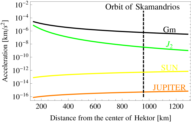
Figure 1. Order of magnitude of the different perturbations acting on the moonlet as a function of its distance from Hektor. The terms Gm, Sun and Jupiter denote, respectively, the monopole terms of the gravitational influence of Hektor, the attraction of the Sun and that of Jupiter. $J_{2}$ represents the perturbation due to the non-spherical shape of Hektor. The actual distance of the moonlet is indicated by a vertical line.

2.2. The gravitational field of a non-spherical body

We first consider that the tertiary body, representing Hektor, has a general (non-spherical) shape. The gravitational potential, relative to a reference frame centered at the barycenter of the tertiary and rotating with the body, is given in spherical coordinates $(r,\phi,\lambda)$ by (see, e.g., [CG18]):

$$V(r,\phi,\lambda)={{\mathcal{G}m_{H}}\over r}\ \sum_{n=0}^{\infty}\Bigl{(}{R_{H}\over r}\Bigr{)}^{n}\ \sum_{m=0}^{n}P_{nm}(\sin\phi)\ (C_{nm}\cos m\lambda+S_{nm}\sin m\lambda)\ ,$$

where $\mathcal{G}$ is the gravitational constant, $m_{H}$ is the mass of Hektor, $R_{H}$ is its average radius, $P_{nm}$ are the Legendre polynomials defined as

$$\begin{split}P_{n}(x)&={1\over{2^{n}n!}}\ {{d^{n}}\over{dx^{n}}}(x^{2}-1)^{n}\\ P_{nm}(x)&=(1-x^{2})^{m\over 2}\ {{d^{m}}\over{dx^{m}}}P_{n}(x)\ ,\end{split}$$

and $C_{nm}$ and $S_{nm}$ are the spherical harmonics coefficients.

In the case of an ellipsoid of semi-axes $a\geq b\geq c$, we have the following explicit formulas ([Boy97]):

$$S_{n,m} = 0,$$

$$C_{2p+1,2q} = 0,$$

$$C_{2p,2q+1} = 0,$$

$$C_{2p,2q} = \displaystyle{3\over{R_{H}^{2p}}}{{p!(2p-2q)!}\over{2^{2q}(2p+3)(2p+1)!}}(2-\delta_{0q})$$

$$\displaystyle\sum_{i=0}^{\lfloor{{p-q}\over 2}\rfloor}{{(a^{2}-b^{2})^{q+2i}[c^{2}-{1\over 2}(a^{2}+b^{2})]^{p-q-2i}}\over{16^{i}(p-q-2i)!(p+q)!i!}}.$$

In particular, $C_{20}$ and $C_{22}$ turn out to be given by simple expressions

(2.1) $$C_{20} = \frac{c^{2}-\frac{a^{2}}{2}-\frac{b^{2}}{2}}{5R_{H}^{2}},$$

(2.2) $$C_{22} = \frac{\frac{a^{2}}{4}-\frac{b^{2}}{4}}{5R_{H}^{2}}.$$

For the Sun-Jupiter-Hektor data, we take $a=208$ km, $b=65.5$ km, $c=60$ km, $R_{H}=92$ km, following [Des15] (see Section 2.1), we calculate the following coefficients:

$$C_{20}=-0.476775$$; ;

; ; ;

; ; ; .

Notice that each term $C_{2p,2q}$ is multiplied in (2.2) by the factor $R_{H}^{2p}/r^{2p+1}$. For $r$ equal to the average distance from the moonlet to the asteroid, we have $R_{H}/r\approx 0.096$. Therefore, in the following we will ignore the effect of the coefficients $C_{2p,2q}$, with $p\geq 2$, which are at least of $O(R_{H}^{4}/r^{5})$.

Note that the value of $C_{20}$ computed above is significantly bigger in absolute value than the one reported in [MDCR⁺14], which equals $-0.15$. The reason is that we use different estimates for the size of Hektor, following [Des15] (see Section 2.1).

If we consider a frame centered at the barycenter of the tertiary, and which rotates with the angular velocity of the tertiary about the primary, the time dependent gravitational potential takes of the form

$$V(r,\phi,\lambda)={{\mathcal{G}m_{H}}\over r}\ \sum_{n=0}^{2}\Bigl{(}{R_{H}\over r}\Bigr{)}^{n}\ \sum_{m=0}^{n}P_{nm}(\sin\phi)\ C_{nm}\cos(m(\lambda+\Theta t)),$$

where $\Theta$ represents the frequency of the spin of Hektor.

For $n=2$, $m=0$ the corresponding term $C_{nm}\cos(m(\lambda+\Theta t))$ in the summation (2.2) is equal to $C_{20}$ and is independent of time; for $n=2$, $m=2$ the corresponding term $C_{nm}\cos(m(\lambda+\Theta t))$ is equal to $C_{22}\cos(2(\lambda+\Theta t))$, so is time-dependent. We do not consider the other terms in the sum (2.2).

Since the ratio of the rotation period of Hektor to the orbital period of the moonlet is relatively small, approximately $0.09740991$, in this paper we will only consider the average effect of $C_{22}\cos(2(\lambda+\Theta t))$ on the moonlet, which is zero.

In conclusion, in the model below we will only consider the effect of $C_{20}:=-J_{2}<0$, which amounts to approximating Hektor as an oblate body (i.e., an ellipsoid of revolution obtained by rotating an ellipse about its minor axis); the dimensionless quantity $J_{2}$ is referred to as the zonal harmonic in the gravitational potential. The term corresponding to $C_{20}$ is the larger one, followed by that corresponding to $C_{22}$; however, since the $C_{22}$ term introduces a time dependence, thus further complicating the model, we start by disregarding it and plan to study its effect in a future work.

2.3. Central configurations for the three-body problem with one oblate body

We now consider only the three heavy bodies, of masses $m_{1}\geq m_{2}\geq m_{3}$, with the body of mass $m_{3}$ being oblate, in which case we only take into account the term corresponding to $C_{20}=-J_{2}$ in (2.2). We write the approximation of the gravitational potential of the tertiary (2.2) in both Cartesian and spherical coordinates (in the frame of the tertiary and rotating with the body):

(2.3) $$\begin{split}V(x,y,z)&=\frac{m_{3}}{r}-\frac{m_{3}}{r}\left(\frac{R_{3}}{r}\right)^{2}\left(\frac{J_{2}}{2}\right)\left(3\left(\frac{z}{r}\right)^{2}-1\right)\\ &=\frac{m_{3}}{r}+\frac{m_{3}}{r}\left(\frac{R_{3}}{r}\right)^{2}\left(\frac{C_{20}}{2}\right)\left(3\sin\phi^{2}-1\right),\end{split}$$

where $m_{3}$ is the normalized mass of Hektor (the sum of the three masses is the unit of mass), $R_{3}:=R_{H}$ is the average radius of Hektor in normalized units (the distance between Sun and Hektor is the unit of distance), the gravitational constant is normalized to $1$, and $\sin\phi=z/r$.

We want to find the triangular central configurations formed by $m_{1}$, $m_{2}$, $m_{3}$; we will follow the approach in [APC13]. Since for a central configuration the three bodies lie in the same plane, in the gravitational field (2.3) of $m_{3}$ we set $\phi=0$, obtaining

(2.4) $$V(q)=\frac{m_{3}}{r}+\frac{Cm_{3}}{r^{3}},$$

where $q=(x,y)$ is the position vector of an arbitrary point in the plane, $r=\|q\|$ is the distance from $m_{3}$, and we denote

(2.5) $$C=R_{3}^{2}J_{2}/2>0.$$

Let $q_{i}$ be the position vector of the mass $m_{i}$, for $i=1,2,3$, in an inertial frame centered at the barycenter of the three bodies.

The equations of motion of the three bodies are

(2.6) $$\begin{split}m_{1}\ddot{q}_{1}&={m_{1}m_{2}(q_{2}-q_{1})}\frac{1}{\|q_{2}-q_{1}\|^{3}}+{m_{1}m_{3}(q_{3}-q_{1})}\left[\frac{1}{\|q_{3}-q_{1}\|^{3}}+\frac{3C}{\|q_{3}-q_{1}\|^{5}}\right],\\ m_{2}\ddot{q}_{2}&={m_{2}m_{1}(q_{1}-q_{2})}\frac{1}{\|q_{1}-q_{2}\|^{3}}+{m_{2}m_{3}(q_{3}-q_{2})}\left[\frac{1}{\|q_{3}-q_{2}\|^{3}}+\frac{3C}{\|q_{3}-q_{2}\|^{5}}\right],\\ m_{3}\ddot{q}_{3}&={m_{3}m_{1}(q_{1}-q_{3})}\frac{1}{\|q_{1}-q_{3}\|^{3}}+{m_{3}m_{2}(q_{2}-q_{3})}\frac{1}{\|q_{2}-q_{3}\|^{3}},\end{split}$$

where the last terms in the first two equations are due to (2.4), and the gravitational constant is normalized to $\mathcal{G}=1$. Denote $r_{ij}=\|q_{i}-q_{j}\|$, for $i\neq j$, ${\bf q}=(q_{1},q_{2},q_{3})$, and ${\bf M}=\textrm{diag}(m_{1},m_{1},m_{2},m_{2},m_{3},m_{3})$ the $6\times 6$ matrix with $2$ copies of each mass along the diagonal. Then (2.6) can be written as

(2.7) $${{\bf M}}\ddot{{\bf q}}=\nabla U({\bf q}),$$

where

(2.8) $$U({\bf q})={m_{1}m_{2}}\frac{1}{r_{12}}+{m_{1}m_{3}}\left(\frac{1}{r_{13}}+\frac{C}{r_{13}^{3}}\right)+{m_{2}m_{3}}\left(\frac{1}{r_{23}}+\frac{C}{r_{23}^{3}}\right)$$

is the potential for the three body problem with oblate $m_{3}$.

Let us assume that the center of mass is fixed at the origin, i.e.,

(2.9) $${\bf M}{\bf q}=\sum_{i=1}^{3}m_{i}q_{i}=0.$$

We are interested in relative equilibrium solutions for the motion of the three bodies, which are characterized by the fact they become equilibrium points in a uniformly rotation frame.

Denote by $R(\theta)$ the $6\times 6$ block diagonal matrix consisting of $3$ diagonal blocks the form

$$\left(\begin{array}[]{rr}\cos(\theta)&-\sin(\theta)\\ \sin(\theta)&\cos(\theta)\\ \end{array}\right)\in SO(2).$$

Substituting ${\bf q}(t)=R(\omega t){\bf z}(t)$ for some $\omega\in\mathbb{R}$ in (2.7), where ${\bf z}=(z_{1},z_{2},z_{3})\in\mathbb{R}^{6}$, we obtain

$${\bf M}\left(\ddot{\bf z}+2\omega J\dot{\bf z}-\omega^{2}{\bf z}\right)=\nabla U,$$

where $J$ is the block diagonal matrix consisting of $3$ diagonal blocks the form

(2.10) $$\left(\begin{array}[]{rr}0&-1\\ 1&0\\ \end{array}\right).$$

The condition for an equilibrium point of (2.3) yields the algebraic equation

(2.11) $$\nabla U({\bf z})+\omega^{2}{\bf M}{\bf z}=0.$$

A solution ${\bf z}$ of the three-body problem satisfying (2.11) is referred to as a central configuration. This is equivalent to $\ddot{z}_{i}=-\omega^{2}z_{i}$, for $i=1,2,3$, meaning that the accelerations of the masses are proportional to the corresponding position vectors, and all accelerations are pointing towards the center of mass. Thus, the solution ${\bf q}(t)$ is a relative equilibrium solution if and only if ${\bf q}(t)=R(\omega t){\bf z}(t)$ with ${\bf z}(t)$ being a central configuration solution, and the rotation $R(\omega t)$ being a circular solution of the Kepler problem.

Let $I({\bf z})={\bf z}^{T}M{\bf z}=\sum_{i}m_{i}\|z_{i}\|^{2}$ be the moment of inertia. It is easy to see that this is a conserved quantity for the motion, that is, $I({\bf z}(t))=\bar{I}$ for some $\bar{I}$ at all $t$. Using Lagrange’s second identity (see, e.g., [GN12]), and that ${\bf M}{\bf z}=0$, normalizing the masses so that $\sum_{i=1}^{3}m_{i}=1$, the moment of inertia can be written as:

(2.12) $$I({\bf z})=\sum_{1\leq i<j\leq 3}m_{ij}\|z_{i}-z_{j}\|^{2}:=\sum_{1\leq i<j\leq 3}m_{ij}r_{ij}^{2}.$$

Thus, central configurations correspond to critical points of the potential $U$ on the sphere ${\bf z}^{T}M{\bf z}=1$, which can be obtained by solving the Lagrange multiplier problem

(2.13) $$\nabla f({\bf z})=0,\qquad I({\bf z})-\bar{I}=0,$$

where $f({\bf z})=U({\bf z})+\frac{1}{2}\omega^{2}(I({\bf z})-\bar{I})$. In the above, we used the fact that $\nabla I({\bf z})=2{\bf M}{\bf z}$.

We solve this problem in the variables $r_{ij}=\|z_{i}-z_{j}\|$ for $1\leq i<j\leq 3$, since both $U$ and $I$ can be written in terms of these variables. This reduces the dimension of the system (2.13) from $7$ equations to $4$ equations. Denote ${\bf r}=(r_{12},r_{13},r_{23})$, and let $\tilde{f}({\bf r})$ be the function $f$ expressed in the variable ${\bf r}$, that is $\tilde{f}({\bf r}({\bf z}))=f({\bf z})$. By the chain rule, $\nabla_{r}\tilde{f}\cdot\left(\frac{\partial{\bf r}}{\partial{\bf z}}\right)=\nabla_{\bf z}f({\bf z})$. It is easy to see that the rank of the matrix $\left(\frac{\partial{\bf r}}{\partial{\bf z}}\right)$ is maximal provided that $z_{1},z_{2},z_{3}$ are not collinear (for details, see [CLPC04, APC13]). As we are looking for triangular central configurations, this condition is satisfied. Thus, $\nabla_{r}\tilde{f}({\bf r})=0$ if and only if $\nabla_{\bf z}f({\bf z})=0$. In other words, we can now solve the system (2.13) in the variable ${\bf r}$. We obtain

(2.14) $$\begin{split}-\frac{1}{r_{12}^{2}}+\omega^{2}r_{12}=0,\\ -\frac{1}{r_{13}^{2}}-\frac{3C}{r_{13}^{4}}+\omega^{2}r_{13}=0,\\ -\frac{1}{r_{23}^{2}}-\frac{3C}{r_{23}^{4}}+\omega^{2}r_{23}=0,\\ m_{1}m_{2}r_{12}^{2}+m_{1}m_{3}r_{13}^{2}+m_{2}m_{3}r_{23}^{2}=\bar{I}.\end{split}$$

Note that the function $h(r)=-\frac{1}{r^{3}}-\frac{3C}{r^{5}}$ has positive derivative $h^{\prime}(r)=\frac{3}{r^{4}}+\frac{15C}{r^{6}}$ with $C,r>0$, hence it is injective. Thus, the second and third equation in (2.14) yield $r_{13}=r_{23}:=u$. Solving for $\omega$ in the first and second equation we obtain:

(2.15) $$\omega=\sqrt{\frac{1}{r_{12}^{3}}}=\sqrt{\frac{1}{r_{13}^{3}}+\frac{3C}{r_{13}^{5}}}.$$

Solving for $r_{12}$ yields:

(2.16) $$r_{12}:=v=\left(\frac{u^{5}}{u^{2}+3C}\right)^{1/3}.$$

Notice that $C>0$ implies $0<v<u$.

The condition $I({\bf r})=\bar{I}$ yields

$$m_{1}m_{2}\left(\frac{u^{5}}{u^{2}+3C}\right)^{2/3}+(m_{1}m_{3}+m_{2}m_{3})u^{2}=\bar{I},$$

which is equivalent to

$$\frac{m_{1}^{3}m_{2}^{3}u^{10}}{\left(u^{2}+3C\right)^{2}}=\left(\bar{I}-(m_{1}m_{3}+m_{2}m_{3})u^{2}\right)^{3}.$$

To simplify the notation, let $u^{2}=z$, $m_{1}^{3}m_{2}^{3}=a$, $m_{1}m_{3}+m_{2}m_{3}=c$, $3C=b$, obtaining

$$\frac{az^{5}}{(z+b)^{2}}=(\bar{I}-cz)^{3}.$$

The function $k(z)=\displaystyle\frac{az^{5}}{(z+b)^{2}}$ has derivative

$$k^{\prime}(z)=\frac{3az^{6}+8abz^{5}+5ab^{2}z^{4}}{(z+b)^{4}}>0$$

and the function $l(z)=(\bar{I}-cz)^{3}$ has derivative

$$l^{\prime}(z)=-3c(\bar{I}-cz)^{2}<0.$$

Since

$$k(0)=0\textrm{ and }\lim_{z\to+\infty}k(z)=+\infty,$$

and

$$l(0)=\bar{I}^{3}>0\textrm{ and }\lim_{z\to+\infty}l(z)=-\infty,$$

the equation $k(z)=l(z)$ has a unique solution with $z>0$. We conclude that for each fixed $\bar{I}$, there is a unique solution of (2.14). Thus, we have proved the following result.

Proposition 2.1.

In the three-body problem with one oblate primary, for every fixed value $\bar{I}$ of the moment of inertia there exists a unique central configuration, which is an isosceles triangle.

We note that, while [APC13] studies central configurations of three oblate bodies (as well as of three bodies under Schwarzschild metric), the isosceles central configuration found above is not explicitly shown there (see Theorem 4 in [APC13]).

To put this in quantitative perspective, when we use the data from Section 2.1 in (2.5), we obtain $C=3.329215\times 10^{-15}$. If we set $u=r_{13}=r_{23}=1$, from (2.16) we obtain $v=r_{12}=0.9999999999999967=1.0-3.3\times 10^{-15}$. In terms of the Sun-Jupiter distance $r_{12}=778.5\times 10^{6}$ km, the distance $r_{13}=r_{23}$ differs from the corresponding distance in the equilateral central configuration by $2.7\times 10^{-6}$ km. Practically, this isosceles triangle central configuration is almost an equilateral triangle.

2.4. Location of the bodies in the triangular central configuration

We now compute the expression of the location of the three bodies in the triangular central configuration, relative to a synodic frame that rotates together with the bodies, with the center of mass fixed at the origin, and the location of $m_{1}$ on the negative $x$-semi-axis. We assume that the masses lie in the $z=0$ plane. Instead of fixing the value $\bar{I}$ of the moment of inertia, we fix $u=r_{13}=r_{23}=1$ and have $v=r_{12}<1$ given by (2.16). Then, we obtain the following result.

Figure 2. Triangular central configuration.

Proposition 2.2.

In the synodic reference frame, the coordinates of the three bodies in the triangular central configuration, satisfying the constraints

(2.17) $$(x_{2}-x_{1})^{2}+(y_{2}-y_{1})^{2} = v^{2},$$

(2.18) $$(x_{3}-x_{1})^{2}+(y_{3}-y_{1})^{2} = 1,$$

(2.19) $$(x_{3}-x_{2})^{2}+(y_{3}-y_{2})^{2} = 1,$$

(2.20) $$m_{1}x_{1}+m_{2}x_{2}+m_{3}x_{3} = 0,$$

(2.21) $$m_{1}y_{1}+m_{2}y_{2}+m_{3}y_{3} = 0,$$

(2.22) $$m_{1}+m_{2}+m_{3} = 1,$$

(2.23) $$y_{1} = 0$$

are given by

(2.24) $$\begin{split}x_{1}=&-\sqrt{v^{2}m_{2}^{2}+v^{2}m_{2}m_{3}+m_{3}^{2}},\\ y_{1}=&0,\\ x_{2}=&\frac{2v^{2}m_{2}+v^{2}m_{3}-2v^{2}m_{2}^{2}-2v^{2}m_{2}m_{3}-2m_{3}^{2}}{2\sqrt{v^{2}m_{2}^{2}+v^{2}m_{2}m_{3}+m_{3}^{2}}},\\ y_{2}=&-\frac{v\sqrt{4-v^{2}}m_{3}}{2\sqrt{v^{2}m_{2}^{2}+v^{2}m_{2}m_{3}+m_{3}^{2}}},\\ x_{3}=&\frac{v^{2}m_{2}+2m_{3}-2v^{2}m_{2}^{2}-2v^{2}m_{2}m_{3}-2m_{3}^{2}}{2\sqrt{v^{2}m_{2}^{2}+v^{2}m_{2}m_{3}+m_{3}^{2}}},\\ y_{3}=&\frac{v\sqrt{4-v^{2}}m_{2}}{2\sqrt{v^{2}m_{2}^{2}+v^{2}m_{2}m_{3}+m_{3}^{2}}}.\end{split}$$

Proof.

Denote by $A=x_{1}-x_{2}$ and $B=x_{1}-x_{3}$, so $x_{2}=x_{1}-A$, $x_{3}=x_{1}-B$, and $x_{3}-x_{2}=A-B$. Substituting these in (2.20) we obtain $(m_{1}+m_{2}+m_{3})x_{1}=m_{2}A+m_{3}B$. From (2.22) it follows $x_{1}=m_{2}A+m_{3}B=m_{3}({\bar{\mu}}A+B)$, where we denoted ${\bar{\mu}}:=m_{2}/m_{3}$. From (2.23) and (2.21) we have $y_{3}=-(m_{2}/m_{3})y_{2}=-{\bar{\mu}}y_{2}$, and $y_{3}-y_{2}=-(1+{\bar{\mu}})y_{2}$. From (2.17), we can solve for $y_{2}$ in terms of $A$ (see (2.25) below). From now on, the objective is to solve for $A$ and $B$, which in turn will yield $x_{1},x_{2},x_{3},y_{2},y_{3}$.

Equations (2.17), (2.18), (2.19) become:

(2.25) $$A^{2}+y_{2}^{2} = v^{2},$$

(2.26) $$B^{2}+{\bar{\mu}}^{2}y_{2}^{2} = 1,$$

(2.27) $$(B-A)^{2}+(1+{\bar{\mu}})^{2}y_{2}^{2} = 1.$$

Adding (2.25) and (2.26), and subtracting (2.27) yields

(2.28) $$2BA-2{\bar{\mu}}y_{2}^{2}=v^{2}.$$

From (2.25), $y_{2}^{2}=v^{2}-A^{2}$, so (2.28) yields

(2.29) $$B=\frac{v^{2}+2{\bar{\mu}}(v^{2}-A^{2})}{2A}.$$

Substituting in (2.26) and solving for $A$ yields

(2.30) $$A=\pm\frac{v^{2}(2{\bar{\mu}}+1)}{2\sqrt{v^{2}{\bar{\mu}}^{2}+v^{2}{\bar{\mu}}+1}}.$$

Substituting $y_{2}^{2}=v^{2}-A^{2}$ in (2.28) and solving for $B$ yields

(2.31) $$B=\frac{v^{2}}{4A}\frac{(2{\bar{\mu}}+1)(v^{2}{\bar{\mu}}+2)}{v^{2}{\bar{\mu}}^{2}+v^{2}{\bar{\mu}}+1}=\pm\frac{v^{2}{\bar{\mu}}+2}{2\sqrt{v^{2}{\bar{\mu}}^{2}+v^{2}{\bar{\mu}}+1}}.$$

with $\textrm{sign}(A)=\textrm{sign}(B)$.

Substituting $A$, $B$ and ${\bar{\mu}}$ in $x_{1}=m_{2}A+m_{3}B$, and choosing the negative sign for $x_{1}$ to agree with our initial choice that $x_{1}<0$, after simplification, we first obtain the value of $x_{1}$ below. Then, substituting in $x_{2}=x_{1}-A$, $x_{3}=x_{1}-B$, $y_{2}^{2}=v^{2}-A^{2}$, $y_{3}=-(m_{2}/m_{3})y_{2}$, we compute $x_{2}$, $x_{3}$, $y_{2}$, $y_{3}$, obtaining (2.24).

For future reference, we note that if we let $m_{3}\to 0$ in (2.24), we obtain

(2.32) $$\begin{split}x_{1}=&-vm_{2},\\ y_{1}=&0,\\ x_{2}=&v(1-m_{2}),\\ y_{2}=&0,\\ x_{3}=&\frac{v}{2}(1-2m_{2}),\\ y_{3}=&\frac{\sqrt{4-v^{2}}}{2}.\end{split}$$

∎

Remark 2.3.

In the case when the oblateness coefficient $J_{2}$ of $m_{3}$ is made equal to zero, then $v=1$, and in (2.24) we obtain the Lagrangian equilateral triangle central configuration, with the position given by the following equivalent formulas (see, e.g., [BP13]):

(2.33) $$\begin{split}x_{1}&=\frac{-\lvert K\rvert\sqrt{m_{2}^{2}+m_{2}m_{3}+m_{3}^{2}}}{K},\\ y_{1}&=0,\\ \vspace{3mm}x_{2}&=\frac{\lvert K\rvert[(m_{2}-m_{3})m_{3}+m_{1}(2m_{2}+m_{3})]}{2K\sqrt{m_{2}^{2}+m_{2}m_{3}+m_{3}^{2}}},\\ y_{2}&=\frac{-\sqrt{3}m_{3}}{2m_{2}^{\frac{3}{2}}}\sqrt{\frac{m_{2}^{3}}{m_{2}^{2}+m_{2}m_{3}+m_{3}^{2}}},\\ \vspace{3mm}x_{3}&=\frac{\lvert K\rvert}{2\sqrt{m_{2}^{2}+m_{2}m_{3}+m_{3}^{2}}},\\ y_{3}&=\frac{\sqrt{3}}{2m_{2}^{\frac{1}{2}}}\sqrt{\frac{m_{2}^{3}}{m_{2}^{2}+m_{2}m_{3}+m_{3}^{2}}},\end{split}$$

where $K=m_{2}(m_{3}-m_{2})+m_{1}(m_{2}+2m_{3})$.

Notice that the equations (2.33) are expressed in terms of $m_{1},m_{2},m_{3}$, while (2.24) are expressed in terms of $m_{2},m_{3}$; we obtain corresponding expressions that are equivalent when we substitute $m_{1}=1-m_{2}-m_{3}$ in (2.33). One minor difference is that in (2.33) the position of $x_{1}$ is not constrained to be on the negative $x$-semi-axis, as we assumed for (2.24); the position of $x_{1}$ in (2.33) depends on the quantity $\textrm{sign}(K)$; when $\textrm{sign}(K)>0$ we have $|K|/K=1$, and the equations (2.24) become equivalent with the equation (2.33).

We remark that when $m_{3}\to 0$, the limiting position of the three masses in (2.33) is given by:

(2.34) $$\begin{array}[]{lll}x_{1}=-m_{2},&y_{1}=0,&z_{1}=0,\\ x_{2}=1-m_{2},&y_{2}=0,&z_{2}=0,\\ x_{3}=\frac{1-2m_{2}}{2},&y_{3}=\frac{\sqrt{3}}{2},&z_{3}=0,\end{array}$$

with $(x_{1},y_{1})$ and $(x_{2},y_{2})$ representing the position of the masses $m_{1}$ and $m_{2}$, respectively, and $(x_{3},y_{3})$ representing the position of the equilibrium point $L_{4}$ in the planar circular restricted three-body problem.

2.5. Equations of motion for the restricted four-body problem with oblate tertiary

Now we consider the dynamics of a fourth body in the neighborhood of the tertiary. This fourth body represents the moonlet Skamandrios orbiting around Hektor. We model the dynamics of the fourth body by the spatial, circular, restricted four-body problem, meaning that the moonlet is moving under the gravitational attraction of Hektor, Jupiter and the Sun, without affecting their motion which remains on circular orbits and forming a triangular central configuration as in Section 2.3. As before, we assume that Hektor has an oblate shape, with the gravitational potential given by (2.3).

The equations of motion of the infinitesimal body relative to a synodic frame of reference that rotates together with the three bodies is given by

(2.35) $$\begin{split}\ddot{x}-2\omega\dot{y}&=\frac{\partial{\tilde{\Omega}}}{\partial x}={\tilde{\Omega}}_{x}\\ \ddot{y}+2\omega\dot{x}&=\frac{\partial{\tilde{\Omega}}}{\partial x}={\tilde{\Omega}}_{y}\\ \ddot{z}&=\frac{\partial{\tilde{\Omega}}}{\partial z}={\tilde{\Omega}}_{z},\end{split}$$

where the effective potential ${\tilde{\Omega}}$ is given by

$${\tilde{\Omega}}(x,y,z)=\frac{1}{2}\omega^{2}(x^{2}+y^{2})+\left(\sum_{i=1}^{3}\frac{m_{i}}{r_{i}}+\frac{m_{3}}{r_{3}}\left(\frac{R_{3}}{r_{3}}\right)^{2}\left(\frac{C_{20}}{2}\right)(3\sin^{2}{\phi}-1)\right)$$

with $(x_{i},y_{i},z_{i})$ representing the $(x,y,z)$-coordinates in the synodic reference frame of the body of mass $m_{i}$, $r_{i}=\left((x-x_{i})^{2}+(y-y_{i})^{2}+z^{2}\right)^{\frac{1}{2}}$ is the distance from the moonlet to the mass $m_{i}$, for $i=1,2,3$, and $\omega$ is the angular velocity of the system of three bodies around the center of mass given by (2.15). The perturbed mean motion of the primaries $\omega$ in the above equation depends on the oblateness parameter. The coordinates $(x_{1},y_{1})$, $(x_{2},y_{2})$, $(x_{3},y_{3})$ of the bodies $m_{1}$, $m_{2}$, $m_{3}$, respectively, are given by (2.24), while $z_{i}=0$, for $i=1,2,3$.

For the choice that we have made $r_{13}=r_{23}=u=1$ and $r_{12}=v$ satisfying (2.16), we have

(2.36) $$\omega=\frac{1}{v^{3}}=\sqrt{1+\frac{3R_{3}^{2}J_{2}}{2}}=\sqrt{1-\frac{3R_{3}^{2}C_{20}}{2}}.$$

We remark that if we set $m_{2}=0$ we obtain the restricted three-body problem with one oblate body and $\omega=\sqrt{1+3R_{H}^{2}J_{2}/2}$ agrees with the formulas in [McC63, SR76, AGST12]. If $m_{3}$ has no oblateness, i.e., $J_{2}=C_{20}=0$, then $\omega=1$.

We rescale the time so that in the new units the angular velocity is normalized to $1$, obtaining

(2.37) $$\begin{split}\ddot{x}-2\dot{y}&=\frac{\partial{\Omega}}{\partial{x}}=\Omega_{x},\\ \ddot{y}+2\dot{x}&=\frac{\partial{\Omega}}{\partial{y}}=\Omega_{y},\\ \ddot{z}&=\frac{\partial{\Omega}}{\partial{z}}=\Omega_{z},\end{split}$$

with

$$\Omega(x,y,z)=\frac{1}{2}(x^{2}+y^{2})+\frac{1}{\omega^{2}}\left(\sum_{i=1}^{3}{\frac{m_{i}}{r_{i}}}+\frac{m_{3}}{r_{3}}\left(\frac{R_{3}}{r_{3}}\right)^{2}\left(\frac{C_{20}}{2}\right)(3\sin^{2}{\phi}-1)\right).$$

The equations of motion (2.37) have the total energy $H$ defined below as a conserved quantity:

$$\begin{split}H=&\frac{1}{2}(\dot{x}^{2}+\dot{y}^{2}+\dot{z}^{2})-\Omega,\\ =&\frac{1}{2}(\dot{x}^{2}+\dot{y}^{2}+\dot{z}^{2})\\ &-\left[\frac{1}{2}(x^{2}+y^{2})+\frac{1}{\omega^{2}}\left(\sum_{i=1}^{3}{\frac{m_{i}}{r_{i}}}+\frac{m_{3}}{r_{3}}\left(\frac{R_{3}}{r_{3}}\right)^{2}\left(\frac{C_{20}}{2}\right)(3\sin^{2}{\phi}-1)\right)\right].\end{split}$$

We switch to the Hamiltonian setting by considering the system of symplectic coordinates $(x,y,z,p_{x},p_{y},p_{z})$ with respect to the symplectic form $\varpi=x\wedge p_{x}+y\wedge p_{y}+z\wedge p_{z}$, and making the transformation $\dot{x}=p_{x}+y$, $\dot{y}=p_{y}-x$ and $\dot{z}=p_{z}$. We obtain:

(2.38) $$\begin{split}H=&\frac{1}{2}((p_{x}+y)^{2}+(p_{y}-x)^{2}+p_{z}^{2})-\frac{1}{2}(x^{2}+y^{2})\\ &-\frac{1}{\omega^{2}}\left(\sum_{i=1}^{3}\frac{m_{i}}{r_{i}}+\frac{m_{3}}{r_{3}}\left(\frac{R_{3}}{r_{3}}\right)^{2}\left(\frac{C_{20}}{2}\right)(3\sin^{2}{\phi}-1)\right)\\ =&\frac{1}{2}(p_{x}^{2}+p_{y}^{2}+p_{z}^{2})+yp_{x}-xp_{y}\\ &-\frac{1}{\omega^{2}}\left(\sum_{i=1}^{3}\frac{m_{i}}{r_{i}}+\frac{m_{3}{R_{3}}^{2}}{r_{3}^{3}}\left(\frac{C_{20}}{2}\right)(3\sin^{2}{\phi}-1)\right)\\ =&\frac{1}{2}(p_{x}^{2}+p_{y}^{2}+p_{z}^{2})+yp_{x}-xp_{y}\\ &-\frac{1}{\omega^{2}}\left(\sum_{i=1}^{3}\frac{m_{i}}{r_{i}}+\frac{m_{3}}{r_{3}^{3}}{C^{\prime}}(3\sin^{2}{\phi}-1)\right),\end{split}$$

where we denote $C^{\prime}={R_{3}}^{2}C_{20}/2$. Thus, the equations of motion (2.35) are equivalent to the Hamilton equations for the Hamiltonian given by (2.38).

3. Hill four-body problem with oblate tertiary

In this section we describe a model which is obtained by taking a Hill’s approximation of the spatial, circular, restricted four-body problem with oblate tertiary. The procedure goes as follows: we shift the origin of the coordinate system to $m_{3}$, perform a rescaling of the coordinates depending on $m_{3}^{1/3}$, write the associated Hamiltonian in the rescaled coordinates as a power series in $m_{3}^{1/3}$, and neglect all the terms of order $O(m_{3}^{1/3})$ in the expansion, since such terms are small when $m_{3}$ is small. Through this procedure the masses $m_{1}$ and $m_{2}$ are ‘sent to infinite distance’. This model is an extension of the classical Hill’s approximation of the restricted three-body problem, with the major differences that our model is a four-body problem, and takes into account the effect of the oblateness parameter $C_{20}=-J_{2}$ of the tertiary; compare with [Hil78, MS82, BGG15].

3.1. Hill’s approximation of the restricted four-body problem with oblate tertiary in shifted coordinates

The main result is the following:

Theorem 3.1.

Let us consider the Hamiltonian (2.38), let us shift the origin of the reference frame so that it coincides with $m_{3}$ and let us perform the conformal symplectic scaling given by

$$(x,y,z,p_{x},p_{y},p_{z})\rightarrow m_{3}^{1/3}(x,y,z,p_{x},p_{y},p_{z}).$$

Accordingly, we rescale the average radius of the tertiary as $R_{3}=m_{3}^{1/3}\rho_{3}$. Expanding the resulting Hamiltonian as a power series in $m_{3}^{1/3}$ and neglecting all the terms of order $O(m_{3}^{1/3})$ in the expansion, we obtain the following Hamiltonian describing the Hill’s four-body problem with oblate tertiary:

(3.1) $$\begin{split}H&=\frac{1}{2}(p_{x}^{2}+p_{y}^{2}+p_{z}^{2})+yp_{x}-xp_{y}\\ &\quad+\frac{4-3v^{2}}{8}x^{2}+\frac{3v^{2}-8}{8}y^{2}+\frac{1}{2}z^{2}-\frac{3v\sqrt{4-v^{2}}}{4}(1-2\mu)xy\\ &\quad-\frac{1}{(x^{2}+y^{2}+z^{2})^{\frac{1}{2}}}-\left(\frac{\rho_{3}^{2}C_{20}}{2}\right)\frac{1}{(x^{2}+y^{2}+z^{2})^{\frac{3}{2}}}\left(\frac{3z^{2}}{x^{2}+y^{2}+z^{2}}-1\right),\\ &=\frac{1}{2}(p_{x}^{2}+p_{y}^{2}+p_{z}^{2})+yp_{x}-xp_{y}\\ &\quad+\frac{4-3v^{2}}{8}x^{2}+\frac{3v^{2}-8}{8}y^{2}+\frac{1}{2}z^{2}-\frac{3v\sqrt{4-v^{2}}}{4}(1-2\mu)xy\\ &\quad-\frac{1}{(x^{2}+y^{2}+z^{2})^{\frac{1}{2}}}-\frac{{c}}{(x^{2}+y^{2}+z^{2})^{\frac{3}{2}}}\left(\frac{3z^{2}}{x^{2}+y^{2}+z^{2}}-1\right),\end{split}$$

where $v=\left(\frac{1}{1-\frac{3}{2}R_{3}^{2}C_{20}}\right)^{1/3}$, $\mu=\frac{m_{2}}{m_{1}+m_{2}}$, and $c:=\rho_{3}^{2}C_{20}/2=m_{3}^{-\frac{2}{3}}R^{2}_{3}C_{20}/2$.

Proof.

We start by shifting the origin of the coordinate system $(x,y,z)$ to the location of the mass $m_{3}$ (representing Hektor), via the change of coordinates

$$\begin{array}[]{lll}\xi=x-x_{3},&\eta=y-y_{3},&\zeta=z,\\ p_{\xi}=p_{x}+y_{3},&p_{\eta}=p_{y}-x_{3},&p_{\zeta}=p_{z}.\end{array}$$

The Hamiltonian corresponding to (2.38) becomes

(3.2) $$\begin{split}H=&\frac{1}{2}[(p_{\xi}-y_{3})^{2}+(p_{\eta}+x_{3})^{2}+p_{\zeta}^{2}]\\ &+(\eta+y_{3})(p_{\xi}-y_{3})-(\xi+x_{3})(p_{\eta}+x_{3})\\ &-\frac{1}{\omega^{2}}\left(\sum_{i=1}^{3}\frac{m_{i}}{\bar{r}_{i}}+\frac{m_{3}}{\bar{r}_{3}}\left(\frac{R_{3}}{\bar{r_{3}}}\right)^{2}\left(\frac{C_{20}}{2}\right)(3\sin^{2}{\phi}-1)\right)\\ =&\frac{1}{2}[(p_{\xi}^{2}-2p_{\xi}y_{3}+y_{3}^{2})+(p_{\eta}^{2}+2p_{\eta}x_{3}+x_{3}^{2})+p_{\zeta}^{2}]\\ &+\eta p_{\xi}-\eta y_{3}+y_{3}p_{\xi}-y_{3}^{2}-\xi p_{\eta}-\xi x_{3}-x_{3}p_{\eta}-x_{3}^{2}\\ &-\frac{1}{\omega^{2}}\left(\sum_{i=1}^{3}\frac{m_{i}}{\bar{r}_{i}}+\frac{m_{3}}{\bar{r}_{3}}\left(\frac{R_{3}}{\bar{r}_{3}}\right)^{2}\left(\frac{C_{20}}{2}\right)(3\sin^{2}{\phi}-1)\right)\\ =&\frac{1}{2}(p_{\xi}^{2}+p_{\eta}^{2}+p_{\zeta}^{2})+\eta p_{\xi}-\xi p_{\eta}-(\xi x_{3}+\eta y_{3})\\ &-\frac{1}{\omega^{2}}\left(\sum_{i=1}^{3}\frac{m_{i}}{\bar{r}_{i}}+\frac{m_{3}}{\bar{r}_{3}}\left(\frac{R_{3}}{\bar{r}_{3}}\right)^{2}\left(\frac{C_{20}}{2}\right)(3\sin^{2}{\phi}-1)\right)\\ &-\frac{1}{2}(x_{3}^{2}+y_{3}^{2}),\end{split}$$

where $\bar{r}_{i}^{2}=(\xi-\bar{x}_{i})^{2}+(\eta-\bar{y}_{i})^{2}+\zeta^{2}=(\xi+x_{3}-x_{i})^{2}+(\eta+y_{3}-y_{i})^{2}+\zeta^{2}$, with $\bar{x}_{i}=x_{i}-x_{3}$, $\bar{y}_{i}=y_{i}-y_{3}$. Note that $\bar{r}_{3}=r_{3}$. Since $-\frac{1}{2}(x_{3}^{2}+y_{3}^{2})$ is a constant term, it plays no role in the Hamiltonian equations and it will be dropped in the following calculation.

Since $\sin{\phi}=\frac{z}{\bar{r}_{3}}$, we have

(3.3) $$\begin{split}H=&\frac{1}{2}(p_{\xi}^{2}+p_{\eta}^{2}+p_{\zeta}^{2})+\eta p_{\xi}-\xi p_{\eta}-(\xi x_{3}+\eta y_{3})\\ &-\frac{1}{\omega^{2}}\left[\sum_{i=1}^{3}\frac{m_{i}}{\bar{r}_{i}}+\frac{m_{3}}{\bar{r}_{3}}\left(\frac{R_{3}}{\bar{r}_{3}}\right)^{2}\left(\frac{C_{20}}{2}\right)\left(3\left(\frac{\zeta}{\bar{r}_{3}}\right)^{2}-1\right)\right].\end{split}$$

We now perform the following conformal symplectic scaling with multiplier $m_{3}^{-2/3}$, given by (with a little abuse of notation, we call again the new variables $x$, $y$, $z$, $p_{x}$, $p_{y}$, $p_{z}$):

(3.4) $$\begin{split}\xi&=m_{3}^{\frac{1}{3}}x\ ,\qquad\eta=m_{3}^{\frac{1}{3}}y\ ,\qquad\zeta=m_{3}^{\frac{1}{3}}z,\\ p_{\xi}&=m_{3}^{\frac{1}{3}}p_{x}\ ,\qquad p_{\eta}=m_{3}^{\frac{1}{3}}p_{y}\ ,\qquad p_{\zeta}=m_{3}^{\frac{1}{3}}p_{z}\ .\end{split}$$

Consistently with this scale change, we also introduce the scaling transformation of the average radius of the smallest body

(3.5) $$R_{3}^{2}=(m_{3}^{1/3}\rho_{3})^{2}=m_{3}^{2/3}\rho_{3}^{2}.$$

The choice of the power of $m_{3}$ is motivated by the fact that in this way the gravitational force becomes of the same order of the centrifugal and Coriolis forces (see, e.g., [MS82]).

The purpose of the subsequent calculation is that, after the above substitutions, we expand the resulting Hamiltonian as a power series in $m_{3}^{1/3}$ and neglect all the terms of order $O(m_{3}^{1/3})$ in the expansion.

We expand the terms $\displaystyle\frac{1}{\bar{r}_{1}}$ and $\displaystyle\frac{1}{\bar{r}_{2}}$ in Taylor series around the new origin of coordinates, obtaining

$$\begin{split}f^{1}:=\frac{1}{\bar{r}_{1}}=\sum_{k\geq 0}{P_{k}^{1}(x,y,z)},\\ f^{2}:=\frac{1}{\bar{r}_{2}}=\sum_{k\geq 0}{P_{k}^{2}(x,y,z)},\end{split}$$

where $P_{k}^{j}(x,y,z)$ is a homogeneous polynomial of degree $k$, for $j=1,2$.

The resulting Hamiltonian takes the form:

(3.6) $$\begin{split}H=&m_{3}^{-\frac{2}{3}}\left[\frac{1}{2}(m_{3}^{\frac{2}{3}}p_{x}^{2}+m_{3}^{\frac{2}{3}}p_{y}^{2}+m_{3}^{\frac{2}{3}}p_{z}^{2})\right.\\ &\qquad+m_{3}^{\frac{2}{3}}yp_{x}-m_{3}^{\frac{2}{3}}xp_{y}-m_{3}^{\frac{1}{3}}xx_{3}-m_{3}^{\frac{1}{3}}yy_{3}\\ &\qquad-\frac{1}{\omega^{2}}\left(\sum_{k\geq 1}{m_{1}m_{3}^{\frac{k}{3}}P_{k}^{1}(x,y,z)}+\sum_{k\geq 1}{m_{2}m_{3}^{\frac{k}{3}}P_{k}^{2}(x,y,z)}\right.\\ &\left.\left.\qquad+\frac{m_{3}^{\frac{2}{3}}}{\bar{r}_{3}}+\frac{m_{3}^{\frac{2}{3}}}{\bar{r}_{3}}\left(\frac{\rho_{3}}{\bar{r}_{3}}\right)^{2}\left(\frac{C_{20}}{2}\right)\left(3\left(\frac{z}{\bar{r}_{3}}\right)^{2}-1\right)\right)\right]\\ =&\frac{1}{2}(p_{x}^{2}+p_{y}^{2}+p_{z}^{2})+yp_{x}-xp_{y}-m_{3}^{-\frac{1}{3}}xx_{3}-m_{3}^{-\frac{1}{3}}yy_{3}\\ &\quad-\frac{1}{\omega^{2}}\left(m_{3}^{-\frac{1}{3}}m_{1}P_{1}^{1}+m_{3}^{-\frac{1}{3}}m_{2}P_{1}^{2}\right.\\ &\qquad\qquad+\sum_{k\geq 2}m_{3}^{\frac{k-2}{3}}m_{1}P_{k}^{1}(x,y,z)+\sum_{k\geq 2}m_{3}^{\frac{k-2}{3}}m_{2}P_{k}^{2}(x,y,z)\\ &\qquad\qquad\left.+\frac{1}{\bar{r}_{3}}+\frac{1}{\bar{r}_{3}}\left(\frac{\rho_{3}^{2}}{\bar{r}_{3}^{2}}\right)\left(\frac{C_{20}}{2}\right)\left(3\left(\frac{z}{\bar{r}_{3}}\right)^{2}-1\right)\right)\\ =&\frac{1}{2}(p_{x}^{2}+p_{y}^{2}+p_{z}^{2})+yp_{x}-xp_{y}\\ &\quad-m_{3}^{-\frac{1}{3}}\left(xx_{3}+yy_{3}+\frac{m_{1}P_{1}^{1}}{\omega^{2}}+\frac{m_{2}P_{1}^{2}}{\omega^{2}}\right)\\ &\quad-\frac{1}{\omega^{2}}\left(\sum_{k\geq 2}{m_{3}^{\frac{k-2}{3}}m_{1}P_{k}^{1}(x,y,z)}+\sum_{k\geq 2}{m_{3}^{\frac{k-2}{3}}m_{2}P_{k}^{2}(x,y,z)}\right.\\ &\qquad\qquad\left.+\frac{1}{\bar{r}_{3}}+\frac{\rho_{3}^{2}}{\bar{r}_{3}^{3}}\left(\frac{C_{20}}{2}\right)\left(3\left(\frac{z}{\bar{r}_{3}}\right)^{2}-1\right)\right).\end{split}$$

In the following, we will disregard in (3.6) all terms which are of order of $m_{3}^{1/3}$, as in classical Hill’s theory of lunar motion ([MS82]).

We compute the first-degree polynomials $P^{i}_{1}$, for $i=1,2$,

(3.7) $$\begin{split}P^{i}_{1}&=\frac{\partial f^{i}}{\partial x}(0,0,0)x+\frac{\partial f^{i}}{\partial y}(0,0,0)y+\frac{\partial f^{i}}{\partial z}(0,0,0)z=\frac{\bar{x}_{i}}{r_{i3}^{3}}x+\frac{\bar{y}_{i}}{r_{i3}^{3}}y\\ &=(x_{i}-x_{3})x+(y_{i}-y_{3})y,\end{split}$$

where $r_{i3}=\sqrt{(x_{i}-x_{3})^{2}+(y_{i}-y_{3})^{2}}=u=1$ represents the distance between the mass $m_{i}$ and $m_{3}$.

We now compute the contribution of the different terms in (3.6). Using that $m_{1}+m_{2}+m_{3}=1$, and that $m_{1}x_{1}+m_{2}x_{2}+m_{3}x_{3}=m_{1}y_{1}+m_{2}y_{2}+m_{3}y_{3}=0$, from (2.20), (2.21), (2.22), we obtain that

(3.8) $$\begin{split}m_{3}^{-\frac{1}{3}}&(xx_{3}+yy_{3}+\frac{m_{1}P_{1}^{1}}{\omega^{2}}+\frac{m_{2}P_{1}^{2}}{\omega^{2}})\\ &=m_{3}^{-\frac{1}{3}}\left.[x(x_{3}+\frac{m_{1}}{\omega^{2}}(x_{1}-x_{3})+\frac{m_{2}}{\omega^{2}}(x_{2}-x_{3}))\right.\\ &\left.\qquad\quad+y(y_{3}+\frac{m_{1}}{\omega^{2}}(y_{1}-y_{3})+\frac{m_{2}}{\omega^{2}}(y_{2}-y_{3}))\right]\\ &=m_{3}^{-\frac{1}{3}}\left[x(x_{3}+\frac{1}{\omega^{2}}(m_{1}x_{1}+m_{2}x_{2}+m_{3}x_{3}-x_{3}))\right.\\ &\,\left.\qquad\quad+y(y_{3}+\frac{1}{\omega^{2}}(m_{1}y_{1}+m_{2}y_{2}+m_{3}y_{3}-y_{3}))\right]\\ &=m_{3}^{-\frac{1}{3}}\left(1-\frac{1}{\omega^{2}}\right)(xx_{3}+yy_{3})\\ &=-m_{3}^{-\frac{1}{3}}\frac{\frac{3}{2}m_{3}^{\frac{2}{3}}\rho_{3}^{2}C_{20}}{1-\frac{3}{2}m_{3}^{\frac{2}{3}}\rho_{3}^{2}C_{20}}(xx_{3}+yy_{3})\\ &=-m_{3}^{\frac{1}{3}}\frac{\frac{3}{2}\rho_{3}^{2}C_{20}}{1-\frac{3}{2}m_{3}^{\frac{2}{3}}\rho_{3}^{2}C_{20}}(xx_{3}+yy_{3}),\end{split}$$

where we used (2.36) and (3.5). The expression in (3.8) is $O(m_{3}^{1/3})$ so it will be omitted in the Hill approximation.

We compute the second degree polynomials $P^{i}_{2}$, for $i=1,2$,

(3.9) $$\begin{split}P^{i}_{2}&=\frac{1}{2}\left(\frac{\partial^{2}f^{i}}{\partial x^{2}}(0,0,0)x^{2}+\frac{\partial^{2}f^{i}}{\partial y^{2}}(0,0,0)y^{2}+\frac{\partial^{2}f^{i}}{\partial z^{2}}(0,0,0)z^{2}\right)\\ &\quad+\left(\frac{\partial^{2}f^{i}}{\partial x\partial y}(0,0,0)xy+\frac{\partial^{2}f^{i}}{\partial y\partial z}(0,0,0)yz+\frac{\partial^{2}f^{i}}{\partial z\partial x}(0,0,0)zx\right)\\ &=\frac{1}{2}\left(\frac{3\bar{x}^{2}_{i}}{r_{i3}^{5}}-\frac{1}{r_{i3}^{3}}\right)x^{2}+\frac{1}{2}\left(\frac{3\bar{y}^{2}_{i}}{r_{i3}^{5}}-\frac{1}{r_{i3}^{3}}\right)y^{2}+\frac{1}{2}\left(-\frac{1}{r_{i3}^{3}}\right)z^{2}\\ &\,+\left(\frac{3\bar{x}_{i}\bar{y}_{i}}{r_{i3}^{5}}\right)xy\\ &=\frac{1}{2}\left({3\bar{x}^{2}_{i}}-1\right)x^{2}+\frac{1}{2}\left({3\bar{y}^{2}_{i}}-1\right)y^{2}-\frac{1}{2}z^{2}+\left({3\bar{x}_{i}\bar{y}_{i}}\right)xy,\end{split}$$

since $r_{13}=r_{23}=u=1$.

The corresponding terms in (3.6) yield

(3.10) $$\begin{split}\frac{1}{\omega^{2}}&(m_{1}P^{1}_{2}+m_{2}P^{2}_{2})\\ &=\frac{1}{\omega^{2}}\Big{[}\frac{1}{2}\left((1-m_{2}-m_{3})(3(x_{1}-x_{3})^{2}-1)+m_{2}(3(x_{2}-x_{3})^{2}-1)\right)x^{2}\\ &\qquad+\frac{1}{2}\left((1-m_{2}-m_{3})(3(y_{1}-y_{3})^{2}-1)+m_{2}(3(y_{2}-y_{3})^{2}-1)\right)y^{2}\\ &\qquad+\frac{1}{2}\left(-1+m_{3}\right)z^{2}\\ &\qquad+3\left((1-m_{2}-m_{3})(x_{1}-x_{3})(y_{1}-y_{3})+m_{2}(x_{2}-x_{3})(y_{2}-y_{3})\right)xy\Big{]}.\end{split}$$

Using (2.32) and that

$$\frac{1}{\omega^{2}}=\frac{1}{1+3C}=\frac{1}{1-\frac{3}{2}m_{3}^{\frac{2}{3}}\rho_{3}^{2}C_{20}}=1+O(m_{3}^{1/3}),$$

omitting the terms of order $O(m_{3}^{1/3})$, the expression (3.10) becomes

$$\frac{3v^{2}-4}{8}x^{2}+\frac{8-3v^{2}}{8}y^{2}-\frac{1}{2}z^{2}+\frac{3v\sqrt{4-v^{2}}}{4}(1-2m_{2})xy.$$

The expression in (3.6) contains terms of the form

$$\sum_{k\geq 3}m_{3}^{\frac{k-2}{3}}m_{1}P_{k}^{1}(x,y,z)+\sum_{k\geq 3}m_{3}^{\frac{k-2}{3}}m_{2}P_{k}^{2}(x,y,z),$$

which can be written in terms of positive powers of $m_{3}^{1/3}$, which are omitted in the Hill approximation.

The remaining terms in (3.6) are

$$\frac{1}{\bar{r}_{3}}+\left(\frac{\rho_{3}^{2}}{\bar{r}_{3}^{3}}\right)\left(\frac{C_{20}}{2}\right)\left(3\left(\frac{z}{\bar{r}_{3}}\right)^{2}-1\right)$$

and they do not depend on $m_{3}$.

Therefore, when we omit all terms of order $O(m_{3}^{1/3})$ in (3.6), and taking into account that $\frac{1}{\omega^{2}}=1+O(m_{3}^{1/3})$, we obtain the following Hamiltonian

(3.11) $$\begin{split}H&=\frac{1}{2}(p_{x}^{2}+p_{y}^{2}+p_{z}^{2})+yp_{x}-xp_{y}\\ &\quad-\frac{3v^{2}-4}{8}x^{2}-\frac{8-3v^{2}}{8}y^{2}+\frac{1}{2}z^{2}-\frac{3v\sqrt{4-v^{2}}}{4}(1-2m_{2})xy\\ &\quad-\frac{1}{(x^{2}+y^{2}+z^{2})^{\frac{1}{2}}}-\frac{\rho_{3}^{2}}{(x^{2}+y^{2}+z^{2})^{\frac{3}{2}}}\left(\frac{C_{20}}{2}\right)\left(\frac{3z^{2}}{x^{2}+y^{2}+z^{2}}-1\right)\\ &=\frac{1}{2}(p_{x}^{2}+p_{y}^{2}+p_{z}^{2})+yp_{x}-xp_{y}\\ &\quad-\frac{3v^{2}-4}{8}x^{2}-\frac{8-3v^{2}}{8}y^{2}+\frac{1}{2}z^{2}-\frac{3v\sqrt{4-v^{2}}}{4}(1-2\mu)xy\\ &\quad-\frac{1}{(x^{2}+y^{2}+z^{2})^{\frac{1}{2}}}-\frac{{c}}{(x^{2}+y^{2}+z^{2})^{\frac{3}{2}}}\left(\frac{3z^{2}}{x^{2}+y^{2}+z^{2}}-1\right),\end{split}$$

where we used $\mu=m_{2}/(m_{1}+m_{2})$ and $c:=\rho_{3}^{2}C_{20}/2=m_{3}^{-\frac{2}{3}}R^{2}_{3}C_{20}/2$. ∎

We remark that a similar strategy was adopted in [MRPD01], where a Hill’s three body problem with oblate primaries has been considered.

We refer to the Hamiltonian in (3.11) as the Hill’s approximation. It can be thought of as the limiting Hamiltonian, when the primary and the secondary are sent at an infinite distance, and their total mass becomes infinite. It provides an approximation of the motion of the infinitesimal particle in an $O(m_{3}^{1/3})$ neighborhood of $m_{3}$. Remarkably, the angular velocity $\omega$ does not appear in the limiting Hamiltonian.

We introduce the gravitational potential as

(3.12) $$\begin{split}\widehat{U}(x,y,z)&=\frac{3v^{2}-4}{8}x^{2}+\frac{8-3v^{2}}{8}y^{2}-\frac{1}{2}z^{2}+\frac{3v\sqrt{4-v^{2}}}{4}(1-2\mu)xy\\ &\quad+\frac{1}{(x^{2}+y^{2}+z^{2})^{\frac{1}{2}}}+\frac{{c}}{(x^{2}+y^{2}+z^{2})^{\frac{3}{2}}}\left(\frac{3z^{2}}{x^{2}+y^{2}+z^{2}}-1\right),\end{split}$$

and the effective potential as

(3.13) $$\begin{split}\widehat{\Omega}(x,y,z)&=\frac{1}{2}(x^{2}+y^{2})+\widehat{U}(x,y,z)\\ &=\frac{3v^{2}}{8}x^{2}+\frac{3(4-v^{2})}{8}y^{2}-\frac{1}{2}z^{2}+\frac{3v\sqrt{4-v^{2}}}{4}(1-2\mu)xy\\ &\quad+\frac{1}{(x^{2}+y^{2}+z^{2})^{\frac{1}{2}}}+\frac{c}{(x^{2}+y^{2}+z^{2})^{\frac{3}{2}}}\left(\frac{3z^{2}}{x^{2}+y^{2}+z^{2}}-1\right).\end{split}$$

The equations of motion associated to (3.11) can thus be written as:

$$\begin{split}\ddot{x}-2\dot{y}&=\widehat{\Omega}_{x},\\ \ddot{y}+2\dot{x}&=\widehat{\Omega}_{y},\\ \ddot{z}&=\widehat{\Omega}_{z}.\end{split}$$

Remark 3.2.

In the case when $C_{20}=0$, we have that $v=1$ and the Hamiltonian in (3.11) is the same as the one obtained in [BGG15]. Also, its quadratic part coincides with the quadratic part of the expansion of the Hamiltonian of the restricted three-body problem centered at the Lagrange libration point $L_{4}$. Moreover, in the special case $\mu=0$ we obtain the classical lunar Hill’s problem after some coordinate transformation (see Section 3.2).

3.2. Hill’s four-body model applied to the Sun-Jupiter-Hektor system

In the case of the Sun-Jupiter-Hektor system, using the data from Section 2.1 in the above equations we obtain $\mu=m_{2}/(m_{1}+m_{2})=1.898\times 10^{27}/(1.989\times 10^{30}+1.898\times 10^{27})=0.0009533386$. Also, for Hektor we have $C_{20}=-0.476775$, the average radius of Hektor is $R_{3}=92$ km, and the mass of Hektor is $m_{H}=7.91\times 10^{18}$ kg. In the normalized units, where we use the average distance Sun-Jupiter $778.5\times 10^{6}$ km as the unit of distance, and the mass of Sun-Jupiter-Hektor $7.91\times 10^{18}+1.989\times 10^{30}+1.898\times 10^{27}=1.990898\times 10^{30}$ kg as the unit of mass, we have that the normalized average radius of Hektor is $R_{3}=92/(778.5\times{10}^{6})=1.18176\times 10^{-7}$ and the normalized mass of Hektor is $m_{3}=7.91\times 10^{18}/1.990898\times 10^{30}=3.97308\times 10^{-12}$. Hence, we obtain

(3.14) $$c=m_{3}^{-\frac{2}{3}}R^{2}_{3}C_{20}/2=-1.32716\times 10^{-7}.$$

Also, $\rho_{3}=m_{3}^{-\frac{1}{3}}R_{3}=0.000746$.

We note that if we consider the restricted four-body problem (without the Hill’s approximation) described by the Hamiltonian (2.38), the oblateness effect is given by the coefficient $C^{\prime}=R_{3}^{2}C_{20}/2=-3.32921544\times 10^{-15}$, which is much smaller then $c$ in (3.14). As expected, the Hill’s approximation is acting like a ‘magnifying glass’ of the dynamics in a neighborhood of Hektor.

3.3. Hill’s approximation of the restricted four-body problem with oblate tertiary in rotated coordinates

In this section we write the Hamiltonian of Hill’s approximation of the restricted four-body problem with oblate tertiary in a rotating reference frame in which the primary and the secondary will be located on the horizontal axis.

Corollary 3.3.

The Hamiltonian (3.1) is equivalent, via a rotation of the coordinate axes that places the primary and the secondary on the $x$-axes, to the Hamiltonian

(3.15) $$\begin{split}H&=\frac{1}{2}(p_{x}^{2}+p_{y}^{2}+p_{z}^{2})+yp_{x}-xp_{y}\\ &+\left(\frac{1-\lambda_{2}}{2}\right)x^{2}+\left(\frac{1-\lambda_{1}}{2}\right)y^{2}+\frac{1}{2}z^{2}\\ &-\frac{1}{\sqrt{x^{2}+y^{2}+z^{2}}}-\left(\frac{\rho_{3}^{2}C_{20}}{2}\right)\frac{1}{(x^{2}+y^{2}+z^{2})^{\frac{3}{2}}}\left(\frac{3z^{2}}{x^{2}+y^{2}+z^{2}}-1\right),\end{split}$$

where $\lambda_{2}$ and $\lambda_{1}$ are the eigenvalues corresponding to the rotation transformation in the $xy$-plane, and $\rho_{3}=m_{3}^{-1/3}R_{3}$.

Proof.

We perform a rotation on the $xy-$plane and re-write the Hamiltonian in (3.11) in the framework of the rotating coordinates, which are more suitable for the subsequent analysis. Since the rotation will be performed on the plane, we restrict the computations to the planar case. The planar effective potential restricted to the $xy-$plane is given by

$$\begin{split}\widehat{\Omega}(x,y)=&\frac{3v^{2}}{8}x^{2}+\frac{3v\sqrt{4-v^{2}}}{4}(1-2\mu)xy+\frac{3(4-v^{2})}{8}y^{2}\\ &+\frac{1}{(x^{2}+y^{2})^{1/2}}-\frac{c}{(x^{2}+y^{2})^{3/2}},\end{split}$$

which can be written in matrix rotation as

$$\widehat{\Omega}=\frac{1}{2}w^{T}Mw+\frac{1}{\lVert w\rVert}-\frac{c}{\lVert w\rVert^{3}},$$

where $w=(x,y)^{T}$ and

$$M=\left[{\begin{array}[]{ll}\frac{3v^{2}}{4}&\frac{3v\sqrt{4-v^{2}}}{4}(1-2\mu)\\[5.0pt] \frac{3v\sqrt{4-v^{2}}}{4}(1-2\mu)&\frac{3(4-v^{2})}{4}\end{array}}\right].$$

Notice that the matrix $M$ is symmetric, so its eigenvalues are real, the eigenvectors $v_{1}$ and $v_{2}$ are orthogonal, and the corresponding orthogonal matrix $C=\textrm{col}(v_{2},v_{1})$ defines a rotation in the $xy$-plane. We find the eigenvalues of $M$ by solving the characteristic equation:

(3.16) $$\begin{split}\det(M-\lambda I)=0\Rightarrow&\lambda^{2}-3\lambda+\frac{9v^{2}(4-v^{2})}{4}(\mu-\mu^{2})=0,\\ \Rightarrow&\lambda_{1}=\frac{3-3\sqrt{1-v^{2}(4-v^{2})(\mu-\mu^{2})}}{2},\\ &\lambda_{2}=\frac{3+3\sqrt{1-v^{2}(4-v^{2})(\mu-\mu^{2})}}{2}.\end{split}$$

Since $0<\mu\leq\frac{1}{2}$, $\mu-\mu^{2}\leq 1/4$, and we have $1>1-v^{2}(4-v^{2})(\mu-\mu^{2})\geq 1-\frac{1}{4}v^{2}(4-v^{2})=\left(1-\frac{v^{2}}{2}\right)^{2}>0$. Thus $\lambda_{1},\lambda_{2}>0$ and $\lambda_{1}\neq\lambda_{2}$.

We notice that when $\mu=\frac{1}{2}$, the matrix $M$ is already a diagonal matrix, and the corresponding eigenvalues are $\lambda_{1}=\frac{3v^{2}}{4}$ and $\lambda_{2}=\frac{3(4-v^{2})}{4}$. Therefore, below we consider the case $\mu\neq\frac{1}{2}$ for which we proceed to compute the eigenvectors associated to $\lambda_{1}$ and $\lambda_{2}$.

The eigenvector $v_{1}$ such that $Mv_{1}=\lambda_{1}v_{1}$ and $\lVert v_{1}\rVert=1$ is given by

$$v_{1}=\left[{\begin{array}[]{c}\displaystyle\frac{\frac{3(4-v^{2})}{4}-\lambda_{1}}{\Delta_{1}}\\[7.5pt] \displaystyle-\frac{\frac{3v\sqrt{4-v^{2}}}{4}(1-2\mu)}{\Delta_{1}}\end{array}}\right],$$

where

$$\Delta_{1}=\left[\frac{9v^{2}(4-v^{2})}{8}(1-2\mu)^{2}+\frac{3(v^{2}-2)}{2}\left(\lambda_{1}-\frac{3(4-v^{2})}{4}\right)\right]^{1/2}.$$

Similarly, the eigenvector $v_{2}$ such that $Mv_{2}=\lambda_{2}v_{2}$ and $\lVert v_{2}\rVert=1$ is given by

$$v_{2}=\left[{\begin{array}[]{c}\displaystyle\frac{\frac{3(4-v^{2})}{4}-\lambda_{2}}{\Delta_{2}}\\[7.5pt] \displaystyle-\frac{\frac{3v\sqrt{4-v^{2}}}{4}(1-2\mu)}{\Delta_{2}}\end{array}}\right],$$

where

$$\Delta_{2}=\left[\frac{9v^{2}(4-v^{2})}{8}(1-2\mu)^{2}+\frac{3(v^{2}-2)}{2}\left(\lambda_{2}-\frac{3(4-v^{2})}{4}\right)\right]^{1/2}.$$

The equations of motion for the planar case can be written as

$$\ddot{w}-2\mathcal{J}\dot{w}=Mw-\frac{w}{\lVert w\rVert^{3}}+\frac{{3c}w}{\lVert w\rVert^{5}},$$

where

$$\mathcal{J}=\left[{\begin{array}[]{cc}0&1\\ -1&0\end{array}}\right].$$

Consider the linear change of variable $w=C\bar{w}$ with $\bar{w}=(\bar{x},\bar{y})^{T}$. By substituting the new variable and multiplying $C^{-1}$ from the left, we obtain

$$C^{-1}C\ddot{\bar{w}}-2C^{-1}\mathcal{J}C\dot{\bar{w}}=C^{-1}MC\bar{w}-\frac{C^{-1}C\bar{w}}{\lVert\bar{w}\rVert^{3}}+3c\frac{C^{-1}C\bar{w}}{\lVert\bar{w}\rVert^{5}}.$$

Notice that $D=C^{-1}MC$ is the diagonal matrix $D=\textrm{diag}(\lambda_{2},\lambda_{1})$, that is $\lVert C\bar{w}\rVert^{3}=\lVert\bar{w}\rVert^{3}$. Therefore the equation becomes

$$\ddot{\bar{w}}-2C^{-1}\mathcal{J}C\dot{\bar{w}}=D\bar{w}-\frac{\bar{w}}{\lVert\bar{w}\rVert^{3}}+\frac{3c\bar{w}}{\lVert\bar{w}\rVert^{5}}.$$

Recall that $v_{1}=(v_{11},v_{12})^{T}$, $v_{2}=(v_{21},v_{22})^{T}$ and $C=\textrm{col}(v_{2},v_{1})$. Since $C$ is unitary, we have $C^{-1}=C^{T}$ and moreover

$$C^{-1}\mathcal{J}C=\left[{\begin{array}[]{cc}0&v_{12}v_{21}-v_{11}v_{22}\\ -(v_{12}v_{21}-v_{11}v_{22})&0\end{array}}\right].$$

A direct computation shows that $v_{12}v_{21}-v_{11}v_{22}=1$, which implies $C^{-1}\mathcal{J}C=\mathcal{J}$. Since $C^{-1}\mathcal{J}C=C^{T}\mathcal{J}C=\mathcal{J}$, the matrix $C$ is symplectic by definition. Therefore, the change of coordinates is symplectic. Thus, the equations of motion can be written as

$$\ddot{\bar{w}}-2\mathcal{J}\dot{\bar{w}}=D\bar{w}-\frac{\bar{w}}{\lVert\bar{w}\rVert^{3}}+\frac{3c\bar{w}}{\lVert\bar{w}\rVert^{5}}.$$

For $\mu\in[0,\frac{1}{2})$, we obtain the equations

(3.17) $$\begin{split}&\ddot{\bar{x}}-2\dot{\bar{y}}=\bar{\Omega}_{\bar{x}}\\ &\ddot{\bar{y}}+2\dot{\bar{x}}=\bar{\Omega}_{\bar{y}}\end{split}$$

with

$$\bar{\Omega}(\bar{x},\bar{y})=\frac{1}{2}(\lambda_{2}\bar{x}^{2}+\lambda_{1}\bar{y}^{2})+\frac{1}{\lVert\bar{w}\rVert}-\frac{c}{\lVert\bar{w}\rVert^{3}}.$$

From the expressions for $\bar{\Omega}_{\bar{x}}$ and $\bar{\Omega}_{\bar{y}}$, we notice the symmetry properties:

$$\bar{\Omega}_{\bar{x}}(\bar{x},-\bar{y})=\bar{\Omega}_{\bar{x}}(\bar{x},\bar{y})\ ,\qquad\bar{\Omega}_{\bar{y}}(\bar{x},-\bar{y})=-\bar{\Omega}_{\bar{x}}(\bar{x},\bar{y}).$$

Using these properties, we see that the equations (3.17) are invariant under the transformations $\bar{x}\rightarrow\bar{x}$, $\bar{y}\rightarrow-\bar{y}$, $\dot{\bar{x}}\rightarrow-\dot{\bar{x}}$, $\dot{\bar{y}}\rightarrow\dot{\bar{y}}$, $\ddot{\bar{x}}\rightarrow\ddot{\bar{x}}$ and $\ddot{\bar{y}}\rightarrow-\ddot{\bar{y}}$.

If we now go back to the spatial problem, we need to replace $\bar{\Omega}$ by

(3.18) $$\begin{split}\bar{\Omega}(\bar{x},\bar{y},\bar{z})=&\frac{1}{2}(\lambda_{2}\bar{x}^{2}+\lambda_{1}\bar{y}^{2}-\bar{z}^{2})\\ &+\frac{1}{(\bar{x}^{2}+\bar{y}^{2}+\bar{z}^{2})^{\frac{1}{2}}}-\frac{c}{(\bar{x}^{2}+\bar{y}^{2}+\bar{z}^{2})^{\frac{3}{2}}}+\frac{3c\bar{z}^{2}}{(\bar{x}^{2}+\bar{y}^{2}+\bar{z}^{2})^{\frac{5}{2}}};\end{split}$$

writing $\bar{\Omega}(\bar{x},\bar{y},\bar{z})=\frac{1}{2}\bar{x}^{2}+\frac{1}{2}\bar{y}^{2}+\bar{U}(\bar{x},\bar{y},\bar{z})$, we can define $\bar{U}$ as

(3.19) $$\begin{split}\bar{U}(\bar{x},\bar{y},\bar{z})=&\bar{\Omega}(\bar{x},\bar{y},\bar{z})-\frac{1}{2}\bar{x}^{2}-\frac{1}{2}\bar{y}^{2}\\ =&\left(\frac{\lambda_{2}-1}{2}\right)\bar{x}^{2}+\left(\frac{\lambda_{1}-1}{2}\right)\bar{y}^{2}-\frac{1}{2}\bar{z}^{2}\\ &+\frac{1}{(\bar{x}^{2}+\bar{y}^{2}+\bar{z}^{2})^{\frac{1}{2}}}-\frac{c}{(\bar{x}^{2}+\bar{y}^{2}+\bar{z}^{2})^{\frac{3}{2}}}+\frac{3c\bar{z}^{2}}{(\bar{x}^{2}+\bar{y}^{2}+\bar{z}^{2})^{\frac{5}{2}}}.\end{split}$$

In conclusion, the Hamiltonian in these new coordinates is given by the following expression (we omit the bars for $x$ and $y$ to simplify the notation):

$$\begin{split}H(x,y,z,p_{x},p_{y},p_{z})&=\frac{1}{2}(p_{x}^{2}+p_{y}^{2}+p_{z}^{2})+yp_{x}-xp_{y}\\ &+\left(\frac{1-\lambda_{2}}{2}\right)x^{2}+\left(\frac{1-\lambda_{1}}{2}\right)y^{2}+\frac{1}{2}z^{2}\\ &-\frac{1}{(x^{2}+y^{2}+z^{2})^{\frac{1}{2}}}+\frac{c}{(x^{2}+y^{2}+z^{2})^{\frac{3}{2}}}-\frac{3cz^{2}}{(x^{2}+y^{2}+z^{2})^{\frac{5}{2}}},\end{split}$$

which coincides with (3.15). ∎

Remark 3.4.

If we let $C_{20}=0$ and $\mu=0$ in (3.15), we obtain the Hamiltonian for the classical lunar Hill problem, see, e.g., [MS82].

4. Linear stability analysis of the Hill four-body problem with oblate tertiary

In this section we determine the equilibrium points associated to the potential in (3.18) and we analyze their linear stability.

4.1. The equilibrium points of the system

Considering the potential (3.18) (again we omit the bars for a simplified notation),

$$\begin{split}\Omega=&\frac{1}{2}(\lambda_{2}x^{2}+\lambda_{1}y^{2}-z^{2})\\ &+\frac{1}{(x^{2}+y^{2}+z^{2})^{\frac{1}{2}}}-\frac{c}{(x^{2}+y^{2}+z^{2})^{\frac{3}{2}}}+\frac{3cz^{2}}{(x^{2}+y^{2}+z^{2})^{\frac{5}{2}}},\end{split}$$

we compute its derivatives as

(4.1) $$\begin{split}\Omega_{x}&=\lambda_{2}x-\frac{x}{(x^{2}+y^{2}+z^{2})^{\frac{3}{2}}}+\frac{3cx}{(x^{2}+y^{2}+z^{2})^{\frac{5}{2}}}-\frac{15cz^{2}x}{(x^{2}+y^{2}+z^{2})^{\frac{7}{2}}}\\ &=\lambda_{2}x-\frac{x}{r^{3}}+\frac{3cx}{r^{5}}-\frac{15cz^{2}x}{r^{7}}\\ \Omega_{y}&=\lambda_{1}y-\frac{y}{(x^{2}+y^{2}+z^{2})^{\frac{3}{2}}}+\frac{3cy}{(x^{2}+y^{2}+z^{2})^{\frac{5}{2}}}-\frac{15cz^{2}y}{(x^{2}+y^{2}+z^{2})^{\frac{7}{2}}}\\ &=\lambda_{1}y-\frac{y}{r^{3}}+\frac{3cy}{r^{5}}-\frac{15cz^{2}y}{r^{7}}\\ \Omega_{z}&=-z-\frac{z}{(x^{2}+y^{2}+z^{2})^{\frac{3}{2}}}+\frac{9cz}{(x^{2}+y^{2}+z^{2})^{\frac{5}{2}}}-\frac{15cz^{3}}{(x^{2}+y^{2}+z^{2})^{\frac{7}{2}}}\\ &=-z-\frac{z}{r^{3}}+\frac{9cz}{r^{5}}-\frac{15cz^{3}}{r^{7}},\end{split}$$

where $r=(x^{2}+y^{2}+z^{2})^{\frac{1}{2}}$.

To find the equilibrium points we have to solve the system

$$\left.\begin{array}[]{ll}\Omega_{x}=0\\ \Omega_{y}=0\\ \Omega_{z}=0\end{array}\right\}\Rightarrow\left.\begin{array}[]{ll}\displaystyle\left(\lambda_{2}-\frac{1}{r^{3}}+\frac{3c}{r^{5}}-\frac{15cz^{2}}{r^{7}}\right)x:=Ax=0\\[5.0pt] \displaystyle\left(\lambda_{1}-\frac{1}{r^{3}}+\frac{3c}{r^{5}}-\frac{15cz^{2}}{r^{7}}\right)y:=By=0\\[5.0pt] \displaystyle\left(-1-\frac{1}{r^{3}}+\frac{9c}{r^{5}}-\frac{15cz^{2}}{r^{7}}\right)z:=Cz=0\end{array}\right\}$$

In the above expressions $A$ and $B$ cannot simultaneously equal to $0$ since $\lambda_{1}\neq\lambda_{2}$. Also, $A$ and $C$, or $B$ and $C$, cannot simultaneously equal to $0$, since $A-C=\lambda_{2}+1-\frac{6c}{r^{5}}>0$ because $c<0$; a similar argument holds for $B$ and $C$. This implies that, for example, if $A=0$, then $B\neq 0$ and $C\neq 0$, so $y=z=0$ and $x$ is given by the equation $A=0$; the same reasoning applies for the other combinations of variables. Thus, all equilibrium points must lie on the $x$-, $y$-, $z$-coordinate axes. Precisely, we have the following results.

$i)$ Equilibrium points on the $x$-axis:

In the case $A=0$, $B\neq 0$, $C\neq 0$, we must have $y=z=0$. From $A=0$ and $z=0$ we infer $\displaystyle h_{A}(r):=\lambda_{2}-\frac{1}{r^{3}}+\frac{3c}{r^{5}}=0$. We have $\displaystyle h^{\prime}_{A}(r)=\frac{3}{r^{4}}-\frac{15c}{r^{6}}>0$, since $c<0$; also, $\lim_{r\to 0}h_{A}(r)=-\infty$ and $\lim_{r\to\infty}h_{A}(r)=\lambda_{2}>0$. Hence, the equation $h_{A}(r)=0$ has a unique solution $r^{*}_{x}>0$, yielding the equilibrium points $(\pm r^{*}_{x},0,0)$.

$ii)$ Equilibrium points on the $y$-axis:

In the case $B=0$, $A\neq 0$, $C\neq 0$, we must have $x=z=0$. From $B=0$ and $z=0$ we infer $\displaystyle h_{B}(r):=\lambda_{1}-\frac{1}{r^{3}}+\frac{3c}{r^{5}}=0$. We have $\displaystyle h^{\prime}_{B}(r)=\frac{3}{r^{4}}-\frac{15c}{r^{6}}>0$, since $c<0$; also, $\lim_{r\to 0}h_{B}(r)=-\infty$ and $\lim_{r\to\infty}h_{B}(r)=\lambda_{1}>0$. Hence, the equation $h_{B}(r)=0$ has a unique solution $r^{*}_{y}>0$, yielding the equilibrium points $(0,\pm r^{*}_{y},0,0)$.

$iii)$ Equilibrium points on the $z$-axis:

In the case $C=0$, $A\neq 0$, $B\neq 0$, we must have $x=y=0$, so $z=\pm r$. Hence $C=0$ implies $-1-\frac{1}{r^{3}}+\frac{9c}{r^{5}}-\frac{15cr^{2}}{r^{7}}=-1-\frac{1}{r^{3}}-\frac{6c}{r^{5}}=(-r^{5}-r^{2}-6c)/r^{5}=0$. Let $h_{C}(r)=-r^{5}-r^{2}-6c$. We have $h^{\prime}_{C}(r)=-5r^{4}-2r<0$; also, $\lim_{r\to 0}h_{C}(r)=-6c>0$ and $\lim_{r\to+\infty}h_{C}(r)=-\infty$. Hence, the equation $h_{C}(r)=0$ has a unique solution $r^{*}_{z}>0$, yielding the equilibrium points $(0,0,\pm r^{*}_{z})$.

In the case of the Sun-Jupiter-Hektor system, in normalized units, we obtain $\lambda_{1}=0.0021444999866622183$, $\lambda_{2}=2.997855500013338$, and the equilibrium points location are given by the following figures.

$$x$$

-axis equilibria 0 0

-axis equilibria 0 0

-axis equilibria 0 0

We remark that in the case of the Hill’s four body problem without a non-oblate tertiary, the $x$-axis equilibria and the $y$-axis equilibria also exist, see [BGG15]; their locations, in the case of Hektor, are very close to the ones in the case of an oblate tertiary. Precisely, we have the following results.

$$x$$

-axis equilibria 0 0

-axis equilibria 0 0

This result leads us to conclude that the $x$-axis equilibria and the $y$-axis equilibria for the Hill’s problem with oblate tertiary are continuations of the ones for the Hill’s problem with non-oblate tertiary. On the other hand, the $z$-axis equilibria do not exist for the Hill’s problem with non-oblate tertiary, so they are new features of the Hill’s problem with oblate tertiary.

To summarize, the Hill’s three-body problem has 2 equilibrium points, Hill’s four-body problem has 4 equilibrium points, and the Hill’s four-body problem with oblate tertiary has 6 equilibrium points.

In Fig. 3 we plot the dependence on the $c$ of the distance from $z$-axis equilibrium point to the origin (in km), when we let the parameter $C_{20}$ range between -0.001 and -0.95. The estimates on the axes of Hektor are $a=208$ km, $b=65.5$ km, $c=60$ km ([Des15]). Using the ellipsoid model, we find $C_{20}=-0.476775$ and hence $z\simeq 100$ km, which lies outside the asteroid. Using $C_{20}=-0.15$ as provided by [MDCR⁺14], we obtain $x\simeq 62$ km, which basically coincides with the surface of the asteroid. We notice that the vertical equilibrium is not outside the Brillouin sphere, which corresponds to the region where the spherical harmonic series expansion is convergent. Inside the Brillouin sphere the series is divergent, if the shape is an ellipsoid. Given that the true shape of the asteroid is unknown, we cannot determine precisely the region where the spherical harmonic series is convergent or divergent and, hence, we cannot decide whether the $z$-equilibrium is indeed real, but just postulate its existence.

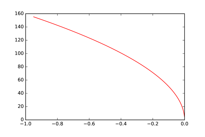
Figure 3. The dependence of the $z$-axis equilibrium point distance on the $C_{20}$ rescaled, see (3.14).

To convert to real units, the distances from the equilibrium points to the center need to be multiplied by $m_{3}^{1/3}$ – due to the rescaling involved in the Hill procedure –, and by the unit of distance which in this case is the distance Sun-Jupiter. It follows that the $x$-axis equilibrium points are at a distance of $85,512.774$ km from Hektor, the $x$-axis equilibrium points are at a distance of $956,149.406$ km, and the $z$-axis equilibrium points are at a distance of $110.028$ km. As the smallest semi-minor axis of Hektor is $60$ km, the $z$-axis equilibrium points are outside the body of the asteroid. It seems though that for many other asteroids the $z$-axis equilibrium points are located inside their body.

Remark 4.1.

These $z$-axis equilibria also appear in the case of the motion of a particle in a geopotential field (see, e.g., [CG14]). From that model it can be derived that the distance from the $z$-axis equilibrium points to the center is given by $\hat{r}_{z}=R_{3}(-3C_{20})^{1/2}$. When we apply this formula in the case of Hektor, the numerical result is very close to the one found above. This formula can be derived from the equation $h_{C}(r)=0$ if we drop the term $r^{5}$.

4.2. Linear stability of the equilibrium points

We study the linear stability of the equilibrium points in the case of Hektor.

The Hamiltonian (3.15) yields the following system of equations

$$\dot{x}=v_{x}, \dot{v}_{x}=2v_{y}+\Omega_{x},$$

$$\dot{y}=v_{y}, \dot{v}_{y}=-v_{x}+\Omega_{y},$$

$$\dot{z}=v_{z}, \dot{v}_{z}=\Omega_{z},$$

where $\Omega$ is the effective potential given by (3.18) (again, we omit the overline bar on the variables).

The second order derivatives of $\Omega$ are given by

(4.2) $$\begin{split}\Omega_{xx}=&\lambda_{2}-\frac{1}{r^{3}}+\frac{3x^{2}}{r^{5}}+\frac{3c}{r^{5}}-\frac{15cx^{2}}{r^{7}}-\frac{15cz^{2}}{r^{7}}+\frac{105cz^{2}x^{2}}{r^{9}},\\ \Omega_{yy}=&\lambda_{1}-\frac{1}{r^{3}}+\frac{3y^{2}}{r^{5}}+\frac{3c}{r^{5}}-\frac{15cy^{2}}{r^{7}}-\frac{15cz^{2}}{r^{7}}+\frac{105cz^{2}y^{2}}{r^{9}},\\ \Omega_{zz}=&-1-\frac{1}{r^{3}}+\frac{3z^{2}}{r^{5}}+\frac{9c}{r^{5}}-\frac{90cz^{2}}{r^{7}}+\frac{105cz^{4}}{r^{9}},\\ \Omega_{xy}=&\frac{3xy}{r^{5}}-\frac{15cxy}{r^{7}}+\frac{105cz^{2}xy}{r^{9}},\\ \Omega_{xz}=&\frac{3xz}{r^{5}}-\frac{45cxz}{r^{7}}+\frac{105cz^{3}x}{r^{9}},\\ \Omega_{yz}=&\frac{3yz}{r^{5}}-\frac{45cyz}{r^{7}}+\frac{105cz^{3}y}{r^{9}}.\end{split}$$

The Jacobian matrix describing the linearized system is

(4.3) $$\mathscr{J}=\left(\begin{array}[]{rrrrrr}0&0&0&1&0&0\\ 0&0&0&0&1&0\\ 0&0&0&0&0&1\\ \Omega_{xx}&\Omega_{xy}&\Omega_{xz}&0&2&0\\ \Omega_{yx}&\Omega_{yy}&\Omega_{yz}&-2&0&0\\ \Omega_{zx}&\Omega_{zy}&\Omega_{zz}&0&0&0\\ \end{array}\right).$$

Since the equilibria are of the form $(\pm r^{*}_{x},0,0)$, $(0,\pm r^{*}_{y},0)$, $(0,0,\pm r^{*}_{z})$, the mixed second order partial derivatives $\Omega_{xy}$, $\Omega_{xz}$, $\Omega_{yz}$ vanish at each of the equilibrium points.

Hence Jacobian matrix (4.3) evaluated at the equilibria is of the form:

(4.4) $$\mathscr{J}=\left(\begin{array}[]{rrrrrr}0&0&0&1&0&0\\ 0&0&0&0&1&0\\ 0&0&0&0&0&1\\ \Omega_{xx}&0&0&0&2&0\\ 0&\Omega_{yy}&0&-2&0&0\\ 0&0&\Omega_{zz}&0&0&0\\ \end{array}\right),$$

The characteristic equation of (4.4) is

(4.5) $$(\rho^{2}-\Omega_{zz})(\rho^{4}+(4-\Omega_{xx}-\Omega_{yy})\rho^{2}+\Omega_{xx}\Omega_{yy})=0.$$

The stability of the equilibria depends on the signs of $\Omega_{zz}$ and of $A$, $B$, and $D$.

We find the following stability character of the equilibrium positions in the case of the Sun-Jupiter-Hektor system:

$i)$ Eigenvalues of $x$-axis equilibria at $(\pm 0.6935267570,0,0)$:

$$2.50694248 -2.50694248,$$

$$2.07048307i, -2.07048307i,$$

$$1.99946504i, -1.99946504i.$$

Stability type: center $\times$ center $\times$ saddle.

$ii)$ Eigenvalues of $y$-axis equilibria at $(0,7.7545747196,0)$:

$$0.98901573i, -0.98901573i,$$

$$0.14036874i, -0.14036874i,$$

$$1.00107168i, -1.00107168i$$

Stability type: center $\times$ center $\times$ center.

$iii)$ Eigenvalues of $z$-axis equilibria at $(0,0,\pm 0.0008923544)$:

$$37514.0432165187+0.9999999998i, -37514.0432165187+0.9999999998j,$$

$$37514.0432165187-0.9999999998i, -37514.0432165187-0.9999999998i$$

$$53052.8687i, -53052.8687i$$

Stability type: center $\times$ complex saddle.

Note that for the $z$-axis equilibria the imaginary part of the ‘Krein quartet’ of eigenvalues of $z$-axis equilibria is approximately $\pm 1$. This means that the infinitesimal motion around the equilibrium point is close to the $1:1$ resonance with the rotation of the primary and the secondary. In Fig. 4 we show that for a range of $r^{*}_{z}$ values between $z=0.000892354498497342$ (corresponding to the $c$ value for Hektor) and $z=0.01$ (corresponding to $c=-1.666668333\times 10^{-5}$), the real part and the imaginary part of the ‘Krein quartet’ of eigenvalues; the imaginary part stays close to $\pm 1$.

$\begin{array}[]{cc}\includegraphics[width=216.81pt]{real_part_eigenvalues}&\includegraphics[width=216.81pt]{imaginary_part_eigenvalues}\end{array}$

Figure 4. The dependence of the real part (left) and imaginary part (right) of the Krein quartet of eigenvalues on the $z$-axis equilibrium point. The horizontal axis represents the distance $r^{*}_{z}$ from the equilibrium point to the origin, the vertical axis the real part (left), and the absolute value of the imaginary part (right) of the eigenvalues. The former never changes sign, and the latter stays within $4\times 10^{-7}$ from $1$.

In Section 4.2.1 we will provide an analytic argument that the real part of the ‘Krein quartet’ of eigenvalues is always non-zero, and the imaginary part is close to $\pm 1$ for $r^{*}_{z}$ sufficiently small; this result will help us to explain the behavior observed in Fig. 4.

In the sequel we give a more detailed analysis of the linear stability of all equilibria, for a wide range of parameters $\mu$ and $c$.

4.2.1. Linear stability of the equilibria on the $z$-axis

The $z$-axis equilibrium points are of the form $(0,0,\pm r^{*}_{z})$, with

(4.6) $$-(r^{*}_{z})^{5}-(r^{*}_{z})^{2}-6c=0,$$

which yields

(4.7) $$c=\frac{-(r^{*}_{z})^{2}-(r^{*}_{z})^{5}}{6}.$$

Evaluating $\Omega_{xx}$, $\Omega_{yy}$, $\Omega_{zz}$ at the equilibrium point yields:

$$\begin{split}\Omega_{xx}=&\lambda_{2}-(r^{*}_{z})^{-3}-12c(r^{*}_{z})^{-5},\\ \Omega_{yy}=&\lambda_{1}-(r^{*}_{z})^{-3}-12c(r^{*}_{z})^{-5},\\ \Omega_{zz}=&-1+2(r^{*}_{z})^{-3}+24c(r^{*}_{z})^{-5}.\end{split}$$

Substituting in (4.7) we have

(4.8) $$\begin{split}\Omega_{xx}&=2+\lambda_{2}+(r^{*}_{z})^{-3},\\ \Omega_{yy}&=2+\lambda_{1}+(r^{*}_{z})^{-3},\\ \Omega_{zz}&=-5-2(r^{*}_{z})^{-3}.\end{split}$$

Using (3.16) and denoting $d:=\sqrt{1-v^{2}(4-v^{2})(\mu-\mu^{2})}$ we can write

(4.9) $$\begin{split}\lambda_{1}=\frac{3}{2}(1-d),\\ \lambda_{2}=\frac{3}{2}(1+d).\end{split}$$

Also for $c=0$ we have $d_{0}=\sqrt{1-3(\mu-\mu^{2})}$ and

(4.10) $$\begin{split}\lambda_{10}=&\frac{3}{2}(1-d_{0}),\\ \lambda_{20}=&\frac{3}{2}(1+d_{0}).\end{split}$$

This is in agreement with the results in [BGG15].

For future reference, we expand $d$ as a power series in the parameter $c$ as

(4.11) $$d=d_{0}+d_{1}c+O(c^{2}),$$

where the coefficient $d_{1}$ can be obtained can be obtained from the Taylor’s theorem around $c=0$ as

(4.12) $$\begin{split}d_{1}=&-\frac{2(\mu-\mu^{2})}{d_{0}}m_{3}^{2/3}.\end{split}$$

From the characteristic equation (4.5), we obtain that the pair of eigenvalues $\rho_{1,2}=\pm(\Omega_{zz})^{1/2}$ is purely imaginary, since by (4.8), $\Omega_{zz}<0$.

The ‘Krein quartet’ eigenvalues are given by

(4.13) $$\rho_{3,4,5,6}=\pm\sqrt{\frac{-A\pm\sqrt{A^{2}-4B}}{2}},$$

where

$$\begin{array}[]{lllll}A&=&\displaystyle 4-\Omega_{xx}-\Omega_{yy}&=&-3-\frac{2}{(r^{*}_{z})^{3}},\\ B&=&\Omega_{xx}\Omega_{yy}&=&\displaystyle 10+{9\over 4}v^{2}(4-v^{2})(\mu-\mu^{2})+\frac{7}{(r^{*}_{z})^{3}}+\frac{1}{(r^{*}_{z})^{6}}.\end{array}$$

Then we have

$$\begin{split}D:=A^{2}-4B=&d^{2}-40-\frac{16}{(r^{*}_{z})^{3}}=-31-9v^{2}(4-v^{2})(\mu-\mu^{2})-\frac{16}{(r^{*}_{z})^{3}}<0.\end{split}$$

Since $-A>0$ and $D<0$, we obtain that the eigenvalues $\rho_{3,4,5,6}$ are complex numbers, non-real, non-purely-imaginary, for all parameter values. Let $\rho=a+ib$ be such that $\rho^{2}=-\frac{A}{2}\pm\frac{\sqrt{4B-A^{2}}}{2}i:=\alpha+i\beta$. We have

$$a+ib=\left(\frac{(\alpha^{2}+\beta^{2})^{\frac{1}{2}}+\alpha}{2}\right)^{\frac{1}{2}}+\textrm{sign}(\beta)\left(\frac{(\alpha^{2}+\beta^{2})^{\frac{1}{2}}-\alpha}{2}\right)^{\frac{1}{2}}\ i.$$

To show that $b$ is approximately $\pm 1$, or $b^{2}\approx 1$, for $r^{*}_{z}\approx 0$, note that

$$\begin{split}b^{2}=&\frac{(\alpha^{2}+\beta^{2})^{\frac{1}{2}}-\alpha}{2}=\frac{A}{4}+\frac{\sqrt{B}}{2}\\ =&-\frac{3}{4}+\frac{1}{2}\left[\left(10+\frac{9}{4}\Upsilon+\frac{7}{(r^{*}_{z})^{3}}+\frac{1}{(r^{*}_{z})^{6}}\right)^{\frac{1}{2}}-\frac{1}{(r^{*}_{z})^{3}}\right]\\ =&-\frac{3}{4}+\frac{1}{2}\frac{10+\frac{9}{4}\Upsilon+\frac{7}{(r^{*}_{z})^{3}}+\frac{1}{(r^{*}_{z})^{6}}-\frac{1}{(r^{*}_{z})^{6}}}{\left(10+\frac{9}{4}\Upsilon+\frac{7}{(r^{*}_{z})^{3}}+\frac{1}{(r^{*}_{z})^{6}}\right)^{\frac{1}{2}}+\frac{1}{(r^{*}_{z})^{3}}}\\ =&-\frac{3}{4}+\frac{1}{2}\frac{10+\frac{9}{4}\Upsilon+\frac{7}{(r^{*}_{z})^{3}}}{\left(10+\frac{9}{4}\Upsilon+\frac{7}{(r^{*}_{z})^{3}}+\frac{1}{(r^{*}_{z})^{6}}\right)^{\frac{1}{2}}+\frac{1}{(r^{*}_{z})^{3}}},\end{split}$$

where $\Upsilon:=v^{2}(4-v^{2})(\mu-\mu^{2})$. Since

$$\lim_{r^{*}_{z}\to 0}\frac{10+\frac{9}{4}\Upsilon+\frac{7}{(r^{*}_{z})^{3}}}{\left(10+\frac{9}{4}\Upsilon+\frac{7}{(r^{*}_{z})^{3}}+\frac{1}{(r^{*}_{z})^{6}}\right)^{\frac{1}{2}}+\frac{1}{(r^{*}_{z})^{3}}}=\frac{7}{2},$$

we have that $\lim_{r^{*}_{z}\to 0}b^{2}=-\frac{3}{4}+\frac{7}{4}=1$, so $b^{2}\approx 1$ for $r^{*}_{z}\approx 0$, as in the case of Hektor.

We obtained the following result:

Proposition 4.2.

Consider the equilibria on the $z$-axis. For $\mu\in(0,1/2]$, $\Omega_{zz}$, $A$ and $D$ are negative. Consequently, one pair of eigenvalues is purely imaginary, and the two other pairs of eigenvalues are complex conjugate, with the imaginary part close to $\pm i$ for $c$ negative and sufficiently small. The linear stability is of center $\times$ complex-saddle type.

4.2.2. Linear stability of the equilibria on the $y$-axis

The $y$-axis equilibrium points are of the form $(0,\pm r^{*}_{y},0)$, with

(4.14) $$\lambda_{1}(r^{*}_{y})^{5}-(r^{*}_{y})^{2}+3c=0,$$

which yields

(4.15) $$c=\frac{(r^{*}_{y})^{2}-\lambda_{1}(r^{*}_{y})^{5}}{3}.$$

Evaluating $\Omega_{xx}$, $\Omega_{yy}$, $\Omega_{zz}$ at the equilibrium point yields:

(4.16) $$\begin{split}\Omega_{xx}=&\lambda_{2}-\frac{1}{(r^{*}_{y})^{3}}+\frac{3c}{(r^{*}_{y})^{5}},\\ \Omega_{yy}=&\lambda_{1}+\frac{2}{(r^{*}_{y})^{3}}-\frac{12c}{(r^{*}_{y})^{5}},\\ \Omega_{zz}=&-1-\frac{1}{(r^{*}_{y})^{3}}+\frac{9c}{(r^{*}_{y})^{5}}.\end{split}$$

Substituting $c$ from (4.15) we obtain

(4.17) $$\begin{split}\Omega_{xx}=&\lambda_{2}-\lambda_{1},\\ \Omega_{yy}=&5\lambda_{1}-\frac{2}{(r^{*}_{y})^{3}},\\ \Omega_{zz}=&-1-3\lambda_{1}+\frac{2}{(r^{*}_{y})^{3}},\end{split}$$

We also expand $r^{*}_{y}$ as a power series in the parameter $c$ as

(4.18) $$r^{*}_{y}=r_{y0}+r_{y1}c+O(c^{2}),$$

where $\pm r_{y0}$ is the position of the $y$-equilibrium in the case when $c=0$, which is given by $r_{y0}^{3}=1/\lambda_{10}$; this is in agreement with [BGG15]. The computation of $r_{y1}$ yields

(4.19) $$\begin{split}r_{y1}=&\frac{-1+(1/2)d_{1}r_{y0}^{5}}{r_{y0}},\end{split}$$

with $d_{1}$ as in (4.12).

We will also need $\frac{1}{(r^{*}_{y})^{3}}$ as a power series in the parameter $c$

(4.20) $$\frac{1}{(r^{*}_{y})^{3}}=\alpha+\beta c+O(c^{2}),$$

and a simple calculation yields

(4.21) $$\begin{split}\alpha=&\frac{1}{r_{y0}^{3}},\\ \beta=&-\frac{3r_{y1}}{r_{y0}^{4}}.\end{split}$$

For $\mu=1/2$, we have $d_{0}=\frac{1}{2}$, $\lambda_{10}=\frac{3}{4}$, $d_{1}=-m_{3}^{2/3}$, $r_{y0}=\left(\frac{4}{3}\right)^{1/3}$. It is easy to see that dominant part $d_{0}$ of $d$ is a strictly decreasing function with respect to $\mu\in(0,1/2]$ and takes values in $[1/2,1)$. The dominant part $\lambda_{10}$ of $\lambda_{1}$ is increasing with respect to $\mu\in(0,1/2]$ and takes values in $(0,3/4]$. Also, the dominant part $r_{y0}$ of $r^{*}_{y}$ is a strictly decreasing function in $\mu\in(0,1/2]$, where $r_{y0}(1/2)=\sqrt[3]{4/3}$ and $r_{y0}\rightarrow\infty$ when $\mu\rightarrow 0$; as a consequence the values of $r_{y0}$ are in the interval $[\sqrt[3]{4/3},\infty)$.

From (4.16) we have

$$\begin{split}\Omega_{zz}&=-1-\frac{1}{(r^{*}_{y})^{3}}+\frac{9c}{(r^{*}_{y})^{5}}\\ &=-\frac{1}{(r^{*}_{y})^{5}}((r^{*}_{y})^{5}+(r^{*}_{y})^{2}-9c)\\ &<0\end{split}$$

since $r^{*}_{y}>0$ and $c$ is negative. Therefore, $\Omega_{zz}<0$ for all admissible values of $\mu$.

For $A=4-\Omega_{xx}-\Omega_{yy}$, using (4.10) and the expansions (4.11) and (4.20) we obtain

$$\begin{split}A&=1-3\lambda_{1}+\frac{2}{(r^{*}_{y})^{3}}\\ &=1-3\lambda_{10}+\frac{2}{(r_{y0})^{3}}+O(c)\\ &=1-3\lambda_{10}+2\lambda_{10}+O(c)\\ &>0\end{split}$$

for $c$ small.

For $B=\Omega_{xx}\Omega_{yy}$ using (4.10) and the expansions (4.11) and (4.20) we obtain

$$\begin{split}B&=(\lambda_{2}-\lambda_{1})\left(5\lambda_{1}-\frac{2}{(r^{*}_{y})^{3}}\right)\\ &=(3d)\left(\frac{15}{2}-\frac{15d}{2}-\frac{2}{(r^{*}_{y})^{3}}\right)\\ &=(3d_{0})\left(5\lambda_{10}-\frac{2}{r_{y0}^{3}}\right)+O(c)\\ &=(3d_{0})\left(5\lambda_{10}-2\lambda_{10}\right)+O(c)\\ &>0\end{split}$$

for $c$ small.

For $D=A^{2}-4B$, using (4.10) and the expansions (4.11) and (4.20) we have

$$\begin{split}D&=\left(1-3\lambda_{10}+\frac{2}{r_{y0}^{3}}\right)^{2}-4(3d_{0})\left(5\lambda_{10}-\frac{2}{r_{y0}^{3}}\right)+O(c)\\ &=\left(1-\lambda_{10}\right)^{2}-12(3-2\lambda_{10})\lambda_{10}+O(c).\end{split}$$

For $\mu\approx 0$ we have $D\approx 1+O(c)$ and for $\mu=1/2$ we have $D=-\frac{215}{16}+O(c)$. The intermediate value theorem implies that $D$ changes its sign from positive to negative for $\mu\in(0,1/2]$, provided $c$ is small. We have thus proved the following result:

Proposition 4.3.

Consider the equilibria on the $y$-axis. For $\mu\in(0,1/2]$ and for the parameter $c$ negative and small enough, $\Omega_{zz}$ is always negative, the coefficients $A$ and $B$ are always positive, and the value of the discriminant $D$ changes from positive to negative values. Consequently, one pair of eigenvalues is always purely imaginary, and there exists $\mu_{*}$, depending on $c_{20}$, where the other two pairs of eigenvalues change from being purely imaginary to being complex conjugate. The linear stability changes from center $\times$ center $\times$ center type to center $\times$ complex-saddle type.

4.2.3. Linear stability of the equilibria on the $x$-axis

The $x$-axis equilibrium points are of the form $(\pm r^{*}_{x},0,0)$, with

(4.22) $$\lambda_{2}(r^{*}_{x})^{5}-(r^{*}_{x})^{2}+3c=0,$$

which yields

(4.23) $$c=\frac{(r^{*}_{x})^{2}-\lambda_{2}(r^{*}_{x})^{5}}{3}.$$

Evaluating $\Omega_{xx}$, $\Omega_{yy}$, $\Omega_{zz}$ at the equilibrium point yields:

(4.24) $$\begin{split}\Omega_{xx}=&\lambda_{2}+\frac{2}{(r^{*}_{x})^{3}}-\frac{12c}{(r^{*}_{x})^{5}},\\ \Omega_{yy}=&\lambda_{1}-\frac{1}{(r^{*}_{x})^{3}}+\frac{3c}{(r^{*}_{x})^{5}},\\ \Omega_{zz}=&-1-\frac{1}{(r^{*}_{x})^{3}}+\frac{9c}{(r^{*}_{x})^{5}}.\end{split}$$

Substituting $c$ from (4.23) we obtain

(4.25) $$\begin{split}\Omega_{xx}=&5\lambda_{2}-\frac{2}{(r^{*}_{x})^{3}},\\ \Omega_{yy}=&\lambda_{1}-\lambda_{2},\\ \Omega_{zz}=&-1-3\lambda_{2}+\frac{2}{(r^{*}_{x})^{3}},\end{split}$$

We expand $r^{*}_{x}$ as a power series in the parameter $c$ as

(4.26) $$r^{*}_{x}=r_{x0}+r_{x1}c+O(c^{2}),$$

where $\pm r_{x0}$ is the position of the $x$-equilibrium in the case when $c=0$, which is given by $r_{x0}^{3}=1/\lambda_{20}$; see [BGG15]. The computation of $r_{x1}$ yields

(4.27) $$\begin{split}r_{x1}=&\frac{-1-(1/2)d_{1}r_{x0}^{5}}{r_{x0}}.\end{split}$$

We will also need $\frac{1}{(r^{*}_{x})^{3}}$ as a power series in the parameter $c$

(4.28) $$\frac{1}{(r^{*}_{x})^{3}}=\alpha^{\prime}+\beta^{\prime}c+O(c^{2}),$$

and a simple calculation yields

(4.29) $$\begin{split}\alpha^{\prime}=&\frac{1}{r_{x0}^{3}},\\ \beta^{\prime}=&-\frac{3r_{x1}}{r_{x0}^{4}}.\end{split}$$

From (4.24) we have

$$\begin{split}\Omega_{zz}&=-1-\frac{1}{(r^{*}_{x})^{3}}+\frac{9c}{(r^{*}_{x})^{5}}\\ &=-\frac{1}{(r^{*}_{x})^{5}}((r^{*}_{x})^{5}+(r^{*}_{x})^{2}-9c)\\ &<0\end{split}$$

since $r^{*}_{x}>0$ and $c<0$. Therefore, $\Omega_{zz}<0$ for all admissible values of $\mu$.

For $A=4-\Omega_{xx}-\Omega_{yy}$, using (4.10) and the expansions (4.11) and (4.28), we obtain

$$\begin{split}A&=1-3\lambda_{20}+\frac{2}{(r_{x0})^{3}}+O(c)\\ &=1-\lambda_{20}+O(c)\\ &=-\frac{1}{2}-\frac{3}{2}d_{0}+O(c)\\ &<0\end{split}$$

for $c$ small.

For $B=\Omega_{xx}\Omega_{yy}$, using (4.10) and the expansions (4.11) and (4.28). we obtain

$$\begin{split}B&=-(3d_{0})\left(5\lambda_{20}-\frac{2}{r_{x0}^{3}}\right)+O(c)\\ &=-(3d_{0})\left(5\lambda_{20}-2\lambda_{20}\right)+O(c)\\ &=-9d_{0}\left(\frac{3}{2}+\frac{3}{2}d_{0}\right)\\ &<0\end{split}$$

for $c$ small.

For $D=A^{2}-4B$, using (4.10) and the expansions (4.11) and (4.28) we have

$$\begin{split}D&=\left(1-\lambda_{20}\right)^{2}+36d_{0}\lambda_{20}+O(c)\\ &>0.\end{split}$$

for $c$ small.

We have proved the following result:

Proposition 4.4.

Consider the equilibria on the $x$-axis. For $\mu\in(0,1/2]$ and for parameter $c$ negative and small enough, $\Omega_{zz}$ is negative, $A$ and $B$ are negative, and the value of the discriminant $D$ is always positive. Consequently, two pairs of eigenvalues are purely imaginary, and one pair of eigenvalues are real (one positive and one negative). The linear stability is of center $\times$ center $\times$ saddle type.

References

• [AGST12] John A Arredondo, Jianguang Guo, Cristina Stoica, and Claudia Tamayo. On the restricted three body problem with oblate primaries. Astrophysics and Space Science, 341(2):315–322, 2012.
• [APC13] John Alexander Arredondo and Ernesto Perez-Chavela. Central configurations in the Schwarzschild three body problem. Qualitative theory of dynamical systems, 12(1):183–206, 2013.
• [APHS16] Md Chand Asique, Umakant Prasad, M. R. Hassan, and Md Sanam Suraj. On the photogravitational R4BP when the third primary is a triaxial rigid body. Astrophysics and Space Science, 361(12):379, Nov 2016.
• [ARV09] Martha Alvarez-Ramirez and Claudio Vidal. Dynamical aspects of an equilateral restricted four-body problem. Mathematical Problems in Engineering, 2009:Article ID 181360, 23 p., 2009.
• [BG16] J. Burgos-García. Families of periodic orbits in the planar Hill’s four-body problem. ArXiv e-prints, 361:353, November 2016.
• [BGD13a] Jaime Burgos-García and Joaquín Delgado. On the “blue sky catastrophe” termination in the restricted four-body problem. Celestial Mechanics and Dynamical Astronomy, 117(2):113–136, 2013.
• [BGD13b] Jaime Burgos-García and Joaquín Delgado. Periodic orbits in the restricted four-body problem with two equal masses. Astrophysics and Space Science, 345(2):247–263, 2013.
• [BGG15] Jaime Burgos-García and Marian Gidea. Hill’s approximation in a restricted four-body problem. Celestial Mechanics and Dynamical Astronomy, 122(2):117–141, 2015.
• [Boy97] W. Boyce. Comment on a formula for the gravitational harmonic coefficients of a triaxial ellipsoid. Celestial Mechanics and Dynamical Astronomy, 67:107–110, February 1997.
• [BP13] A.N. Baltagiannis and K.E. Papadakis. Periodic solutions in the Sun–Jupiter–Trojan asteroid–Spacecraft system. Planetary and Space Science, 75:148–157, 2013.
• [CG14] Alessandra Celletti and Cătălin Galeş. On the dynamics of space debris: 1: 1 and 2: 1 resonances. Journal of Nonlinear Science, 24(6):1231–1262, 2014.
• [CG18] Alessandra Celletti and Catalin Gales. Dynamics of resonances and equilibria of Low Earth Objects. SIAM Journal on Applied Dynamical Systems, 17(1):203–235, 2018.
• [CLPC04] Montserrat Corbera, Jaume Llibre, and Ernesto Pérez-Chavela. Equilibrium points and central configurations for the Lennard-Jones 2- and 3-body problems. Celestial Mechanics and Dynamical Astronomy, 89(3):235–266, Apr 2004.
• [Del11] Nicolas Delsate. Analytical and numerical study of the ground-track resonances of Dawn orbiting Vesta. Planetary and Space Science, 59(13):1372–1383, 2011.
• [Des15] Pascal Descamps. Dumb-bell-shaped equilibrium figures for fiducial contact-binary asteroids and EKBOs. Icarus, 245:64 – 79, 2015.
• [DLZ12] R. Dvorak, C. Lhotka, and L. Zhou. The orbit of 2010 TK7: possible regions of stability for other Earth Trojan asteroids. Astronomy $\&$ Astrophysics, 541:A127, 2012.
• [DSZ] Florin Diacu, Cristina Stoica, and Shuqiang Zhu. Central configurations of the curved n-body problem. Journal of Nonlinear Science, pages 1–48.
• [GJ03] Frederic Gabern and Angel Jorba. Restricted four and five body problems in the solar system. In Libration Point Orbits And Applications, pages 573–586. World Scientific, 2003.
• [GN12] Marian Gidea and Constantin P Niculescu. A Brief Account on Lagrange’s Algebraic Identity. The Mathematical Intelligencer, 34(3):55–61, 2012.
• [Hil78] G. W. Hill. Researches in the lunar theory. American Journal of Mathematics, 1(1):5–26, 1878.
• [HS86] K.C. Howell and D.B. Spencer. Periodic orbits in the restricted four-body problem. Acta Astronautica, 13(8):473 – 479, 1986.
• [JPL] JPL Solar System Dynamics. https://ssd.jpl.nasa.gov/. Accessed: 2018-08-01.
• [KMJ17] S. Kepley and J. D. Mireles James. Chaotic motions in the restricted four body problem via Devaney’s saddle-focus homoclinic tangle theorem. ArXiv e-prints, November 2017.
• [LC15] C. Lhotka and A. Celletti. The effect of Poynting-Robertson drag on the triangular Lagrangian points. Icarus, 250:249–261, 2015.
• [McC63] S.W. McCuskey. Introduction to celestial mechanics. Addison-Wesley Series in Aerospace Science. Addison-Wesley, 1963.
• [MDCR+14] F. Marchis, J. Durech, J. Castillo-Rogez, F. Vachier, M. Cuk, J. Berthier, M.H. Wong, P. Kalas, G. Duchene, M.A. Van Dam, et al. The puzzling mutual orbit of the binary Trojan asteroid (624) Hektor. The Astrophysical journal letters, 783(2):L37, 2014.
• [MRPD01] V. V. Markellos, A. E. Roy, E. A. Perdios, and C. N. Douskos. A Hill problem with oblate primaries and effect of oblateness on Hill stability of orbits. Astrophysics and Space Science, 278:295–304, 2001.
• [MS82] Kenneth R. Meyer and Dieter S. Schmidt. Hill’s lunar equations and the three-body problem. Journal of Differential Equations, 44(2):263 – 272, 1982.
• [MS17] Regina Martínez and Carles Simó. Relative equilibria of the restricted three-body problem in curved spaces. Celestial Mechanics and Dynamical Astronomy, 128(2):221–259, Jun 2017.
• [SB05] Daniel Jay Scheeres and Julie Bellerose. The restricted Hill full 4-body problem: application to spacecraft motion about binary asteroids. Dynamical Systems, 20(1):23–44, 2005.
• [Sch98] DJ Scheeres. The restricted Hill four-body problem with applications to the Earth–Moon–Sun system. Celestial Mechanics and Dynamical Astronomy, 70(2):75–98, 1998.
• [SR76] Ram Krishan Sharma and PV Subba Rao. Stationary solutions and their characteristic exponents in the restricted three-body problem when the more massive primary is an oblate spheroid. Celestial Mechanics, 13(2):137–149, 1976.