A re-examination of the role of friction in the original Social Force Model

Abstract

The fundamental diagram of pedestrian dynamics gives the relation between the density and the flow within a specific enclosure. It is characterized by two distinctive behaviors: the free-flow regime (for low densities) and the congested regime (for high densities). In the former, the flow is an increasing function of the density, while in the latter, the flow remains on hold or decreases. In this work, we perform numerical simulations of the pilgrimage at the entrance of the Jamaraat bridge (pedestrians walking along a straight corridor) and compare flow-density measurements with empirical measurements made by Helbing et al [1]. We show that under high density conditions, the basic Social Force Model (SFM) does not completely handle the fundamental diagram reported in empirical measurements. We use analytical techniques and numerical simulations to prove that with an appropriate modification of the friction coefficient (but sustaining the SFM) it is possible to attain behaviors which are in qualitative agreement with the empirical data. Other authors have already proposed a modification of the relaxation time in order to address this problem. In this work, we unveil the fact that our approach is analogous to theirs since both affect the same term of the reduced-in-units equation of motion. We show how the friction modification affects the pedestrian clustering structures throughout the transition from the free-flow regime to the congested regime. We also show that the speed profile, normalized by width and maximum velocity yields a universal behavior regardless of the corridor dimensions.

1 Introduction

In the last decades, many microscopic models for crowd dynamics were developed. Force-based models were introduced by Hirai and Tarui [2] who in 1975 proposed to associate the interaction between pedestrians and their environment using different kinds of forces inspired by physical systems. For example, Okazaki (1979) modeled the movement of pedestrians as a magnetized object immersed a magnetic in field [3].

By the late 90’s and the beginning of the century, Helbing et al. proposed a model that included socio-psychological and physical forces to simulate crowd dynamics. According to Helbing et al., both the environment and the individuals’ own desire affect the pedestrians motion in a similar way as forces do with respect to the momentum of particles [4, 5]. This “Social Force Model” (SFM) related the socio-psychological phenomenon of crowds behavior to the “microscopic” formalism of moving particles. The model succeeded in reproducing the reduction of the efficiency of the evacuation process as pedestrians try harder to escape from a dangerous situation (i.e. “faster is slower” effect) [4, 6]. The faster-is-slower effect was well explained as a consequence of the presence of human blocking clusters that obstruct the exit during an emergency evacuation [7].

The SFM, in its basic version, was reported to be suitable for describing, at least qualitatively, a variety of emergency situations, including the presence of obstacles, or the existence of more than one exit [8, 9]. Scenarios described in Refs. [10, 11, 12] required, however, a step up implementation although sustaining the basic model and its parameters.

In the last years, several extensions of the SFM have been proposed. These extensions solve numerical pitfalls [13] and other issues such as oscillations, overlapping and non-realistic trajectories [14, 15]. However, many of these extensions do not correspond to the assumptions that motivated the original SFM [4, 5], focusing on the individual behavior of each agent. The basic SFM assumes strong interactions in a dense environment.

Some questioning arose on the true psychological tendency of the pedestrians to stay away from each other. While the social forces accomplish this tendency, it attains a somewhat unrealistic “colliding behavior” for slowly moving pedestrians [16]. His (her) repulsive tendency is expected to decrease as approaching a more crowded environment. The small fall-off length $B=0.08\,$m suggested by Helbing in Ref. [4] does not completely solve this issue. It neither agrees with the fact that pedestrians prefer to keep a comfortable $0.5\,$m distance between each other in a moderately crowded environment, nor it fits accurately the empirical velocities reported for crowds under normal conditions [16].

Researchers turned back to examine the available data on the velocity and flux behavior for different density environments [17, 1, 18, 19]. Ref. [1] summarizes empirical data from the literature, and their own data set, acquired from videos of the Muslim pilgrimage in Mina-Makkah (2006). They showed from the empirical fundamental diagram (flux $J$ versus density $\rho$) that highly dense crowds (seemingly up to $10\,$p m^-2) do not drive the pedestrians velocity to zero, although the reasons for this remain rather obscure.

More recent findings on the fundamental diagram for an extremely dense situation show that, sometimes, the flux may increase with the density (see Ref. [20]). This seems to contradict the results of Ref. [1]. But both results appear not to be completely comparable since data was acquired at different points, and thus, at different stages of the ritual. Ref. [20], indeed, states that the fundamental diagram may strongly depend on the type of motion and the nature of the event.

Our work focuses on data from Ref. [1]. Further measurements can be found in Refs. [17, 20, 21, 22, 23]. The PedFlow model developed by Löhner et al. (Ref. [24]) is an alternative to the Helbing model. Togashi et al. improved the calibration of this model using a Kalman filter ensemble [25].

The high density regime appears to be the most complicated one. Caution was claimed when (automatically) transferring the usual “calibrated” parameters of the SFM to this regime. It was argued that the pedestrians’ body size distribution and the “situational context” are somewhat responsible for the unexpected departure from the original SFM parameters [26, 27]. But other researchers pointed out that this departure actually expresses the lack of a mechanism to properly handle the pedestrians’ “required space to move”. Some modifications to the basic SFM were then proposed to overcome this difficulty [28, 29].

A mechanism allowing an “increase of the space to move” (particularly in relaxed/low density situations) is a compelling necessity in the context of the SFM. But a sharp “re-calibration” of the model for high density situations appears not to be completely satisfactory [30]. A more “natural” way of handling this matter requires a deep examination of the current SFM parameters. The net-time headway (roughly, the relaxation time) was first examined in Ref. [30]. The author sustains the hypothesis that the pedestrians net-time headway should increase until there is “enough space to make a step”. He shows that a density dependent net-time headway is a suitable parameter to smartly reproduce the empirical fundamental diagram for highly dense crowds [30].

Our own examination of the SFM parameters suggests that not only the net-time headway, but the friction between pedestrians (and with the walls) can reproduce the pattern of the fundamental diagram. Our working hypothesis is that friction is the crucial parameter in the dynamics of highly dense crowds. We actually sustain the SFM model with no further “re-calibrations”, but with the right friction value, in order to meet the fundamental diagram pattern.

We want to emphasize that although the friction value appearing in Ref. [4] is a commonly accepted estimate throughout the literature, other values have also been proposed [31]. We propose our value as an experimentally based parameter, suitable for highly dense crowds.

The investigation is organized as follows. We first recall the SFM in Section 2.1, while including the precise definitions for flux, density and clustered structures. Section 3 presents our numerical simulations for pedestrians moving along corridors. The hypotheses of the work are stated in Section 4. The corresponding results are shown in Section 5. Our main conclusions are detailed in Section 6.

2 Background

2.1 The Social Force Model

Our research was carried out in the context of the “Social Force Model” (SFM) proposed by Helbing et al. [4]. This model states that human motion is caused by the desire of people to reach a certain destination at a certain velocity, as well as other environmental factors. The pedestrians’ behavioral pattern in a crowded environment can be modeled by three kinds of forces: the “desire force”, the “social force” and the “granular force”.

The “desire force” represents the pedestrian’s own desire to reach a specific target position at a desired velocity $v_{d}$. But, in order to reach the desired target, he (she) needs to accelerate (decelerate) from his (her) current velocity $\mathbf{v}^{(i)}(t)$. This acceleration (or deceleration) represents a “desire force” since it is motivated by his (her) own willingness. The corresponding expression for this forces is

$$\mathbf{f}_{d}^{(i)}(t)=m_{i}\,\displaystyle\frac{v_{d}^{(i)}\,\mathbf{e}_{d}^{(i)}(t)-\mathbf{v}^{(i)}(t)}{\tau},$$ (1)

where $m_{i}$ is the mass of the pedestrian $i$. $\mathbf{e}_{d}$ corresponds to the unit vector pointing to the target position and $\tau$ is a constant related to the relaxation time needed to reach his (her) desired velocity. For simplicity, we assume that $v_{d}$ remains constant during the entire process and is the same for all individuals, but $\mathbf{e}_{d}$ changes according to the current position of the pedestrian. Detailed values for $m_{i}$ and $\tau$ can be found in Refs. [4, 8].

The “social force” represents the psychological tendency of any two pedestrians, say $i$ and $j$, to stay away from each other. It is represented by a repulsive interaction force

$$\mathbf{f}_{s}^{(ij)}=A_{i}\,e^{(R_{ij}-r_{ij})/B_{i}}\mathbf{n}_{ij},$$ (2)

where $(ij)$ means any pedestrian-pedestrian pair, or pedestrian-wall pair. $A_{i}$ and $B_{i}$ are fixed values, $r_{ij}$ is the distance between the center of mass of the pedestrians $i$ and $j$, and the distance $R_{ij}=R_{i}+R_{j}$ is the sum of the pedestrians radius. $\mathbf{n}_{ij}$ means the unit vector in the $\vec{ji}$ direction.

Any two pedestrians touch each other if their distance $r_{ij}$ is smaller than $R_{ij}$. Analogously, any pedestrian touches a wall if his (her) distance $r_{ij}$ to the wall is smaller than $R_{i}$. In these cases, an additional force is included in the model, called the “granular force”(i.e. friction force). This force is considered to be a linear function of the relative (tangential) velocities of the contacting individuals. In the case of the friction exerted by the wall, the force is a linear function of the pedestrian tangential velocity. Its mathematical expression reads

$$\mathbf{f}_{g}^{(ij)}=\kappa\,(R_{ij}-r_{ij})\,\Theta(R_{ij}-r_{ij})\,\Delta\mathbf{v}^{(ij)}\cdot\mathbf{t}_{ij},$$ (3)

where $\kappa$ is the friction coefficient. The function $\Theta(R_{ij}-r_{ij})$ is zero when its argument is negative (that is, $R_{ij}<r_{ij}$) and equals unity for any other case (Heaviside function). $\Delta\mathbf{v}^{(ij)}\cdot\mathbf{t}_{ij}$ represents the difference between the tangential velocities of the sliding bodies (or between the individual and the walls).

The above forces actuate on the pedestrians dynamics by changing his (her) current velocity. The equation of motion for pedestrian $i$ reads

$$m_{i}\,\displaystyle\frac{d\mathbf{v}^{(i)}}{dt}=\mathbf{f}_{d}^{(i)}+\displaystyle\sum_{j=1}^{N}\displaystyle\mathbf{f}_{s}^{(ij)}+\displaystyle\sum_{j=1}^{N}\mathbf{f}_{g}^{(ij)},$$ (4)

where the subscript $j$ represents all the other pedestrians or walls (excluding pedestrian $i$).

In the original model, there is no distinction between the friction coefficient of pedestrian-pedestrian interaction and pedestrian-wall interaction. Both interactions are modeled with the same constant estimated parameter $\kappa$. In this paper, we analyze situations in which the friction coefficient may take different values. We define $\kappa_{i}$ and $\kappa_{w}$ as the friction coefficient related to the pedestrian-pedestrian interaction and the pedestrian-wall interaction, respectively.

2.2 Fundamental Diagram

Inspired from vehicular traffic dynamic studies, many researches on pedestrian dynamics focus their attention on the relation between the flow and the density of a moving crowd. This relation is represented by the “fundamental diagram” and it has become one of the most common ways to characterize the pedestrians’ dynamics along a corridor in unidirectional and bidirectional flows [18, 32, 33, 34, 35].

We follow the same definition as in Ref. [1] regarding the fundamental diagram analysis. That is, the local density at place $\vec{r}=(x,y)$ and time $t$ is given by the following expression

$$\rho(\vec{r},t)=\sum_{j}f(\vec{r}_{j}(t)-\vec{r}),$$ (5)

where function $f(\vec{r}_{j}(t)-\vec{r})$ is a Gaussian distance-dependent weight function defined as

$$f(\vec{r}_{j}-\vec{r})=\frac{1}{\pi R^{2}}\exp[-\left\|\vec{r}_{j}-\vec{r}\right\|^{2}/R^{2}].$$ (6)

$\vec{r}_{j}(t)$ is the position of the pedestrians $j$ in the surroundings of $\vec{r}$ and $R$ is a parameter that ponders more significantly to the pedestrians inside the circle shown in Fig. 1 . The local speeds are defined as the weighted average

$$\vec{V}(\vec{r},t)=\frac{\sum_{j}\vec{v}_{j}f(\vec{r}_{j}(t)-\vec{r})}{\sum_{j}f(\vec{r}_{j}(t)-\vec{r})},$$ (7)

while flow is determined according to the fluid-dynamic formula

$$\vec{J}(\vec{r},t)=\rho(\vec{r},t)\vec{V}(\vec{r},t).$$ (8)

It is well known that the original version of the SFM is incapable of reproducing the fundamental diagram at high densities (say above 5 p m^-2) [28] . Different approaches were proposed to fix this drawback: increasing the net-time headway [30], canceling the desired velocity [28] or even inducing the jamming state by an attraction target [26]. These approaches seem suitable when individuals are not so anxious to reach a certain destination. However, when individuals are escaping or rushing due to a stressful situation, pedestrians would neither consider reducing their desired force nor being captured by an attraction.

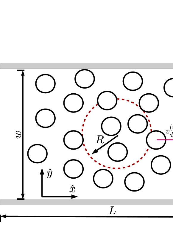
Figure 1: Schematic diagram for individuals in the corridor. The circles represent pedestrians moving from left to right. $w$ represents the corridor width, $L$ represents the length. The rectangular boxes are upper and lower blocks that represent the walls of the corridor. The dashed circle in the middle corresponds to the fundamental diagram measurement region.

2.3 Clustering structures

A characteristic feature of pedestrian dynamics is the formation of clusters. Clusters of pedestrians can be defined as the set of individuals that for any member of the group (say, $i$) there exists at least another member belonging to the same group ($j$) in contact with the former. Thus, we define a “granular cluster” ($C_{g}$) following the mathematical formula given in Ref. [7]

$$C_{g}:P_{i}~{}\epsilon~{}C_{g}\Leftrightarrow\exists~{}j~{}\epsilon~{}C_{g}/r_{ij}<R_{i}+R_{j},$$ (9)

where ($P_{i}$) indicates the ith pedestrian and $R_{i}$ is his (her) radius (shoulder width). That means, $C_{g}$ is a set of pedestrians that interact not only with the social and the desired forces, but also with granular forces (i.e. friction forces). The size of the cluster is defined as the number of pedestrians belonging to it. The fraction of clustered individuals is defined as the ratio between clustered individuals with respect to the total number of individuals in the crowd. In Section 5.7 we analyze the clustering structures in terms of these two observables.

3 Setting and parameters

We explored the flow of pedestrians along a straight corridor of length $L=$ 28 m (with periodic boundary conditions) and different values of the width $w$. We explored widths ranging from $w=2$ m to $w=40$ m. The corridor had two side walls, placed at $y=0$ and $y=w$, respectively. The length of each wall was $L$. The pedestrians were modeled as soft spheres of radius $R_{i}=0.23$ m. This size was fixed according to Ref. [36]. Initially, the individuals were randomly distributed along the corridor with a fixed global density (number of pedestrians over area) and with random initial velocities, resembling a Gaussian distribution with null mean value. We explored global density values in the range 1 p m^-2 $<\rho<$ 9 p m^-2. We did not explore extreme densities (say $\rho>$9 p m^-2) because we excluded injuring situations. The number of pedestrians in the simulation was given by the global density and the corridor dimensions chosen in each case.

In this work we use the common value $\kappa=2.4\times 10^{5}$ Kg m^-1 s^-1, but we eventually set the newly defined parameters $\kappa_{i}=2.4\times 10^{6}$ Kg m^-1 s^-1 and $\kappa_{w}=2.4\times 10^{6}$ Kg m^-1 s^-1, being $\kappa_{i}$ and $\kappa_{w}$ the pedestrian-pedestrian friction coefficient and the pedestrian-wall friction coefficient, respectively.

The desired velocity for each pedestrian $i$ was $\vec{v}_{d}^{~{}(i)}=1$ m s^-1 $\hat{e}_{d}^{~{}(i)}$, where the target $\hat{e}_{d}^{~{}(i)}$ was set as $\hat{e}_{d}^{~{}(i)}=(L,y_{i})\left\|(L,y_{i})\right\|^{-1}$, being $L$ the x-location of the end of the corridor and $y_{i}$ the y-location corresponding to the ith pedestrian (see Fig. 1). This allowed the pedestrians to move from left to right in a unidirectional flow. Pedestrians that surpassed $x=L$ were re-injected at $x=0$, preserving their current velocity and y-location (i.e. periodic boundary conditions). This mechanism was carried out in order to keep the crowd size unchanged.

We warn the reader that, for simplicity, we will not include the units corresponding to the numerical results. Remember that the friction coefficient has units $\left[\kappa\right]=$Kg m^-1 s^-1, the density $\left[\rho\right]=$p m^-2 and the flow $\left[J\right]=$p m^-1 s^-1.

3.1 Simulation software

The simulations were implemented on LAMMPS molecular dynamics simulator with parallel computing capabilities [37]. The time integration algorithm followed the velocity Verlet scheme with a time step of $10^{-4}$ s. All the necessary parameters were set to the same values as in previous works (see Refs. [9, 38]), except for the friction coefficient $\kappa$ and the radius $R_{i}$.

We implemented special modules in C++ for upgrading the LAMMPS capabilities to perform the SFM simulations. We also checked over the LAMMPS output with previous computations (see Refs. [6, 7, 8, 11, 12]).

The measurements were taken once the system reached the stationary state ($t=30$ s), while the configurations of the systems were recorded every 0.05 s, that is, at intervals as short as 10% of the pedestrian’s relaxation time (see Section. 2.1). The recorded magnitudes were the pedestrian’s positions and velocities for each process. We also computed the clustered structures using a LAMMPS built-in function named “compute cluster-atom”. This function assigns each pedestrian a cluster ID. A cluster is defined as a set of pedestrians, each of which is within the cutoff distance from one or more other pedestrians in the cluster. The cutoff was set as $R_{i}+R_{j}$ to assimilate the LAMMPS built-in function with the cluster definition given in Eq. (9). If a pedestrian has no neighbors within the cutoff distance, then it is a 1-pedestrian cluster.

4 Hypotheses

We stress the fact that our investigation focuses on moving pedestrians in a high density situation (say, the one experienced at the Jamaraat bridge). As mentioned in Section 1, a deep examination of the (basic) SFM parameters is required before proceeding to any extension of the model.

Recall from the video analysis of the Muslim pilgrimage in Mina/Makkah (see Section 1) that high-density flows can attain zero velocity, as people start pushing to gain space [1]. This unexpected behavior can not be reproduced by the (basic) SFM, it might happen because of “an underestimation of the local interactions triggered by high densities” [39], or, the absence of a “delayed reaction in cases of unexpected behaviors” [30]. Both statements are currently working hypotheses since experimental data (specifically, measurements of pedestrian flux and densities) do not “provide any insight into the mechanisms and dynamics behind the pedestrians interactions and behaviors” [30].

Researchers propose a “re-calibration” of the (basic) SFM, in order to attain “stop-and-go” flows for highly dense crowds [30, 39]. Presumably, this kind of instabilities within the crowd prevent people from stopping at extremely high densities. The intended “re-calibration” consists of either enhancing the (local) social interactions or increasing the net-time headway (roughly, the relaxation time) for the high density regime. Both extensions, however, may not exclude other possibilities involving not only individual motion but collective (mass) motion [1]. Researchers further point out that the relevance of physical contact in extremely dense crowds may suppose a somewhat commonality with granular media exists [1].

We show that the experimental data (say, the flux-density diagram) can be modeled under quasi-stationary conditions in the high density regime.

Our starting point will be the re-examination of the (basic) SFM. We propose a reduce-in-units equation of motion of the SFM (see Section 5.4 for details). From this point of view, the parameter $A$ standing for the intensity of the social force $\mathbf{f}_{s}$ is replaced by the reduced-in-units parameter $\mathcal{A}$. The friction intensity $\kappa$ of the granular force $\mathbf{f}_{g}$ is replaced by the reduced-in-units parameter $\mathcal{K}$. No other parameters are required in the reduced-in-units model since $m$, $v_{d}$, $\tau$ and $B$ are all included in $\mathcal{A}$ and $\mathcal{K}$. The desired force $\mathbf{f}_{d}$, indeed, will only depend on the target direction. In Section 5.4 we derivate the reduce-in-units equation of motion and the meaning of the control parameters ($\mathcal{A}$ and $\mathcal{K}$).

We presume that physical contact is a key feature in dense crowds, despite the fact that other issues may also contribute to the flow reduction [27]. However, the latter could be satisfactorily omitted in past research [30], and thus, we will not attempt to introduce further extensions to the (basic) SFM for the sake of simplicity.

The former “re-calibrations” accomplish the socio-psychological response of the crowd to “gain more space” (by either enhancing local interactions or performing a delayed reaction). We are aware that crowds may respond differently in many situations (see Ref. [40]). Our working hypothesis, however, does not focus on the crowd socio-psychological response, but on the physical contact among pedestrians (and the walls). The socio-psychological attitude of the pedestrians will be assumed to remain fixed along the simulations (with the desired speed limited to $v_{d}=1\,$ m s^-1).

Our investigation appears somewhat restricted to the (almost) unidirectional flow inspired from the Muslim pilgrimage in Mina/Makkah. This means that the following “re-calibration” results hold for corridor-like situations, and are not intended to be (automatically) translated to bottleneck situations. Neither can be extended to other boundary conditions (say, no limiting walls) since the boundary is a key feature of collective motion. Nevertheless, our results accomplish the available data on the Hajj pilgrimages [1, 20].

5 Results

5.1 Fundamental diagram in the original model

In this Section we present the results relating the local flow, velocity and density (i.e. the fundamental diagram). The measurements were taken in the middle of the corridor using the definitions given in Eq. (7), Eq. (8), and as shown in Fig. 1. All the results shown here correspond to $R=1$ m (see Eq. (8) and Fig. 1). We further varied $R$ until $R=3$, but no significant changes were observed.

Fig 2, shows the fundamental diagram (flow vs. density) for different corridor widths. We can distinguish the two typical regimes of the fundamental diagram. In the free flow regime ($\rho<5$), the flow increases linearly with the density since collisions between pedestrians (and with the walls) are scarce. Pedestrians are able to achieve their desired velocity, leading to a flow that grows linearly with the density ($J\propto\rho$) until $\rho=5$. This behavior applies to all the analyzed corridor widths.

On the other hand, we have the congested branch for $\rho>5$. Here we face two different scenarios:

• For narrow corridors (say $w<10$) we can see that the flow reduces as the density increases. This resembles the traditional behavior of the fundamental diagram reported in the literature.

• For wide corridors (say $w>15$) we see that the flow increases with density. This contradicts the typical behavior of the fundamental diagram.

In the case of narrow corridors, both the simulated case and the empirical results converge to a constant flow value. It is remarkable that the system does not reach a freezing state such as the one reported in Refs. [26, 41]. Recall that our simulations do not include any respect factor (see Ref. [28]), or changes in the net-time headway (Ref. [1]), or the urge to see an attraction (Ref. [26]). We assume a well-defined target and the same $v_{d}$ for all the pedestrians.

The inset in Fig. 2 corresponds to the empirical data from Helbing (see Ref. [1]) at the entrance of the Jamaraat bridge (the corridor width was $w=22$ m). Notice that our results from simulations corresponding to a $w=22$ m corridor, exhibit a different behavior along the congested regime. In the results from simulations, the flow increases even for the highest explored density. On the contrary, the empirical data exhibit a flow reduction for $\rho>5$ until reaching a plateau for the highest explored density values.

In order to fulfill the experimental fundamental diagram, it becomes necessary that the flow at the maximum explored density ($\rho_{max}=9$) does not exceed the flow at $\rho=5$ (upper bound). That is: $J(\rho=9)<J(\rho=5)$. From the flow definition in Eq. (8) we can derive the bounding values

$$v(\rho_{max})<\frac{5v_{d}}{\rho_{max}}\leq\frac{5}{9}v_{d},\\$$ (10)

As our desired velocity is fixed at $v_{d}=1$ m s^-1, we conclude that the speed at the maximum density has to be bounded by $v(\rho_{max})\lesssim 0.5$ m s^-1 in order to satisfy the qualitative behavior of the (experimental) fundamental diagram reported in the literature.

The above reasoning is consistent with the speed-density results shown in Fig. 3. As a visual guide, we plotted $v=0.5$ m s^-1 with a horizontal dashed line. The close examination of $\rho_{max}=9$ shows that values corresponding to the wide corridors ($w=15$ m and $w=22$ m) exceed $v=0.5$ m s^-1. But, those values corresponding to narrow corridors fall below $v=0.5$ m s^-1.

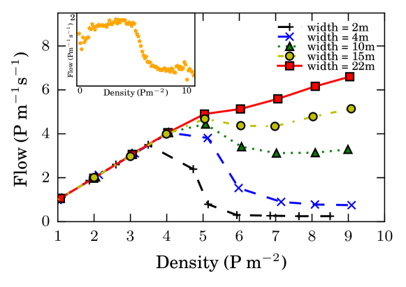
Figure 2: Mean flow ($J$) as a function of the density ($\rho$) for different widths. Initially, pedestrians were randomly distributed along the corridor. The measurements were taken in the middle of the corridor once the system reached the stationary state (see Fig. 1). The length of the corridor was $L=$28 m for all cases (with periodic boundary conditions in the x direction). The inset corresponds to Ref. [1]

The results shown in Fig. 3 confirm the fact that when the density is low enough, pedestrians manage to walk at the desired velocity ($v=v_{d}=1$ m s^-1). Above $\rho>5$, however, the velocity begins to slow down. The inset shows the experimental data at the entrance of the Jamaraat bridge. We may conclude that our simulations agree with the experimental data for narrow corridors, but disagree as these become wider. The wider the corridor, the greater the velocity for all the density values explored. In Section 5.2 we will further discuss this topic.

It should be pointed out that the Jamaraat data do not exhibit a “really” constant velocity for low densities. But this seems reasonable since our simulations do not include the complexities of the real situation when the density is low. We will not analyze this phenomenon in this investigation.

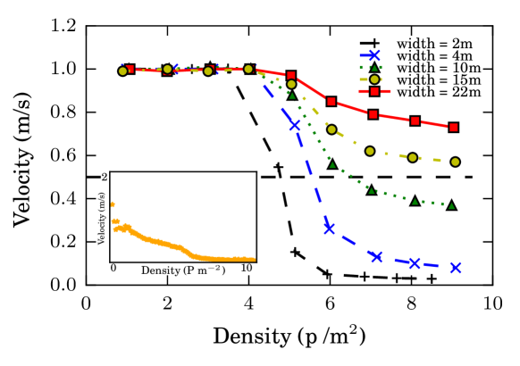
Figure 3: Mean speed ($V$) as a function of the density ($\rho$) for different widths. Initially, pedestrians were randomly distributed along the corridor. The measurements were taken in the middle of the corridor once the system reached the stationary state (see Fig. 1). The length of the corridor was 28 m in all cases (with periodic boundary conditions in the x-direction). The inset corresponds to Ref. [1].

We may summarize our first results as follows. We were able to validate the original SFM for narrow corridors through the fundamental diagram. However, the SFM (in its current version) disagrees with experimental data as the corridors widen. We will focus in the next Section on the velocity profile in order to investigate this discrepancy.

5.2 Velocity profile

As we mentioned in Section 5.1, when the density is low, pedestrians achieve the desired velocity ($v=v_{d}=1$ m s^-1). Since the results of the previous Section only hold for the area located in the middle of the corridor (see the dashed circle in Fig. 1), we want to shed some light and understand what is happening across the entire corridor.

We first noticed that low-density situations ($\rho<5$) lead to a cruising velocity profile $v=v_{d}$. This is valid for every location in the corridor (not only the center as was previously noticed in Section 5.1). For higher densities ($\rho>5$), the velocity profile turns into a parabola-like function. This shape resembles the usual velocity profile for laminar flow in a viscous fluid, where the velocity increases toward the center of a tube. In our case, pedestrians near the walls are the ones with the lower velocity. The velocity increases when departing from the wall until it reaches the maximum at the center of the corridor. This behavior suggests that the wall friction on the pedestrians, is playing a relevant role in the velocity distribution. The velocity profile is in agreement with the empirical data in Ref. [42].

Fig. 4 exhibits the scaled velocity profile. The horizontal axis is normalized by the corresponding corridor width. The vertical axis is normalized by the maximum velocity ($v_{max}$) corresponding to each data set. Filled markers correspond to density $\rho=9$, while empty markers correspond to $\rho=6$. Notice that all the data follow the same pattern, suggesting that the velocity profile exhibits a somewhat fundamental behavior, regardless of the scale of the corridor (and the density). Hence, the velocity growth rate from the wall towards the center of the corridor is the same in spite of the size of the corridor width and the density.

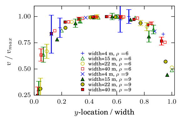
Figure 4: Scaled velocity profile (normalized velocity) vs. $y$-location for different corridors width (see legend for the corresponding widths) and two different densities. Empty markers correspond to $\rho=6$ while filled markers correspond to $\rho=9$. The simulated corridor was 28 m length. Pedestrians walk from left to right with periodic boundary condition in the $x$-direction. Initially, pedestrians were randomly distributed. The horizontal axis is normalized by the corridor width, the vertical axis is normalized by the maximum velocity reached in each case. The bin size was 1 m for all cases except for $w=4$ m since the bin was 0.5 m.

We remark that there is a clear relation between $v_{max}$ and the corridor width. That is, the wider the corridor, the higher the maximum attained velocity (Fig. 4 does not exhibit this behavior because the velocity is normalized by $v_{max}$).

In summary, the scaled velocity profile (see Fig. 4) does not report any relevant difference as the corridor widens (withing the high density regime). This suggests that the pedestrian dynamics remain essentially the same. The maximum attainable velocity ($v_{max}$), however, seems to be a sensible parameter with respect to the flux. The narrow corridors attain lower values of $v_{max}$ and thus lower flux. We may expect the flow not to increase if $v_{max}$ remains low enough along the explored density range.

5.3 Work done by friction force

In the previous Section we studied the velocity profiles for different corridors as a function of density. Here we present the spatial distribution of the work done by the friction force. The pedestrian-pedestrian friction and the pedestrian-wall friction were computed. The work on each pedestrian $i$ was numerically obtained through the integration Trapezoidal rule (according to Eq. 11). The integration time step was $\Delta t=0.05$ s.

$$W^{(i)}(t)\simeq\left[\vec{f}^{(i)}(t+\Delta t)+\vec{f}^{(i)}(t)\right]\cdot\frac{\Delta\vec{x}}{2}.$$ (11)

Once the work on every pedestrian is calculated, we proceeded to bin the corridor into a squared grid of 1 m$\times$1 m cells in order to associate the work values with the corresponding spatial location. Fig. 5 shows three color maps of the absolute value of the work done by the friction force. The horizontal and vertical axis represent the $x$-location and $y$-location of the corridor respectively. The color map associates higher work values with red colors and lower work for blue colors. The walls are located at $y=0$ and $y=w$ (bottom and top of each figure). Fig. 5a corresponds to a 10 m width corridor, Fig. 5b corresponds to a 15 m width corridor and Fig. 5c corresponds to a 22 m width corridor.

In the three figures, we observe a similar pattern: the regions near the walls (bottom and top) are the most dissipative ones. The center of the corridor is though not a very dissipative region. Furthermore, the work seems to increase with the corridor width. This occurs because the relative velocity between pedestrians is greater in the wide corridors than in the narrow ones. The wider the corridor, the greater the slope (corresponding to locations near the wall).

Recall from Eq. (3), that the friction force depends on the compression and the relative velocity among pedestrians. The compression levels remain the same in the three cases since the compression only depends on the density (which is fix at $\rho=6$ for the three color maps). Thus, the differences between Figs. 5a, 5b and 5c can only be explained by the increment of the relative velocity between individuals.

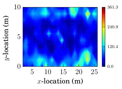
(a)

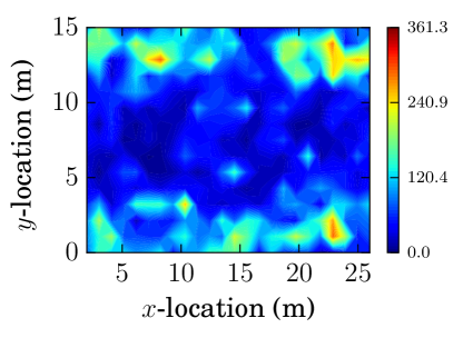
(b)

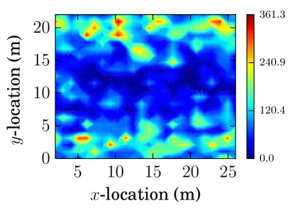
(c)

Figure 5: Color map for the absolute value of the work done by the friction. The density chose was $\rho=6$. (a) Corresponds to $w=$10 m (b) $w=$15 m and (c) $w=$22 m. The axis represent the location in the corridor ($x$ and $y$). The scale bar on the right is expressed in Joule units. The work was numerically integrated following the Trapezoidal rule with $\Delta t=0.05$ s. The pedestrians desired velocity was $v_{d}=1$ m s^-1. The contour lines were computed on a square grid of 1m$\times$ 1m and then splined to get smoother curves.

The above observations drive the following conclusion. The maximum attainable velocity $v_{max}$ accomplishes a maximum velocity slope (with its associated friction dissipation). Both the friction with the walls and the friction between the pedestrians appear as relevant magnitudes for properly slowing down the crowd velocity, in order to fit the experimental data. Section 5.5 supports this assertion with a simple example.

5.4 The reduced equation of motion

The equation of motion within the context of the SFM includes at least six parameters ($m$, $\tau$, $A$, $B$, $\kappa$ and $v_{d}$), but the equation itself barely depends on two. The process of parameter’s reduction is achieved by defining the (reduced) magnitudes

$$\left\{\begin{array}[]{lll}t^{\prime}&=&t/\tau\\ r^{\prime}&=&r/B\\ v^{\prime}&=&v/v_{d}\\ \end{array}\right.$$ (12)

The (reduced) equation of motion reads

$$\frac{d\mathbf{v}^{\prime}}{dt^{\prime}}=\displaystyle\frac{\tau}{m\,v_{d}}\bigg{(}\mathbf{f}_{d}+\mathbf{f}_{s}+\mathbf{f}_{g}\bigg{)}.$$ (13)

It is straight forward from Eq. (13) that the corresponding reduced forces can be defined as follows

$$\left\{\begin{array}[]{lll}\mathbf{f}_{d}^{\prime}&=&\hat{\mathbf{e}}_{d}-\mathbf{v}^{\prime}\\ &&\\ \mathbf{f}_{s}^{\prime}&=&\mathcal{A}\,\exp(r^{\prime}-d^{\prime})\,\hat{\mathbf{n}}\\ &&\\ \mathbf{f}_{g}^{\prime}&=&\mathcal{K}\,(2r^{\prime}-d^{\prime})\,\Theta(2r^{\prime}-d^{\prime})\,(\Delta\mathbf{v}^{\prime}\cdot\hat{\mathbf{t}})\ \par\hat{\mathbf{t}}\\ \end{array}\right.$$ (14)

where $\mathcal{A}=A\tau/(m\,v_{d})$ and $\mathcal{K}=\kappa B\tau/m$.

Notice that $\mathcal{A}$ and $\mathcal{K}$ are actually the only two control parameters in Eq. (13) for identical pedestrians. The ratio $\tau/m$ is common to both, but the magnitudes $Av_{d}^{-1}$ and $\kappa B$ handle each parameter separately.

We envisage $\mathcal{A}$ as a parameter related exclusively to the repulsion between pedestrians and $\mathcal{K}$ as a parameter related to the friction-repulsion. While the former is valid in every situation, the latter only takes part when the pedestrians are in contact.

The fact that $\mathcal{A}$ and $\mathcal{K}$ share the parameter $\tau$ is in agreement with the conclusions outlined in Ref. [30]. The relaxation time (or “net-time headway”) $\tau$ actually “weights” the effects of the environment on the individual (that is, the social repulsion and the friction), and thus, appears as a “key control parameter” for the fundamental diagram as claimed in Ref. [30].

The role of $\tau$ may be somewhat ambiguous whenever the social repulsion becomes negligible with respect to the friction. This may occur if some kind of balance exists between neighboring pedestrians in symmetrical configurations (i.e. in crowded corridors). We may hypothesize that the “key control parameter” may correspond to either $\tau$, or, the friction itself $\kappa$. This is an open question, and a first order approach to this matter is outlined in Section 5.5.

5.5 A simple model for the corridor

A toy model for a moving crowd along a corridor is the one represented schematically in Fig. 6. Pedestrians (circles in Fig. 6) are assumed to be lined up from side to side across the corridor, at any given position. Social forces in the $x$-direction are further considered to vanish because of the translational symmetry. Thus, only the sliding friction is allowed to balance the pedestrians own desire. The (reduced) movement equation for the $x$-direction according to Section 5.4 and Fig. 6 is

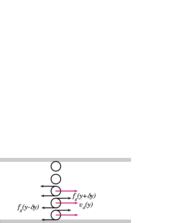
Figure 6: Schematic diagram for individuals in a corridor. The circles represent pedestrians moving from left to right. The desired force (red arrows) and sliding friction (black arrows) are assumed to be the only relevant forces.

$$\frac{dv^{\prime}}{dt^{\prime}}(y^{\prime})=1-v^{\prime}(y^{\prime})+f_{g}^{\prime}(y^{\prime}+\delta y^{\prime})-f_{g}^{\prime}(y^{\prime}-\delta y^{\prime}),$$ (15)

where $v^{\prime}(y^{\prime})$ corresponds to the (reduced) velocity (for the $x$-direction) of the individual located at the $y^{\prime}$ position. Notice that the individuals remain at the same $y^{\prime}$ position while traveling through the corridor since balance is expected to take place across the corridor. These positions are roughly $\delta y^{\prime}$, $3.\delta y^{\prime}$, $5.\delta y^{\prime}$,…. Actually, it is not relevant (for now) the value of $y^{\prime}$, and a further simplification can be done by labeling $v^{\prime}(y^{\prime})=v_{i}$ and $v^{\prime}(y^{\prime}\pm 2.\delta y^{\prime})=v_{i\pm 1}$. The velocity of the individual in contact with the bottom wall in Fig. 6 will be labeled as $v_{1}$.

The last two terms in Eq. (15) correspond to the net drag applied on the pedestrian with velocity $v_{i}$. According to Eq. (14) this drag may be expressed as

$$f_{g,i+\frac{1}{2}}^{\prime}-f_{g,i-\frac{1}{2}}^{\prime}=\left\{\begin{array}[]{lcl}2\alpha\,v_{2}-3\alpha\,v_{1}&&i=1\\ &&\\ 2\alpha\,(v_{i+1}-2v_{i}+v_{i-1})&&i>1\\ \end{array}\right.$$ (16)

for $\alpha=\mathcal{K}(r^{\prime}-\delta y^{\prime})$. Recall that our first order approach considers $\delta y^{\prime}$ as roughly uniform across the corridor.

The stationary situation can be computed straight forward from Eq. (15). Thus, for $\dot{v}_{i}=0$ the following set of equations determine the velocity profile in the corridor (within this toy model)

$$\left\{\begin{array}[]{lcl}(3\alpha+1)\,v_{1}-2\alpha\,v_{2}&=&1\\ &&\\ -2\alpha\,v_{i-1}+(4\alpha+1)\,v_{i}-2\alpha\,v_{i+1}&=&1\\ \end{array}\right.$$ (17)

Notice from Eq. (16) that $\alpha=0$ means no friction at all, and thus, the individuals are allowed to move free from drag. It can be verified that $v_{i}=1$ solves the set (17) for this scenario. The $\alpha=0$ scenario is expected to occur, however, for densities below a contacting threshold.

A boundary condition needs to be imposed in order to solve Eq. (17) for $\alpha\neq 0$. We fix $v_{i}=v_{i+1}$ in the middle of the corridor since the velocity profile should be symmetrically distributed with respect to the mid-axis of the corridor. Fig. 7 shows the computed mean velocity for the bottom side profile as a function of $\alpha$.

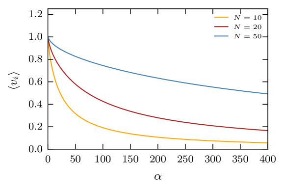
Figure 7: Mean velocity of the bottom half of the individuals vs. the parameter $\alpha$. Both axis are dimensionless. $N$ corresponds to the number of individuals.

Fig. 7 exhibits a decreasing behavior for increasing values of $\alpha$. As explained above, the maximum value occurs at $\alpha=0$ (i.e. $\langle v_{i}\rangle=1$). However, the decreasing slope slows down for an increasing number of individuals. This corresponds to a flattening in the velocity profile (see Section 5 for details).

The mean flux of individuals can be built from the mean velocity and the corresponding pedestrian density as follows

$$J=\left\{\begin{array}[]{lcl}\rho&\mathrm{for}&\alpha=0\\ &&\\ (\rho_{0}+c\,\alpha)\,\langle v_{i}\rangle&\mathrm{for}&\alpha>0\\ \end{array}\right.$$ (18)

where $\langle v_{i}\rangle$ equals unity for the case $\alpha=0$, and thus, it was omitted in (18). The density $\rho=\rho_{0}+c\,\alpha$ corresponds to the packing density (that is, the density above the contacting threshold) and $c$ corresponds to a somewhat “packing coefficient”. Fig. 8 shows the flow as a function of the density, assuming $\rho_{0}=1$ for simplicity.

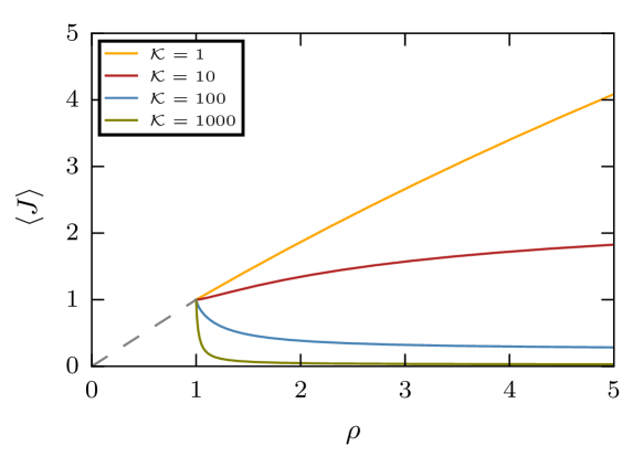
Figure 8: Mean flux of the bottom half of the individuals vs. the pedestrian (global) density $\rho$ (see text for details). Both axis are dimensionless. The number of individuals across the corridor was set to $N=10$ and the contacting threshold was set to $\rho_{0}=1$. The “packing coefficient” was set to $c=1/\mathcal{K}$ (and thus, making the term $c\alpha$ independent of friction). The dashed line corresponds to the flux at the low density regime (say, $\langle v_{i}\rangle=1$).

The pedestrian flux $J$ attains two possible behaviors, according to Fig. 8. For packing coefficients $c<0.05$, the flux diminishes as the corridor becomes more crowded. But, if $c$ surpasses this threshold, the flux slope becomes positive, although the mean velocity diminishes. We conclude that the role of the pedestrians’ friction coefficient is crucial for building the fundamental diagram.

5.6 Friction modification

As already mentioned, the results shown so far indicate that friction may be the key magnitude for fitting the fundamental diagram into the experimental data. We want to make clear that fitting the experimental data means mimicking (qualitatively) the congested regime reported by different authors (including the Jamaraat study in Ref. [1]) for corridors as width as 22 m. The original version of the SFM proposes the same friction coefficient for the pedestrian-pedestrian interaction and the pedestrian-wall interaction. The proposed value was $\kappa=2.4\times 10^{5}$. This value is widely used in many studies.

We tested the friction coefficient modification in Section 5.5 and we found that the fundamental diagram experiences a qualitatively change when the friction coefficient $\kappa$ is varied. We further performed numerical simulations in the context of the SFM. We call $\kappa_{i}$ as the friction coefficient of the pedestrian-pedestrian interaction and $\kappa_{w}$ as the friction coefficient of the pedestrian-wall interaction. Fig. 9 shows the flow vs. density for different values of $\kappa_{i}$ and $\kappa_{w}$.

The triangular symbols in Fig. 9 correspond to the increase in one order of magnitude of the wall friction (now $\kappa_{w}=2.4\times 10^{6}$), leaving the pedestrian-pedestrian friction unchanged (i.e., $\kappa_{i}=2.4\times 10^{5}$). We can see that the flow reduces a little bit, but this is not enough to change significantly the congested regime.

The circles in Fig. 9 correspond to a modification of the friction between pedestrians without changing the value of the wall friction. We increased the pedestrian-pedestrian friction by a factor of ten ($\kappa_{i}=2.4\times 10^{6}$). Here we see a significant reduction of the flow. The qualitative behavior resembles the fundamental diagram reported by Helbing et al [1]. with a well defined congested regime for the greatest densities.

We also tested the case were both friction coefficients surpass ten times the value of the original model (now $\kappa_{w}=\kappa_{i}=2.4\times 10^{6}$). The squared symbols represent this scenario. As expected, the flow reduces significantly with respect to the original case (cross symbol). Interestingly, the reduction of the flow is more than the reduction due to the increment of $\kappa_{i}$ plus the reduction of the flow due to $\kappa_{w}$. This behavior indicates that the superposition principle does not hold in this system because of the non-linearity of the equation of motion.

This finding allows us to affirm that the friction plays a crucial role in the functional behavior of the fundamental diagram. The increment of both individual-individual friction and wall friction are determinant in order to achieve a congested regime. More specifically, the empirical behavior for the fundamental diagram can be achieved by properly increasing the friction coefficients. In A we show that the friction modification does not alter already studied behaviors of pedestrian dynamics.

Recall that other authors address the “congested regime problem” by modifying different aspects of the model. Ref. [28] imposes zero desired velocity once pedestrians are close enough, Ref. [30] increases the relaxation time in order to slow down the net-time headway, and more recently, Ref. [26] induce the jamming transition by an attraction. Many of these approaches seem to be equivalent. In Section 5.4 we discuss how the modification of the relaxation time and the increment of the friction coefficient yield a similar effect since both affect the same term in the reduced-in-units equation of motion. The relaxation time, however, also affects the social interactions (see Sections 4 and 5.4).

We claim that in real scenarios, a combination of all these factors may be the cause of the marked flow reduction that portrays the fundamental diagram. The pedestrians path can be very complex even if it is a simple enclosure (straight corridor) and the target is well defined (unidirectional flow). Beyond the complexities given by the internal motivations of pedestrians, we strongly suggest studying and modeling coefficients of friction between individuals and the friction with the walls. These two parameters have shown to be very important in the pedestrian dynamics and deserve a closer inspection in future research.

We want to emphasize that the proposals stated in Refs. [26, 28, 30] only apply under normal conditions. If a crowd is under high levels of anxiety, pedestrians will neither keep distance between each other nor will feel the urge to see an “attraction”. Thus, studying the friction coefficients may be a critical factor to properly reproduce the dynamics of a massive evacuation under stress.

With all these insights, we can say that the narrow corridors have no drawbacks in the fitting of the flow vs. density because very high velocities are not attainable. This happens because, in narrow corridors, the friction of the walls has a lot of “relative weight” in the overall friction of the system. The friction exerted by the walls is fundamental in order to produce the parabolic shape of the velocity profile. The walls provide friction force in the opposite direction to the speed of the individual (drag backwards), since they act like a fixed pedestrian. In other words, friction between pedestrians can produce either drag forward or drag backwards depending on the contacting pedestrians velocities (see Eq. 3).

Figure 9: Fundamental diagram (flow vs. density) for different friction coefficient (see legend for the corresponding values). The simulated corridor was 28 m length. Pedestrians walk from left to right with periodic boundary condition in the $x$-direction. Initially, pedestrians were randomly distributed. For each density, we measure the flow once the system reaches the stationary state.

In this subsection, we have shown that an adequate modification of the friction coefficients yields a fundamental diagram that follows qualitatively the behavior reported through empirical data (say flow reduction for the highest densities). We have also discussed different approaches proposed by other authors in order to overcome this problem. See Section 5.4 for a more detailed discussion.

5.7 Clusters

Cluster formation is a very important process in pedestrian dynamics. Moreover, it is the key process that explains the clogging phenomena in bottleneck evacuations. We analyzed the clustering formation according to the granular cluster definition given in Section 2.3. Fig. 10 shows the histograms of the cluster size distribution for three different densities, from top to bottom: $\rho=4.5$, $\rho=5$ and $\rho=5.5$. These three densities are representative of the crossover between a non-clusterized regime and a unique giant cluster regime. We studied two situations for each density: the original SFM on the left hand side plots, and the enhanced friction situation on the right hand side plots (see the caption for details).

We found two unexpected results. Increasing the density produces bigger size clusters until the size distribution suddenly switches to a bimodal distribution (compare Fig. 10c with Fig. 10e and Fig. 10b with Fig. 10d). Once this phenomenon occurs, any of two possibilities may appear: the pedestrian belongs to a small cluster (out of many “caged” in the crowd) or he (she) belongs to the giant cluster (with a size comparable to the entire crowd). In other words, the bimodal distribution occurs because, after the giant component is formed, many small clusters remain “caged” inside the giant component. These small clusters (or single individuals) do not touch permanently any pedestrian belonging to the giant component.

We also observed that this phenomenon is controlled by the friction. For higher frictions, the crossover to the bimodal distribution occurs at lower densities (see Fig. 10c and Fig. 10d). Despite the fact that both correspond to the same density, Fig. 10d already attains the bimodal distribution since the friction force is ten times greater than in Fig. 10c. This peculiar phenomenon occurs because in an enhanced friction scenario the individuals find it harder to detach from each other. On the opposite, when the friction is weak, the individuals detach themselves more easily, leading to a situation where large clusters are less probable.

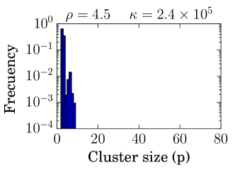
(a)

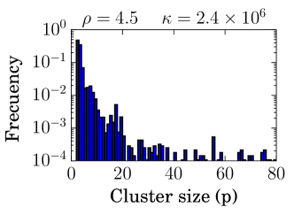
(b)

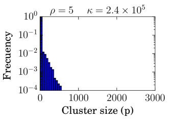
(c)

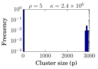
(d)

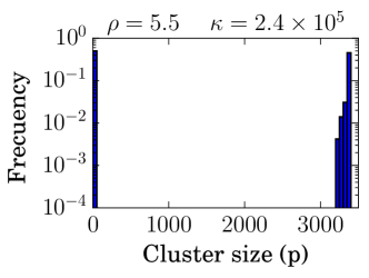
(e)

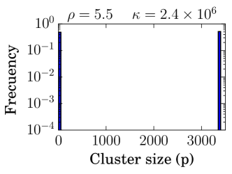
(f)

Figure 10: Cluster size distribution for six different scenarios. (a) SFM friction parameters and $\rho=4.5$, the bin size is 1 p (b) friction parameters increased by a factor of ten and $\rho=4.5$, the bin size is 1 p (c) SFM friction parameters and $\rho=5$, the bin size is 50 p (d) friction parameters increased by a factor of ten and $\rho=5$, the bin size is 50 p (e) SFM friction parameters and $\rho=5.5$, the bin size is 50 p (f) friction parameters increased by a factor of ten and $\rho=5.5$, the bin size is 50 p.

To get a better view of this phenomenon, we represent in Fig. 11 the fraction of clustered individual as a function of the density for four different situations in which we only changed the friction coefficients. The fraction of clustered individuals is defined as the amount of pedestrians that belong to a cluster (of two or more individuals) over the total number pedestrians in the corridor. We can see that there is a transition from a non-clustered crowd to a full-clustered crowd. This transition occurs in a very narrow range of densities, causing the cluster formation process to occur between $4.4<\rho<5.3$. When the friction coefficient is enhanced, the transition takes place at a lower density threshold. This result is in complete agreement with the histograms shown in Fig. 10, confirming the fact that friction promotes the formation of clusters.

As expected, the transition sharpens when both $\kappa_{i}$ and $\kappa_{w}$ are increased (squared symbol in Fig. 11). However, the fraction of clustered individuals is always greater than in the original SFM when just one of the two coefficients is increased. Notice that there is not a big difference between the modification of $\kappa_{i}$ and the modification of $\kappa_{w}$. This suggests that it does not matter if the clusterization starts at the areas close to the walls or in the middle of the crowd.

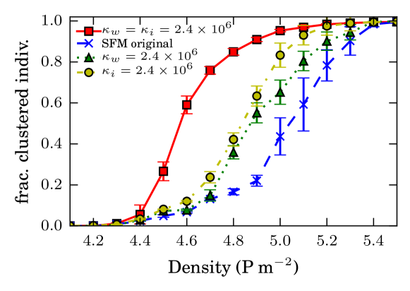
Figure 11: Fraction of clustered individuals as a function of the density. Squared symbols correspond to $\kappa_{w}=\kappa_{i}=2.4\times 10^{6}$, circles to $\kappa_{i}=2.4\times 10^{6}$ and $\kappa_{w}=2.4\times 10^{5}$, triangles to $\kappa_{i}=2.4\times 10^{5}$ and $\kappa_{w}=2.4\times 10^{6}$ and crosses to the coefficients of the original SFM ($\kappa_{i}=2.4\times 10^{5}$ and $\kappa_{w}=2.4\times 10^{5}$). The pedestrians walk across a corridor with $v_{d}=1$m s^-1. The measurements were recorded every 0.5 s once the system reached the stationary state. The values corresponding to the fraction of clustered individuals were averaged over 170 s. The cluster cutoff distance was 0.46 m (equivalent to the shoulder width of the pedestrians).

Two main conclusions can be outlined from the above results. The friction coefficients between the pedestrians (and with the walls) appear as decisive parameters with respect to the crossover between the freely moving regime and the slow down regime. The precise (density) threshold between both regimes will actually depend on the friction coefficients since these control the efforts required by the pedestrians to detach from each other. Above this threshold (say, at high densities) the whole crowd slows down since the pedestrians appear mostly clustered or “caged” in a clustered environment.

6 Conclusions

Our investigation focused on the fundamental diagram in the context of the SFM. We compared empirical data recorded at the entrance of the Jamaraat bridge (see Ref. [1]) with our own SFM simulations. We observed that the SFM, in its original version, does not properly reproduce the empirical fundamental diagram since the pedestrian flow increases even for highly dense crowds. The reasons for this mismatching were studied through numerical computations and by a simple theoretical example. We arrived at the conclusion that either increasing the friction coefficient or increasing the relaxation time it is possible to achieve a non-increasing flow in the congested regime of the fundamental diagram. The latter has already been explored in Ref. [30] and a similar idea was introduced in Ref. [28]. We noticed, though, that both approaches are equivalent since both affect the reduced-in-units equation of motion in a similar fashion.

In order to further explore the effect of the friction term on the dynamics of the crowd, we performed numerical simulations increasing the value of $\kappa$. We were able to reproduce the empirical fundamental diagram for sufficiently high values of $\kappa$, while keeping the original SFM unchanged (without incorporating neither additional forces nor extra parameters). This is actually the main achievement of our investigation.

We further explored the velocity profile across a corridor. It appears to follow a parabolic-like function. The pedestrians at the middle of the corridor attain the maximum velocity, while those close to the walls attain the minimum. We noticed that the velocity profiles, after been scaled by the maximum velocity $v_{max}$ and the corridor width $w$, yield a somewhat universal behavior, regardless of the corridor width. Thus, we worked on the hypothesis that the dynamics should be essentially the same for narrow or wide passageways.

The presence of clustering structures was found to be controlled by the friction coefficient. Interestingly, increasing the pedestrian-pedestrian friction ($\kappa_{i}$) or the pedestrian-wall friction coefficient ($\kappa_{w}$) yields a similar clusterization dependence with density.

All these phenomena suggest that further research needs to be done regarding the friction coefficient. The explored values introduced through the investigation, however, should not be considered as “empirical” ones. Its true meaning (within the context of the SFM) is related to the other parameters in the model (see Section 5.4). A real consensus on empirical values of $\kappa$ is still missing, to our knowledge. Further analyses are needed to fully explore this issue and are currently under development.

We further proposed modeling the pedestrian-wall friction interaction with a different coefficient than the pedestrian-pedestrian friction interaction. This does neither mean a “re-calibration” (for highly dense crowds) nor a departure from the original SFM model. We actually find no reason for changing other parameters, regardless of any specific situation. We also stress the fact that studying the friction coefficients may be a critical factor to properly reproduce the dynamics of a massive evacuation under high levels of anxiety.

Appendix A Testing out previous results

In this Appendix, we show that the friction modification does not alter already studied behaviors of pedestrian dynamics (see Refs. [6, 7, 8]). In order to check this out, we performed numerical simulations of a room of 225 pedestrians escaping through a narrow door (bottleneck enclosure). The evacuation time (clearance time) $t_{e}$ is a function of the desired velocity $v_{d}$. This function has a minimum such that below it, $t_{e}$ is a decreasing function of $v_{d}$ while above, the tendency is reversed. It means that the evacuation process is optimum at moderated $v_{d}$. This is a well known phenomenon called the Faster-is-Slower effect. This effect was reported in numerical simulations [7, 9] and it has also experimental support [43].

In Fig. 12 we show the evacuation time as a function of the desired velocity corresponding to a friction coefficient ten times greater than the friction coefficient of the original SFM (i.e. now $\kappa=2.4\times 10^{6}$). We can see that this modification preserves the Faster-is-Slower effect (and the Faster-is-Faster effect). The inset exhibits the evacuation time as a function of the desired velocity with the friction coefficient of the original model ($\kappa=2.4\times 10^{5}$).

Another pedestrian dynamics phenomenon is the lane formation reported in bidirectional flows [44, 45, 46, 47]. This means, individuals spontaneously organize in lanes of uniform walking direction if the pedestrian density is high enough. One of the major achievements of the SFM is its ability to reproduce this emergent phenomenon in which the microscopic interactions between pedestrians is enough to produce a global pattern. We run a bidirectional flow simulation (not shown) and verified that the friction increment still reproduces the lane formation process.

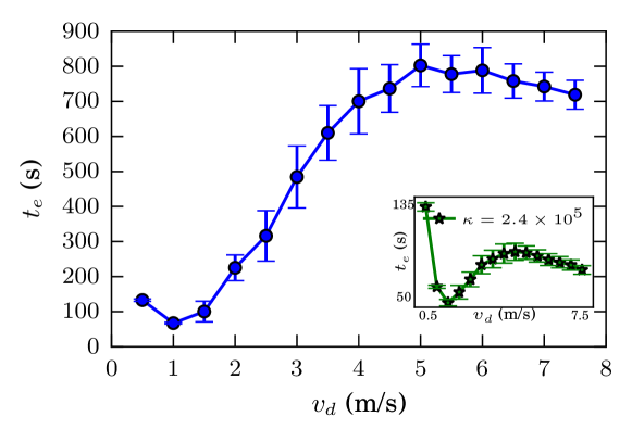
Figure 12: Mean evacuation time (seconds) vs. the pedestrian’s desired velocity (m s^-1). The room was 20 m $\times$ 20 m size. Mean values were computed from 30 evacuation processes. The pedestrians were initially placed in a regular square arrangement along the room with random velocities, resembling a Gaussian distribution with null mean value. The friction coefficient was $\kappa=2.4\times 10^{6}$. The inset shows the evacuation time vs. the desired velocity for the friction coefficient corresponding to the original model ($\kappa=2.4\times 10^{5}$).

Fig. 13 exhibits the ratio between the evacuation time for the friction modified model and the evacuation time for the original model. This ratio is shown as a function of the desired velocity. As the desired velocity increases, the rate of evacuation times approaches a constant value $\sim$ 9. This result is in agreement with the formula Eq. (9) in Ref. [38]. The friction force dominates in the range of high desired velocities since it promotes the collisions between pedestrians. Within this regime, the Eq. (9) of Ref. [38] becomes a good approximation of the evacuation time. Thus, it is reasonable that dividing $t_{e}(\kappa_{10})$ (for the enhanced friction) by $t_{e}$ (for the original model) yields a constant value for high $v_{d}$.

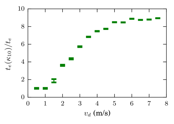
Figure 13: Rate of evacuation time ($t_{e}(\kappa_{10})/t_{e}$) vs. the desired velocity. The room was 20 m $\times$ 20 m size. Mean values were computed from 30 evacuation processes. The pedestrians were initially placed in a regular square arrangement along the room with random velocities, resembling a Gaussian distribution with null mean value. The friction coefficient were $\kappa=2.4\times 10^{6}$ and $\kappa=2.4\times 10^{5}$.

We also tested the situation in which $k_{i}=2.4\times 10^{6}$ and $k_{w}=0$. We obtained similar results to the ones obtained when $k_{i}=k_{w}=2.4\times 10^{6}$ because the friction of the walls in bottleneck evacuations do not play a fundamental role in the evacuation process.

References

- [1] Helbing, D., Johansson, A., and Al-Abideen, H. Z., 2007. “Dynamics of crowd disasters: An empirical study.” Physical review E 75 (4), 046109. https://doi.org/10.1103/PhysRevE.75.046109
- [2] Hirai, K., and Tarui, K., 1975. “A simulation of the behavior of a crowd in panic”, Proceedings of the 1975 International Conference on Cybernetics Society, pp. 409-411
- Okazaki [1979] Okazaki, S., 1979. “A study of pedestrian movement in architectural space, Part 1: pedestrian movement by the application of magnetic model”. Trans. A.I.J. 283, 111–119.
- [4] Helbing, D., Farkas, I., and Vicsek, T., 2000. “Simulating dynamical features of escape panic.” Nature 407.6803: 487-490. https://doi.org/10.1038/35035023
- [5] Helbing, D., and Molnár, P., 1995. “Social force model for pedestrian dynamics.” Physical review E 51 (5), 4282. https://doi.org/10.1103/PhysRevE.51.4282
- [6] Parisi, D. R., and Dorso, C. O., 2007. “Morphological and dynamical aspects of the room evacuation process.” Physica A: Statistical Mechanics and its Applications 385 (1), 343-355. https://doi.org/10.1016/j.physa.2007.06.033
- [7] Parisi, D. R., and Dorso, C. O., 2005. “Microscopic dynamics of pedestrian evacuation.” Physica A: Statistical Mechanics and its Applications 354, 606-618. https://doi.org/10.1016/j.physa.2005.02.040
- [8] Frank, G. A., and Dorso, C. O., 2011. “Room evacuation in the presence of an obstacle.” Physica A: Statistical Mechanics and its Applications 390 (11), 2135-2145. https://doi.org/10.1016/j.physa.2011.01.015
- [9] Sticco, I. M., Frank, G. A., and Dorso, C. O., 2017. “Room evacuation through two contiguous exits.” Physica A: Statistical Mechanics and its Applications 474, 172-185. https://doi.org/10.1016/j.physa.2017.01.079
- [10] Cornes, F. E., Frank, G. A., and Dorso, C. O., 2017. “High pressures in room evacuation processes and a first approach to the dynamics around unconscious pedestrians.” Physica A: Statistical Mechanics and its Applications 484, 282-298. https://doi.org/10.1016/j.physa.2017.05.013
- [11] Frank, G. A., and Dorso, C. O., 2015. “Evacuation under limited visibility.” International Journal of Modern Physics C 26.01, 1550005. https://doi.org/10.1142/S0129183115500059
- [12] Frank, G. A., and Dorso, C. O., 2016. “Panic evacuation of single pedestrians and couples.” International Journal of Modern Physics C 27.08, 1650091. https://doi.org/10.1142/S0129183116500911
- [13] Köster, G., Treml, F. and Gödel, M., 2013. “Avoiding numerical pitfalls in social force models.” Physical Review E 87 (6), 063305. https://doi.org/10.1103/PhysRevE.87.063305
- [14] Seyfried, A., Schadschneider, A., Wagoum, K., Ulrich, A. and Mohcine, C., 2011. “Force-based models of pedestrian dynamics.” Networks & Heterogeneous Media 6 (3), 425-442. 10.3934/nhm.2011.6.425
- [15] Dietrich, F., Köster, G., Seitz, M. and von Sivers, I., 2014. “Bridging the gap: From cellular automata to differential equation models for pedestrian dynamics.” Journal of Computational Science 5 (5), 841-846.https://doi.org/10.1016/j.jocs.2014.06.005
- [16] Lakoba, T. I., Kaup, D. J., and Finkelstein, N. M., 2005. “Modifications of the Helbing-Molnar-Farkas-Vicsek social force model for pedestrian evolution.” Simulation 81 (5), 339-352. https://doi.org/10.1177/0037549705052772
- [17] Boltes, M., Zhang, J., Tordeux, A., Schadschneider A., Seyfried A., 2018. “Empirical Results of Pedestrian and Evacuation Dynamics”. In: Meyers R. (eds) Encyclopedia of Complexity and Systems Science. Springer, Berlin, Heidelberg
- [18] Seyfried A., Steffen B., Klingsch W., Lippert T., and Boltes M. (2007). The Fundamental Diagram of Pedestrian Movement Revisited — Empirical Results and Modelling. In: Schadschneider A., Pöschel T., Kühne R., Schreckenberg M., Wolf D.E. (eds) Traffic and Granular Flow’05. Springer, Berlin, Heidelberg.
- [19] Seyfried, A., Boltes, M., Kähler, J., Klingsch, W., Portz, A., Rupprecht, T., Schadschneider, A., Steffen, B. and Winkens, A., 2010. “Enhanced empirical data for the fundamental diagram and the flow through bottlenecks.” Pedestrian and Evacuation Dynamics 2008. Springer, Berlin, Heidelberg. 145-156. https://doi.org/10.1007/978-3-642-04504-2\_11
- [20] Löhner, R., Muhamad, B., Dambalmath, P., and Haug, E., 2018. “Fundamental diagrams for specific very high density crowds.” Collective Dynamics 2, 1-15. http://dx.doi.org/10.17815/CD.2017.13
- [21] Dridi, M. (2015) “Pedestrian Flow Simulation Validation and Verification Techniques”. Current Urban Studies, 3, 119-134. doi: 10.4236/cus.2015.32011.
- [22] Dridi, M. (2015) “Simulation of High Density Pedestrian Flow: A Microscopic Model”. Open Journal of Modelling and Simulation, 3, 81-95. doi: 10.4236/ojmsi.2015.33009.
- [23] Baqui, M., and Löhner, R. “Real-time crowd safety and comfort management from CCTV images.” Real-Time Image and Video Processing 2017. Vol. 10223. International Society for Optics and Photonics, 2017.
- [24] Löhner, R. “On the modeling of pedestrian motion.” Applied Mathematical Modelling 34.2 (2010): 366-382.
- [25] Togashi, F., Misaka, T., Löhner, R., and Obayashi, S. (2018). “Using ensemble Kalman filter to determine parameters for computational crowd dynamics simulations. Engineering Computations”, 35(7), 2612-2628.
- [26] Kwak, J, Hang-Hyun, J., Luttinen, T., and Kosonen, L., 2017. “Jamming transitions induced by an attraction in pedestrian flow.” Physical Review E 96 (2), 022319. https://doi.org/10.1103/PhysRevE.96.022319
- [27] Johansson, A., Helbing, D. and Pradyumn K. Shukla, 2007. “Specification of the social force pedestrian model by evolutionary adjustment to video tracking data”, Advances in complex systems 10.supp02 271-288. https://doi.org/10.1142/S0219525907001355
- [28] Parisi, D. R., Gilman, M., and Moldovan, H., 2009. “A modification of the social force model can reproduce experimental data of pedestrian flows in normal conditions.” Physica A: Statistical Mechanics and its Applications 388 (17), 3600-3608. https://doi.org/10.1016/j.physa.2009.05.027
- [29] Seyfried, A., Steffen B., and Lippert, T., 2006. “Basics of modelling the pedestrian flow.” Physica A: Statistical Mechanics and its Applications 368 (1), 232-238. https://doi.org/10.1016/j.physa.2005.11.052
- [30] Johansson, A., 2009. “Constant-net-time headway as a key mechanism behind pedestrian flow dynamics.” Physical review E 80 (2), 026120. https://doi.org/10.1103/PhysRevE.80.026120
- [31] Colombi, A., Scianna, M., and Alaia, A., 2017. “A discrete mathematical model for the dynamics of a crowd of gazing pedestrians with and without an evolving environmental awareness.” Computational and Applied Mathematics 36 (2), 1113-1141. https://doi.org/10.1007/s40314-016-0316-x
- [32] Smith, R. A., and Dickie, J. F., 1995. “Engineering for Crowd Safety.”, 237-238.
- [33] Mori, M., and Hiroshi T., 1987 “A new method for evaluation of level of service in pedestrian facilities.” Transportation Research Part A: General 21 (3), 223-234. https://doi.org/10.1016/0191-2607(87)90016-1
- [34] Polus, A., Schofer J. L., and Ushpiz, A., 1983. “Pedestrian flow and level of service.” Journal of transportation engineering 109 (1), 46-56. https://doi.org/10.1061/(ASCE)0733-947X(1983)109:1(46)
- [35] Jelić, Asja and Appert-Rolland, Cecile and Lemercier, Samuel and Pettre, Julien, 2012. ”Properties of pedestrians walking in line: Fundamental diagrams.” Physical Review E 85 (3), 036111. https://doi.org/10.1103/PhysRevE.85.036111
- [36] Littlefield, D. 2008. Metric handbook. Routledge. https://doi.org/10.4324/9780080557656
- [37] Plimpton, S., 1995. “Fast parallel algorithms for short-range molecular dynamics.” Journal of computational physics 117 (1), 1-19. https://doi.org/10.1006/jcph.1995.1039
- [38] Sticco, I. M., Cornes, F. E., Frank, G. A., and Dorso, C. O., 2017. “Beyond the faster-is-slower effect.” Physical Review E 96 (5), 052303. https://doi.org/10.1103/PhysRevE.96.052303
- [39] Yu, W, and Johansson, A., 2007. “Modeling crowd turbulence by many-particle simulations.” Physical review E 76 (4), 046105. https://doi.org/10.1103/PhysRevE.76.046105
- [40] Drury, J., Novelli, D., and Stott, C., 2013. “Representing crowd behavior in emergency planning guidance:‘Mass panic’ or collective resilience?.” Resilience 1 (1), 18-37. https://doi.org/10.1080/21693293.2013.765740
- [41] Peng, L., Ma, J. and Lo, S. 2016. “Discrete element crowd model for pedestrian evacuation through an exit.” Chinese Physics B 25 (3), 034501. https://doi.org/10.1088/1674-1056/25/3/034501
- [42] Zhang, X. L., Weng, W. G., Yuan, H. Y., and Chen, J. G. (2013). Empirical study of a unidirectional dense crowd during a real mass event. Physica A: Statistical Mechanics and its Applications, 392(12), 2781-2791.
- [43] Pastor, J. M., Garcimartín, A., Gago, P. A., Peralta, J. P., Martín-Gómez, C., Ferrer, L. M., Maza, D., Parisi, D. R., Pugnaloni, L. A., and Zuriguel, I, 2015. “Experimental proof of faster-is-slower in systems of frictional particles flowing through constrictions.” Physical Review E 92 (6), 062817. https://doi.org/10.1103/PhysRevE.92.062817
- [44] Helbing, D., Molnár, P., Farkas, I. J., and Bolay, K., 2001. “Self-organizing pedestrian movement.” Environment and planning B: planning and design 28 (3), 361-383. https://doi.org/10.1068/b2697
- [45] Feliciani, C, and Katsuhiro N., 2016. “Empirical analysis of the lane formation process in bidirectional pedestrian flow.” Physical Review E 94 (3), 032304. https://doi.org/10.1103/PhysRevE.94.032304
- [46] Wei, G., Wang X., and Zheng, X., 2015. “Lane formation in pedestrian counterflows driven by a potential field considering following and avoidance behaviours.” Physica A: Statistical Mechanics and its Applications 432, 87-101. https://doi.org/10.1016/j.physa.2015.03.020
- [47] Jing, Q., Lishan, S., Shi, Q., Jian, R. and Xiaoming L., 2017. “Reducing Bidirectional Pedestrian Conflict Based on Lane Formation Phenomenon in Subway Corridors.” Promet-Traffic&Transportation 29 (5), 489-502. https://doi.org/10.7307/ptt.v29i5.2168
- [48] Li, M., Zhao, Y., He, L., Chen, W. and Xu, X. 2015. “The parameter calibration and optimization of social force model for the real-life 2013 Ya’an earthquake evacuation in China.” Safety science 79, 243-253. https://doi.org/10.1016/j.ssci.2015.06.018