Quantum Adiabatic Algorithm Design using Reinforcement Learning

Abstract

Quantum algorithm design plays a crucial role in exploiting the computational advantage of quantum devices. Here we develop a deep-reinforcement-learning based approach for quantum adiabatic algorithm design. Our approach is generically applicable to a class of problems with solution hard-to-find but easy-to-verify, e.g., searching and NP-complete problems. We benchmark this approach in Grover-search and 3-SAT problems, and find that the adiabatic-algorithm obtained by our RL approach leads to significant improvement in the resultant success probability. In application to Grover search, our RL-design automatically produces an adiabatic quantum algorithm that has the quadratic speedup. We find for all our studied cases that quantitatively the RL-designed algorithm has a better performance compared to the analytically constructed non-linear Hamiltonian path when the encoding Hamiltonian is solvable, and that this RL-design approach remains applicable even when the non-linear Hamiltonian path is not analytically available. In 3-SAT, we find RL-design has fascinating transferability—the adiabatic algorithm obtained by training on a specific choice of clause number leads to better performance consistently over the linear algorithm on different clause numbers. These findings suggest the applicability of reinforcement learning for automated quantum adiabatic algorithm design. Further considering the established complexity-equivalence of circuit and adiabatic quantum algorithms, we expect the RL-designed adiabatic algorithm to inspire novel circuit algorithms as well. Our approach is potentially applicable to different quantum hardwares from trapped-ions and optical-lattices to superconducting-qubit devices.

I Introduction

Quantum simulation and quantum computing have received enormous efforts in the last two decades owing to their advantageous computational power over classical machines Preskill (2012); Harrow and Montanaro (2017); Lund et al. (2017); Bloch (2018); Arute et al. (2019). In the development of quantum computing, quantum algorithms with exponential speedups have long been providing driving forces for the field to advance, with the best known example from factorizing a large composite integer Shor (1999). In applications of quantum advantage to generic computational problems, quantum algorithm design plays a central role. In recent years, both threads of gate-based Nielsen and Chuang (2002) and adiabatic annealing models Farhi et al. (2001); Albash and Lidar (2018) of quantum computing have witnessed rapid progress in hardware developments such as superconducting Devoret and Schoelkopf (2013); Otterbach et al. (2017); IBM ; King et al. (2018); Neill et al. (2018); Gong et al. (2018), photonic Flamini et al. (2018); Brod et al. (2019); Wang et al. (2019) and atomic Brown et al. (2016); Bernien et al. (2017); Wu et al. (2018) quantum devices. Computational complexity equivalence between the two approaches have been established in theory Van Dam et al. (2001); Aharonov et al. (2008); Yu et al. (2018).

Figure 1: Schematic illustration of the reinforcement learning (RL) approach for adiabatic quantum algorithm design. The RL agent collects a reward when the adiabatic quantum computer (AQC) finds the correct solution, whose efficiency relies on the solution being easy-to-verify. The agent produces an action of adiabatic-path-update of $s(t)$ to optimize the reward based on its Q-table represented by a neural network (see main text).

In adiabatic quantum computing, the Hamiltonian can be written as a time-dependent combination of initial and final Hamiltonians, $H_{B}$ and $H_{P}$ Farhi et al. (2001); Albash and Lidar (2018), as

$$\textstyle H=(1-s(t/T))H_{B}+s(t/T)H_{P},$$ (1)

with the computational problem encoded in the ground state of $H_{P}$. In this framework, the quantum algorithm design corresponds to the optimization of the Hamiltonian path or more explicitly the time sequence of $s(t)$. Different choices for the path could lead to algorithms having dramatically different performance and even in the complexity scaling. For example in Grover search, a linear function of $s(t/T)$ leads to an algorithm with a linear complexity scaling to the search space dimension ($N$), whereas a nonlinear choice could reduce the complexity to $\sqrt{N}$ Roland and Cerf (2002). This implies an approach of automated quantum adiabatic algorithm design through searching for an optimal Hamiltonian path, which may lead to a generic approach of automated algorithm design given the established complexity equivalence between gate-based and adiabatic models Van Dam et al. (2001); Aharonov et al. (2008); Yu et al. (2018). The automated quantum algorithm design that is adaptable to moderate-qubit-numbers is particularly in current-demand considering near term applications of noisy intermediate size quantum devices Preskill (2018).

Here, we propose a deep reinforcement learning (RL) architecture for automated design of quantum adiabatic algorithm. By encoding the computation problem in a Hamiltonian ground state problem, we find that the automated design of quantum algorithm can be reached by RL of the optimal Hamiltonian path. Our RL architecture is most efficient to a class of problems with solutions easy-to-verify, e.g., searching, factorization, and NP-complete problems. In application to the Grover search and 3-SAT problems, we find that the adiabatic algorithm designed by the machine has a better performance than linear algorithms in terms of computing efficiency or the success probability.

For the Grover search, the RL-design automatically produces an adiabatic algorithm that takes as much time as the nonlinear path Roland and Cerf (2002) when the Grover search Hamiltonian is solvable and the solution of nonlinear path is analytically available. And quantitatively, with the same amount of time the RL-designed algorithm reaches a higher success probability than the analytically constructed non-linear path. When the analytical nonlinear path is unavailable in using a non-solvable Grover search Hamiltonian encoding, we still find that RL-design produces an adiabatic algorithm whose time resources scale as $\sqrt{N}$.

For the 3-SAT problem, the RL-designed quantum algorithm is found to have emergent transferability—the algorithm obtained by training on a subset of problem instances is applicable to other very different ones while maintaining the high computational performance. This transferability is not only conceptually novel but also practically crucial in saving computation resources for training.

II Reinforcement learning architecture for quantum adiabatic algorithm design

II.1 Adiabatic algorithm design as an optimization problem

Given a computational problem, e.g., Grover search or 3-SAT, the form of the Hamiltonian $H_{P}$ encoding the problem is fixed. For different problem instances, for example in targeting different states in Grover search or finding solutions for different choices of clauses in 3-SAT, the encoding Hamiltonian is different. We label different problem instances by $PI$, and the encoding Hamiltonian is correspondingly labeled as $H_{PI}$. The designed Hamiltonian path in general would depend on the computational problem, for example whether it is Grover search or 3-SAT, but it should be required that the Hamiltonian path should be independent of the problem instance $PI$, in order for this Hamiltonian path design to make a quantum adiabatic algorithm generically applicable. This makes it distinct from path optimization aiming for preparation of specific quantum states Bukov et al. (2018) or for achieving robust or fast gate operations Berry (2009); Chen et al. (2010); Yang et al. (2018); Niu et al. (2018).

We propose an approach for automated algorithm design based on reinforcement learning (see Fig. 1 for an illustration). In the framework of quantum adiabatic algorithm, the task of algorithm design reduces to the exploration of the optimal path $s(t/T)$, which we parameterize as

$$\textstyle s\left(\frac{t}{T}\right)=\frac{t}{T}+\sum_{m=1}^{C}b_{m}\sin(\frac{m\pi t}{T}).$$ (2)

Here $C$ is a cutoff for high frequency components, and the parameters $b_{m}$ form a vector ${\bf b}$. This parametrization is asymptotically complete as the cutoff $C$ approaches infinity.

To build an artificial intelligent agent that explores the path-space of ${\bf b}$, we introduce a set of action, a, which are defined to update ${\bf b}$ as $a^{(0)}({\bf b})={\bf b}$ and $[a^{(2m-1)}({\bf b})]_{n}=b_{n}-\Delta_{0}\delta_{mn}$, $[a^{(2m)}({\bf b})]_{n}=b_{n}+\Delta_{0}\delta_{mn}$ for $m\geq 1$, with $\Delta_{0}$ to be referred to as maximal update per step and the Kronecker delta $\delta_{mn}$.

A unit reward, $r$, is collected by the agent if the solution out of the adiabatic quantum computer is correct. This approach then directly applies to adiabatic quantum hardwares such as D-wave machines Dwa for the class of problems with solutions hard-to-solve but easy-to-verify. To target an optimal adiabatic algorithm with robust performance to all problem instances, we sample $PI$ and average over a certain number of instances ($MI$) in calculating the reward for an action ${a}$ on ${\bf b}$. In the reinforcement learning approach, during an intermediate $j$-th step, the agent evaluates the action ${a}$ on ${\bf b}$ according to a Q-table $Q^{\star}({\bf b},{a})=\max_{\cal P}\mathbb{E}\left[\sum_{i=0}^{\infty}\gamma^{i}r\left({\bf b}({j+i})\right)|{\cal P}\right],$ where $\gamma\in(0,1)$ is a discount factor that allows to account for future rewards of ${\bf b}(j+i)$, and ${\cal P}$ represents an action-selecting policy describing the probability of performing the action ${a}$ on a path-state ${\bf b}$.

Following the action selection, we use a protocol analogous to simulated annealing and update the path state stochastically according to a probability determined by the the corresponding action Q-value. The path state is updated in this way because our Hamiltonian path space is continuous, distinct from the Go-game where the reinforcement learning has already found a great success Silver et al. (2017). Details of the state-update policy are described in Sec. II.3.

The Q-table can be solved by iteration according to the Bellman equation Bellman (1952).

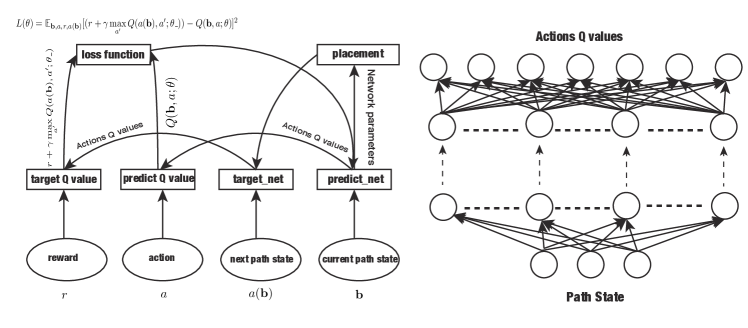
Figure 2: Sketch of the RL architecture used in this work. Left panel shows the relationship between various quantities and functions defining the RL framework. The ‘predict_net’ and ‘target_net’ are two networks having network-parameters $\theta$ and $\theta_{-}$ (see Section II.1 and algorithm 1), which represent the Q-table in the reinforcement learning. In the training process, the network ‘predict_net’ is trained on the fly—it is updated in every training step. The network parameters in ‘target_net’ are updated to that in ‘predict_net’ every $W$ steps by ‘placement’ as explained in the main text. We train the network ‘predict_net’ such that its produced Q-value through the function ‘predict Q value’ matches the reward of the current path state plus the discounted maximal Q-value of actions performing on the next path state, produced by the delayed network ‘target_net’ and the function ‘target Q value’. The ‘loss function’ is defined accordingly. Right panel illustrates the structure of the fully-connected multi-layer neural networks representing the Q-table whose input is the path state and the output is the Q-values corresponding to the different actions.

Our method uses a deep neural network to approximate the Q-table, as $Q^{\star}({\bf b},{a})\approx Q({\bf b},{a};\theta)$, with $\theta$ the network parameters determined in an iterative learning process. To stabilize the nonlinear iteration in learning, we adopt an experience-replay approach Mnih et al. (2015) where the agent’s experiences $({\bf b},a,r)$ are stored in a memory ${\cal M}$ with a capacity $CAP$. We have a network $Q({\bf b},a;\theta)$ trained on-the-fly during the agent exploring the path-state space. As for the training, the inputs and outputs are ${\bf b}$ and $r+\gamma\,{\rm max}_{a^{\prime}}Q(a({\bf b}),a^{\prime};\theta_{-})$ respectively, with ${\bf b}$, $r$, and $a$ drawn randomly from the memory ${\cal M}$, and the network parameter $\theta_{-}$ updated to $\theta$ every $W$ steps.

Given the limitations of quantum computing hardwares presently accessible, we simulate quantum computing on a classical computer and generate reward to train the RL network. In applications to a quantum computer, our RL architecture for automated algorithm design is directly adaptable by collecting reward generated by a quantum adiabatic computer.

II.2 Neural network architecture

In Fig. 2 we show the explicit learning protocol. The left-hand panel of Fig. 2 shows a schematic of our RL framework. We use a two-network setup which is similar to that used in Ref. Mnih et al., 2015. These two networks are labeled ‘target_net’ and ‘predict_net’ in the schematic. The ‘target_net’ uses a previously-learned set of parameters and updates the parameters every $W$ steps; the values of these parameters are directly copied from ‘predict_net’. This will reduce problems such as divergences and oscillations thus making the learning process more stable. The loss function calculates the expectation value of the difference between ‘target Q value’ and ‘predict Q value’ over different batches. The right-hand panel shows the multi-layer fully-connected neural network used to represent the Q-table. The input to this network is the path state obtained at some learning step, while the output are the Q-values corresponding to the actions.

II.3 Details of the state-update policy in the reinforcement learning

For the state-update policy, we used the $\epsilon$ greedy strategy, where the agent selects a random action with total probability $1-\epsilon$, and the action having the maximal Q-value with an additional probability $\epsilon$. We set the $\epsilon=0$ initially and let the agent explore the state space with no preference. The value of $\epsilon$ is increased gradually until a maximum value $90\%$ in the learning process. In this way, we try to maintain a balance between the agent’s current knowledge to maximize reward and possibilities in exploring among other options, which in turn leads to a learning process with better performance.

In order to deal with the continuous state-space, we develop a continuous state-update protocol and combine with the $\epsilon$-greedy method in the following way. In our procedure, we use the $\epsilon$-greedy strategy to choose an action. After choosing the action, the agent sets a probability to accept the action which we calculate from an acceptance probability function $P(e,Tem)=\exp\left(\frac{e}{Tem}\right)$, where

$$e=\frac{Q(a(\mathbf{b}),a;\theta)-Q(\mathbf{b},a;\theta)}{\Delta_{0}}*\Delta,\,\,\,\,\,\,\Delta\in[0,\Delta_{0}],$$ (3)

$Tem$ is a modifiable parameter commonly identified as the “temperature” of the system in the context of simulated annealing methods, The “temperature” is annealed down every agent-exploration step (labeled by $j$), following $Tem_{j}=Tem_{j-1}\times 10^{-C_{R}}$, withe $C_{R}$ the cooling rate. We run cycles of this $\epsilon$-greedy learning process to ensure convergence of the Q-table. At each step of RL exploration, the neural network is trained by varying the $\theta$ parameters to solve an iteration problem,

$$Q({\bf b},a;\theta)=r(a({\bf b}))+\gamma\,{\rm max}_{a^{\prime}}\left[Q(a({\bf b}),a^{\prime};\theta_{-})\right].$$ (4)

The training data is generated from the memory ${\cal M}$ that stores the path-states ${\bf b}$, actions $a$, and the corresponding rewards $r(a({\bf b}))$ that the RL agent has explored. The parameters $\theta_{-}$ are only updated to $\theta$ every $W$ steps ($W$ is set to be $50$ here), to deliberately slow down the iteration process for stabilization purpose. This approach has been used in Ref. Mnih et al., 2015, and follows a standard approach to stabilize nonlinear iteration problems. When the iteration converges, $Q({\bf b},a;\theta)$ satisfies the Bellman equation Bellman (1952).

The effect of $P(e,Tem)$ can be better understood in context of the annealing procedure, which we outline below. At intermediate step $j$ the agent evaluates the action $a_{j}$ on the path state $\mathbf{b}_{j}$, which then defines the path state $\mathbf{b}_{j+1}$ and reward at step $j+1$. At this point we perform the following steps,

• Fix $\Delta_{0}$ to some constant;

• Calculate (3) with values of the parameters as obtained at step $j$;

• Generate a random number $\mu\in[0.0,1.0]$

• If $\mu\leq\exp\left(\frac{e}{Tem}\right)$

  • Accept corresponding action and accept the current value of $\Delta$.

• else choose action $=0$ (corresponding to taking no action).

In the learning process, we store the current path, action taken, reward resulting from action on path state and the corresponding next path state.

When the reward reaches a threshold of $99.9\%$—a maximal reward is $1$ in our notation, as it resembles the success probability of the RL-designed adiabatic algorithm, the value of $\varepsilon_{max}$ is set to $1$, and the agent then uses the network to choose action. In exploring the Hamiltonian path-state space, as the iteration step increases, it gets more frequent for the agent to find a path that gives a higher success probability.

After the Q-table converges, we let the agent update the path-state ${\bf b}$ until it stabilizes, according to the $\epsilon$-greedy policy with $\epsilon$ increased from $90\%$ to $100\%$ slowly with fixed annealing temperature and neural network parameters

Figure 3: Performance of RL-designed quantum adiabatic algorithm in success probability for Grover search. The success probability is obtained by taking the square of wave-function overlap of the dynamical quantum state with search-target state. Results from adiabatic algorithms using a linear and a tailored nonlinear path Roland and Cerf (2002) are shown for comparison. The total adiabatic time are chosen to be $T=22.0,31.1,62.2,124.5,248.9,497.8$ for qubit number $n=1,2,4,6,8,10$, respectively, following the $\sqrt{N}=\sqrt{2^{n}}$ scaling. Given this choice of scaling, an eventual success probability close to $1$ by both of the non-linear and the RL-designed algorithms implies that they both exhibit quadratic quantum speedup because otherwise the success probability would dropdown with increasing qubit number. Comparing the RL-designed and non-linear algorithms quantitatively, it takes less amount of time for RL-designed algorithm to converge to the searching target than the non-linear algorithm.

III Performance on Grover search

III.1 Learning of easy Grover search

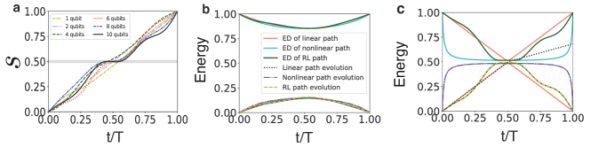
Figure 4: Energy evolution from the RL-designed adiabatic path for Grover search. (a) shows the RL-designed path. The adiabatic time is chosen the same way as in Fig. 2 (see the main text). (b) and (c) show the energy spectrum for the ground and first excited states with $1$ and $10$ qubits, respectively. The energy spectra of the instantaneous Hamiltonian are obtained by exact diagonalization (ED), shown by solid lines in (b, c). The plot in (c) shares the same legend as in (b). The energy expectation values of the dynamical state following different Hamiltonian paths are shown by dashed lines. It is evident from (${\bf c}$) that the RL-designed path is distinct from both of the linear and the nonlinear paths.

In application of our RL approach to automated adiabatic algorithm design, we first show its performance on Grover search compared to known quantum algorithms. This search problem is to find an element in an array of length $N$ as an input to a black-box function that produces a particular output value. This classical problem can be encoded as searching in the Hilbert space of $n=\log_{2}N$ qubits for a target quantum state. These qubits are labeled by $q$ in the following. A circuit-based quantum algorithm was firstly designed by Grover, which shows a quadratic quantum speedup over classical computing Grover (1996). In adiabatic quantum computing, the Hamiltonians in Eq. (1) for Grover search are $H_{B}=\mathbb{1}-|\psi_{0}\rangle\langle\psi_{0}|$, and $H_{P}=\mathbb{1}-|m\rangle\langle m|$, where $|m\rangle$ is a product state in Pauli-$Z$ basis that encodes the search target, and $|\psi_{0}\rangle$ is a product state in the Pauli-$X$ basis with all $n$ eigenvalues equal to $1$. The symbols $X$, $Y$, and $Z$ refer to Pauli matrices in this work. A linear choice of $s(t/T)$ (${\bf b}=0$ in our notation), does not exhibit the quadratic speedup. It was later pointed out in Ref. Roland and Cerf, 2002 that the quantum speedup is restored with a tailored nonlinear path choice of $s(t/T)$.

In the Grover search problem, different problem instances correspond to different choices for the $|m\rangle$ states, which are all connected to each other by a unitary transformation which keeps $H_{B}$ invariant. The reward RL-agent collects in the training process is thus exactly equivalent for different problem instances, which means averaging over $PI$ is unnecessary for the Grover search. Fig. 3 shows results of the RL-designed adiabatic Grover search algorithm. In our RL design for adiabatic quantum algorithm, we scale up the adiabatic time $T$ as $T\propto\sqrt{N}$ to benchmark against the best-known Grover search algorithm. Then as expected, the linear adiabatic algorithm leads to a success probability completely unsatisfactory at large $N$. We find that both the nonlinear Roland and Cerf (2002) and the RL-designed adiabatic algorithms produce success probabilities very close to $1$ (larger than $99.9\%$). At large $N\geq 2^{4}$, the RL-designed algorithm outperforms the nonlinear one.

In Fig. 3, a quantitative comparison shows that the required adiabatic time $T$ to reach a fixed success probability is shorter from the RL-designed algorithm than the analytically constructed non-linear algorithm. We want to emphasize here that in Fig. 3 we scale up the total adiabatic time according to the $\sqrt{N}=\sqrt{2^{n}}$ scaling. Having an eventual success probability close to $1$ implies the the computational complexity of the RL-designed adiabatic algorithm follows the $\sqrt{N}$ scaling, because otherwise the success probability would significantly decrease as we increase the qubit number from $1$ to $10$. The $\sqrt{N}$ scaling is already known to be optimal for Grover search Farhi and Gutmann (1998).

It is worth remarking that the choice of $H_{B}$ is made here for comparison purposes, as the nonlinear path to achieve the quadratic speedup is only analytically available with that specific Hamiltonian choice Roland and Cerf (2002). For physical realization of $H_{B}$, which can be rewritten as $H_{B}=\mathbb{1}-\otimes_{q}[1+X_{q}]/2$, it is experimentally challenging to construct this Hamiltonian with quantum annealing devices. A more suitable choice for $H_{B}$ in that regard is $\sum_{q}[\mathbb{1}-X_{q}]/2$, for which the analytically obtained nonlinear path Roland and Cerf (2002) is then no longer applicable, but our RL design still produces high-performance adiabatic algorithms. A common feature of the RL-learned path for $s(t/T)$ is that there is a relatively flat region around $s=0.5$ where the energy gap is minimal. This flat region has a tendency to grow as we increase $N$ (Fig. 4(a)).

III.2 Instantaneous energy spectrum for the easy Grover search

In this section, we show the resultant instantaneous energy spectrum corresponding to the RL-designed algorithm for the easy-way Grover search.

The instantaneous energy following the RL-designed algorithm lies on the time-dependent ground state for both small and large number of qubits (Fig. 4(b,c)). The energy deviation is much smaller than the linear algorithm, and is very close to the tailored nonlinear algorithm. Therefore the RL-design approach indeed automatically reveals a quantum adiabatic algorithm as efficient as the improved nonlinear algorithm for Grover search Roland and Cerf (2002).

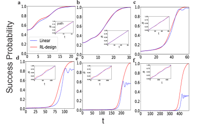
Figure 5: Success probabilities for the hard Grover problem for different number of qubits. Comparison is between a linear protocol and our RL-designed protocol. The nonlinear protocol is not applicable here. The qubit numbers are, from top to bottom, left to right, $n=1,2,4,6,8,10$ for the the adiabatic evolution times $T=22.0,31.1,62.2,124.5,248.9,497.8$.

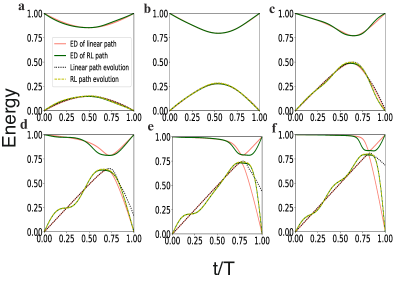
Figure 6: Energy spectrum for the hard Grover problem for different number of qubits. The qubit numbers $n$ and adiabatic evolution times $T$ are the same as those given in the caption of Fig. 5. The expectation value of the instantaneous Hamiltonian by ED and the dynamical state following linear and RL-designed Hamiltonian path are shown by ‘solid’ and ‘dashed’ line. We do not show the nonlinear results as they are not applicable here.

III.3 Hard Grover search

In learning the adiabatic algorithm of the Grover search, we choose the analytical-solvable Hamiltonian as in Ref. Roland and Cerf, 2002 for comparison purpose, where the quantum dynamics during the adiabatic procedure corresponds to an effective two-level system.

We thus denote this as the “easy” Grover problem. Considering physical realization, a suitable choice for the encoding Hamiltonian $H_{B}$ is

$$H_{B}=\sum_{q}[\mathbb{1}-X_{q}]/2$$ (5)

We denote this the “hard” Grover problem, for which the analytically obtained nonlinear path Roland and Cerf (2002) does not carry over Jarret et al. (2018); Slutskii et al. (2019). We stress here that our RL approach still produces an adiabatic algorithm with high success probability. In this regard, our RL approach is more generic, and is particularly useful considering the present limitations of quantum hardwares.

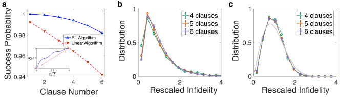
Figure 7: Performance of reinforcement learning (RL) designed algorithm on 3-SAT problem. In (a), we show the comparison of the RL-designed and linear algorithms in the averaged success probability of solving random 3-SAT problems. The success probability is defined by projecting the final state of the adiabatic quantum evolution onto the correct solutions. (b) and (c) show the distribution of the infidelity for the RL-designed and linear algorithms, respectively. The statistics is collected from solving $10^{5}$ random 3-SAT problem instances using the corresponding quantum algorithms. The error bar represents the statistical error according to the bootstrap method. The infidelity is rescaled by taking its average as a unit. The infidelity distribution from the linear algorithm shown in (${\bf c}$) empirically resembles a Wigner-Dyson type (illustrated by the ‘grey’ solid line), whereas the distribution from the RL algorithm in (${\bf b}$) deviates from that. In this plot we choose the adiabatic time $T=6$, and the total bit number $N_{b}=10$.

In Fig. 5, we compare results obtained from the linear protocol with those obtained from the RL-learned protocol for the hard Grover problem. We show the success probabilities as obtained from the linear and RL designed path for different numbers of qubits. Similarly to our results in Fig. 3, the success probability is calculated by taking the square of wave function overlap between the dynamical and targeted ground state. Again, at large $N$ the linear search algorithm fails to find the targeted state (the evolution time follows the scaling of $T\propto\sqrt{N}$), while the RL-designed algorithm still produces an adiabatic algorithm with high performance. The comparison to the nonlinear path is not shown here simply because for the hard Grover search Hamiltonian used here, the nonlinear path is not analytically available.

In Fig. 6 we plot the energy spectrum of the instantaneous Hamiltonian of the hard Grover problem for different numbers of qubits. The behavior of the ground and first excited states of the hard Grover problem is markedly different from those of the easy Grover case (Fig. 4). As can be seen from the plots, the linear protocol apparently starts to fail for $n=6$.

IV Performance on 3-SAT

We then apply the RL approach to the more complicated 3-SAT problem. Given a total number of $N_{b}$ boolean bits (labeled by $q$), the problem is to find a boolean sequence $z_{q}$ to satisfy $C=C_{1}\land C_{2}\land C_{3}\land C_{4}\land\dots$ with each $C_{i}$ a clause containing three boolean bits, say $q_{i,k=1,2,3}$. The total clause number will be denoted as $N_{C}$. The satisfiability condition of each clause $C_{i}$ can be written into a truth table ${\bf z}_{i\alpha}=\{z^{(1)},z^{(2)},z^{(3)}\}$ such that the binary sequence $\{z^{(1)},z^{(2)},z^{(3)}\}$ belongs to this table if and only if $C_{i}$ is satisfied. We use $\alpha$ to label all possibilities to satisfy the clause $C_{i}$. To solve this problem with quantum adiabatic algorithm, we need to introduce $N_{b}$ qubits, which are then also labeled by $q$. The corresponding qubit states are $|z_{1}\rangle\otimes|z_{2}\rangle\otimes\ldots\otimes|z_{N_{b}}\rangle$. Introducing a compact notation $|{\bf q}_{i};{\bf z}_{i\alpha}\rangle$ for the qubits, ${q}_{i,1}$, $q_{i,2}$, and $q_{i,3}$, in the quantum state $|z^{(1)}\rangle\otimes|z^{(2)}\rangle\otimes|z^{(3)}\rangle$, the classical 3-SAT problem is formally encoded into a quantum ground state problem with a Hamiltonian

$$\textstyle H_{P}^{\rm SAT}=-\sum_{i=1}^{N_{C}}\sum_{\alpha}|{\bf q}_{i};{\bf z}_{i\alpha}\rangle\langle{\bf q}_{i};{\bf z}_{i\alpha}|.$$ (6)

A solution to the 3-SAT problem corresponds to a ground state of $H_{p}^{\rm SAT}$ with energy $-N_{C}$. Different 3-SAT problem instances correspond to different choices of clause ${\bf q}_{i}$ and truth table ${\bf z}_{i\alpha}$. The initial quantum state and Hamiltonian $H_{B}$ are set to be $|\psi_{0}\rangle$ and $H_{B}=\sum_{q}[\mathbb{1}-X_{q}]/2$, respectively, where $|\psi_{0}\rangle$ is the same initial state as in the Grover search problem. In our RL approach to design 3-SAT quantum algorithm, the reward RL-agent collects is generated by randomly sampling ${\bf q}_{i}$ and ${\bf z}_{i\alpha}$ (see Appendix B), to make the learned algorithm generically applicable.

In Fig. 7, we show the performance of the RL-designed algorithm and compare with the linear algorithm. We put the RL-agent to work on a $10$-bit 3-SAT problem. The RL-designed algorithm is obtained by training with clause number $N_{C}=3$ only, where the stepwise reward is obtained by averaging over $100$ random problem instances. We then test the RL algorithm on random 3-SAT problem instances that contain one-to-six clauses. The tested success probability in Fig. 7(a) is obtained by averaging over $10^{5}$ random problem instances. It is evident that the RL-designed algorithm outperforms the linear algorithm with higher success probability. Its advantage becomes more significant in a systematic fashion as the clause number is increased, although the RL algorithm is trained on 3-SAT problems with clause number $N_{C}=3$ only. This implies the emergent transferability of the RL-designed algorithm. The success over different clause numbers implies that this RL-learning approach has seized the intrinsic ingredients to optimize the adiabatic quantum algorithm because otherwise the RL-designed algorithm would not be transferable.

Besides the quantitative improvement in the RL-designed over the linear algorithm, we also emphasize that the outcome of the RL algorithm is qualitatively distinct in the resultant fidelity. In Fig. 7(b, c), we show the distribution of the infidelity obtained from $10^{5}$ random 3-SAT problem instances. The statistics is taken for different clause number separately. The infidelity is rescaled by taking its average as a unit. The distributions of this rescaled infidelity for different clause numbers are found to collapse onto a universal function, for both the RL (Fig. 7(b)) and linear (Fig. 7(c)) algorithms. It appears that infidelity distribution from the linear algorithm is close to a Wigner-Dyson (WD) distribution—the numerically obtained statistical second moment of the infidelity agrees with the WD prediction within $10\%$ difference. To the contrast, the second moment of the infidelity from the RL algorithm deviates from the WD prediction, meaning the infidelity distribution for the RL algorithm is qualitatively distinctive from the linear case. The physical implication of such qualitative difference in the infidelity distribution is left for future study.

Figure 8: Performance of linear and machine learning designed quantum adiabatic algorithms applied to Grover search with different number of qubits. In this plot, the reinforcement learning (RL) designed schedule $s(t/T)$ is obtained by training on the problem with qubit number $n=10$, and then applied to problems having larger number of qubits, $11$ to $16$, by a simple rescaling $T\propto\sqrt{2^{n}}$. The RL-designed adiabatic algorithm systematically out-performs the linear one.

V Scalability of the reinforcement learning in quantum adiabatic algorithm design on Grover Search

In Fig. 8 we show the results of applying a schedule learned on a $10$-qubit easy Grover search problem to $n$-qubit problems with $n>10$. For the linear algorithm, the schedule is $s(t/T)=t/T$, and $T$ scales according to $\sqrt{2^{n}}$ as we increase the qubit number in Fig. 8. For the RL-designed algorithm, the schedule $s(t/T)$ is obtained by a training process on a problem with qubit number $n=10$, and then the schedule is applied to problems having larger number of qubits ($n=11,\ldots,16$), following the same rescaling $T\propto\sqrt{2^{n}}$ as the linear case. While the fidelity decreases as we increase the qubit number, it is evident that the RL-designed algorithm systematically out-performs the linear algorithm despite the simple rescaling applied. The comparison in the infidelity is explicitly given in Fig. 9.

To further demonstrate the scalability of the RL-learning, we provide the infidelity of the RL-designed algorithm trained on Grover search with qubit number $n$, and then applied successively on a problem with $n+1$ (see Fig. 9). We use the number of training steps to quantify the resources spent on the RL-learning. Assuming access to an actual quantum computer, the number of training steps multiplied by the parameter $MI$ (see Section II.1 and Table 1) would be equal to the number of running times of the quantum computer.

We emphasize here that the number of training steps for different qubit number $n$ is fixed (see parameters of annealing protocol iteration $L_{SA}$ and path state iteration $L_{PS}$ in Table 1). The resultant infidelity in this iterative procedure remains close to $1\%$. This further implies the schedule trained on relatively smaller-size problems has a rather large degree of transferability.

In order to explicitly show that the reinforcement learning is helpful in obtaining a new schedule from a prior guess as we alter the problem, we provide the infidelity during the training process in Fig. 10. We take the qubit number $n=11$, and compare two cases with and without pre-knowledge of the schedule. In Fig. 10 (a), the training process starts from a trivial linear schedule $s(t/T)=t/T$, i.e., no pre-knowledge given, whereas in Fig. 10 (b), the iteration starts from a Q-table already obtained through training on the problem with $n=10$, i.e., with pre-knowledge. It is evident that the reinforcement learning is indeed substantially helpful in quickly finding a new schedule from a prior guess even when the problem is altered—here the qubit number is changed from $n=10$ to $11$. With pre-knowledge, our reinforcement learning is able to find a proper schedule with three times smaller of iteration steps.

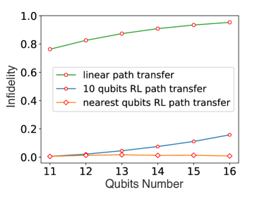
Figure 9: Transferability of reinforcement learning designed schedules for Grover search. The ‘green’ line shows the resultant infidelity from the linear schedule $s(t/T)=t/T$ as a comparison. The ‘blue’ line shows the infidelity following the schedule that is obtained by training on the problem with qubit number $n=10$. The ‘orange’ line corresponds to the schedules obtained by training on the problem with qubit number $n$ under a fixed number of training steps (see parameters of annealing protocol iteration $L_{SA}$ and path state iteration $L_{PS}$ in Table 1 ) and then applied to the problem with qubit number $n+1$. In this plot, the total adiabatic time $T$ is chosen to scale with the qubit number as $T\propto\sqrt{2^{n}}$.

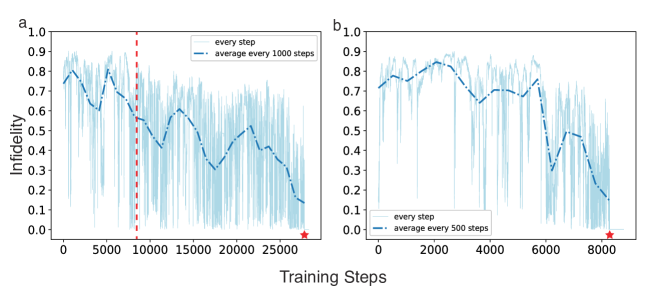
Figure 10: Stepwise infidelity during the reinforcement learning process (a) without and (b) with pre-knowledge. The results in this plot correspond to easy Grover search problem with qubit number $n=11$ In (a), the training process starts from a trivial linear schedule. In (b), the process starts from a schedule obtained for Grover search with qubit number $n=10$ (rescaled according to $\sqrt{2^{n}}$). In both cases, the infidelity does not asymptotically converge to $0$ during the training process, but instead the chance for the learning agent to find a low-infidelity schedule is getting more frequent with more iteration steps. The red star in both plots marks the point where the performance reaches the threshold and $\epsilon_{max}$ in the $\epsilon$-greedy policy is set to be $1$. Comparing (a) and (b), at an iteration step around $8000$ (at the position of ‘red’ vertical dashed line in (a) and the end of (b), the chance for the learning agent with pre-knowledge to find a low-infidelity schedule is substantially more frequent than that without pre-knowledge. The averaged infidelity in (b) drops down with much less iteration steps than in (a).

VI Conclusion

In this work we report a reinforcement-learning-based approach for automated quantum adiabatic algorithm design. Our devised approach is directly applicable to problems with solutions easy-to-verify such as searching, factorization, and NP-complete problems. Through numerical simulations, we show that the RL approach automatically finds an adiabatic algorithm for Grover search with quadratic speedup. In the application to the 3-SAT problems, we find surprising transferability of the RL-designed algorithm which suggests the algorithm trained on relatively-smaller size problems is applicable to larger sizes, which is both practically useful and theoretically inspiring in considering the complexity scaling. The performance of our approach can be further improved by introducing additional Hamiltonian terms, which would easily fit into the framework proposed here.

VII Acknowledgement

J.L. acknowledges helpful discussion with Xiuzhe Luo. This work is supported by National Program on Key Basic Research Project of China under Grant No. 2017YFA0304204, National Natural Science Foundation of China under Grants No. 11774067, 11934002, and Natural Science Foundation of Shanghai City (Grant No. 19ZR1471500), Shanghai Municipal Science and Technology Major Project (Grant No.2019SHZDZX04). XL would like to thank Department of Physics at Harvard University for hospitality during the completion of this work. The first two authors J.L. and Z.Y.L. contribute equally to this work.

Appendix

Appendix A pseudo code and parameters of reinforcement learning

For completeness, the pseudo code and the parameters used in our RL architecture for Grover search and 3-SAT problems are shown in algorithm 1 and Table 1.

Algorithm 1 RL architecture for automated adiabatic quantum algorithm design.

1:Initialize “temperature” in simulation annealing $Tem_{0}$; Initialize memory ${\cal M}$; Initialize path state; Initialize predict action-value $Q$ neural network with random weight $\theta$; Initialize target action-value $Q$ neural network with weight $\theta_{-}=\theta$;

2:for  simulation annealing iteration $j=1,L_{SA}$ do

3:   Set “temperature” $Tem_{j}=Tem_{j-1}*10^{-C_{R}}$

4:   for path state iteration $i=1,L_{PS}$ do

5:      With probability $1-\epsilon$ select a random action $a_{i}$,and with probability $\epsilon$ select $a_{i}=argmax_{a}Q(\mathbf{b}_{i},a;\theta)$.

6:      Accept and execute action $a_{i}$ on $\mathbf{b}_{i}$ with probability $P(e,Tem_{j})$

7:      Get the next path state $a_{i}(\mathbf{b}_{i})$ and the reward $r_{i}$ by averaging the performance of $MI$ instances. (The number of training steps multiplied by $MI$ is then equal to the number of running times of the quantum computer, which is simulated in our work. The number of training steps is thus a valid measure of computation resources spent on the RL-learning.)

8:      Store transition $(\mathbf{b}_{i},a_{i},r_{i},a_{i}(\mathbf{b}_{i}))$ in memory ${\cal M}$

9:      Sample a batch of transitions$(\mathbf{b},a,r,a(\mathbf{b}))$ from memory randomly

10:      Perform a stochastic gradient descent on the loss function $L(\theta)=\mathbb{E}_{\mathbf{b},a,r,a(\mathbf{b})}[(r+\gamma\max_{a^{\prime}}Q(a(\mathbf{b}),a^{\prime};\theta_{-}))-Q(\mathbf{b},a;\theta)]^{2}$ with respect to the predict network parameter $\theta$

11:      Increase $\epsilon$ with single step increment. Here set upper bound of $\epsilon$ value $\epsilon_{max}$

12:      Every $W$ steps, set $\theta_{-}=\theta$

13:      if $r_{i}\geq threshold$ then

14:         Keep on path state updating iteration without training and set $\epsilon_{max}$ to be $1$

15:      end if

16:   end for

17:end for

18:path state

Table 1: Parameter list in the reinforcement learning

	Easy/Hard Grover Search	3-SAT
Neural-network layer number	2	3
Neural-network hidden-layer neurons	20	12
Neural-network learning rate	0.01	0.01
Neural-network activation function	relu	relu
Training bath size	32	32
Reward discount factor, $\gamma$	0.9	0.9
Memory capacity, CAP	500	1000
Maximal $\varepsilon$-value in $\epsilon$-greedy policy, $\epsilon_{max}$	0.9	0.9
Single-step increment of $\epsilon$	0.01	0.01
Target-Net refreshing parameter, $W$	50	50
Cooling rate in annealing protocol, $C_{R}$	0.1	0.1
Initial “temperature” in annealing, $Tem_{0}$	10	10
Cutoff, $C$	6	6
Maximal update per step, $\Delta_{0}$	0.1	0.1
Problem instance averaging number, MI	1	100
Annealing protocol iteration, $L_{SA}$	80	80
Path state iteration, $L_{PS}$	1000	1000

Appendix B Sampling of 3-SAT problem instances

Given a total number $N_{b}$ of boolean bits $z_{q}$, different 3-SAT problem instances correspond to different choices of three-bit combinations ${\bf q}_{i}$ in each clause $C_{i}$, and different choices of the truth table of each clause defined to be ${\bf z}_{i\alpha}=(z^{(1)},z^{(2)},z^{(3)})$ in the main text. Since we aim at a quantum adiabatic algorithm generically applicable, we randomly sample the problem instances $\{{\bf q}_{i},{\bf z}_{i}\}$ according to the definition of 3-SAT problem. It is worth noting here that the choice for the truth table is not completely random, and that for one clause in the 3-SAT problem, there are eight possibilities of choosing the truth table corresponding to the eight possibilities of constructing the clause. The size of the sampling space grows polynomially with $N_{b}$ and exponentially with $N_{C}$.

References

- Preskill (2012) J. Preskill, arXiv preprint arXiv:1203.5813 (2012).
- Harrow and Montanaro (2017) A. W. Harrow and A. Montanaro, Nature 549, 203 (2017).
- Lund et al. (2017) A. Lund, M. J. Bremner, and T. Ralph, npj Quantum Information 3, 15 (2017).
- Bloch (2018) I. Bloch, Nature Physics 14, 1159 (2018).
- Arute et al. (2019) F. Arute, K. Arya, R. Babbush, D. Bacon, J. C. Bardin, R. Barends, R. Biswas, S. Boixo, F. G. Brandao, D. A. Buell, et al., Nature 574, 505 (2019).
- Shor (1999) P. W. Shor, SIAM review 41, 303 (1999).
- Nielsen and Chuang (2002) M. A. Nielsen and I. Chuang, Quantum computation and quantum information (2002).
- Farhi et al. (2001) E. Farhi, J. Goldstone, S. Gutmann, J. Lapan, A. Lundgren, and D. Preda, Science 292, 472 (2001), ISSN 0036-8075, eprint http://science.sciencemag.org/content/292/5516/472.full.pdf.
- Albash and Lidar (2018) T. Albash and D. A. Lidar, Rev. Mod. Phys. 90, 015002 (2018).
- Devoret and Schoelkopf (2013) M. H. Devoret and R. J. Schoelkopf, Science 339, 1169 (2013).
- Otterbach et al. (2017) J. Otterbach, R. Manenti, N. Alidoust, A. Bestwick, M. Block, B. Bloom, S. Caldwell, N. Didier, E. S. Fried, S. Hong, et al., arXiv preprint arXiv:1712.05771 (2017).
- (12) Ibm q experience, https://quantumexperience.ng.bluemix.net.
- King et al. (2018) A. D. King, J. Carrasquilla, J. Raymond, I. Ozfidan, E. Andriyash, A. Berkley, M. Reis, T. Lanting, R. Harris, F. Altomare, et al., Nature 560, 456 (2018).
- Neill et al. (2018) C. Neill, P. Roushan, K. Kechedzhi, S. Boixo, S. Isakov, V. Smelyanskiy, A. Megrant, B. Chiaro, A. Dunsworth, K. Arya, et al., Science 360, 195 (2018).
- Gong et al. (2018) M. Gong, M.-C. Chen, Y. Zheng, S. Wang, C. Zha, H. Deng, Z. Yan, H. Rong, Y. Wu, S. Li, et al., arXiv preprint arXiv:1811.02292 (2018).
- Flamini et al. (2018) F. Flamini, N. Spagnolo, and F. Sciarrino, Reports on Progress in Physics 82, 016001 (2018).
- Brod et al. (2019) D. J. Brod, E. F. Galvão, A. Crespi, R. Osellame, N. Spagnolo, and F. Sciarrino, Advanced Photonics 1, 034001 (2019).
- Wang et al. (2019) H. Wang, J. Qin, X. Ding, M.-C. Chen, S. Chen, X. You, Y.-M. He, X. Jiang, L. You, Z. Wang, et al., Physical review letters 123, 250503 (2019).
- Brown et al. (2016) K. R. Brown, J. Kim, and C. Monroe, npj Quantum Information 2, 16034 (2016).
- Bernien et al. (2017) H. Bernien, S. Schwartz, A. Keesling, H. Levine, A. Omran, H. Pichler, S. Choi, A. S. Zibrov, M. Endres, M. Greiner, et al., Nature 551, 579 (2017).
- Wu et al. (2018) T.-Y. Wu, A. Kumar, F. G. Mejia, and D. S. Weiss, arXiv preprint arXiv:1809.09197 (2018).
- Van Dam et al. (2001) W. Van Dam, M. Mosca, and U. Vazirani, in Foundations of Computer Science, 2001. Proceedings. 42nd IEEE Symposium on (IEEE, 2001), pp. 279–287.
- Aharonov et al. (2008) D. Aharonov, W. Van Dam, J. Kempe, Z. Landau, S. Lloyd, and O. Regev, SIAM review 50, 755 (2008).
- Yu et al. (2018) H. Yu, Y. Huang, and B. Wu, Chinese Physics Letters 35, 110303 (2018).
- Roland and Cerf (2002) J. Roland and N. J. Cerf, Phys. Rev. A 65, 042308 (2002).
- Preskill (2018) J. Preskill, Quantum 2, 79 (2018), ISSN 2521-327X.
- Bukov et al. (2018) M. Bukov, A. G. R. Day, D. Sels, P. Weinberg, A. Polkovnikov, and P. Mehta, Phys. Rev. X 8, 031086 (2018).
- Berry (2009) M. V. Berry, Journal of Physics A: Mathematical and Theoretical 42, 365303 (2009).
- Chen et al. (2010) X. Chen, I. Lizuain, A. Ruschhaupt, D. Guéry-Odelin, and J. Muga, Physical review letters 105, 123003 (2010).
- Yang et al. (2018) X.-C. Yang, M.-H. Yung, and X. Wang, Phys. Rev. A 97, 042324 (2018).
- Niu et al. (2018) M. Y. Niu, S. Boixo, V. Smelyanskiy, and H. Neven, arXiv preprint arXiv:1803.01857 (2018).
- (32) D-wave quantum computer, https://www.dwavesys.com.
- Silver et al. (2017) D. Silver, J. Schrittwieser, K. Simonyan, I. Antonoglou, A. Huang, A. Guez, T. Hubert, L. Baker, M. Lai, A. Bolton, et al., Nature 550, 354 (2017).
- Bellman (1952) R. Bellman, Proceedings of the National Academy of Sciences 38, 716 (1952).
- Mnih et al. (2015) V. Mnih, K. Kavukcuoglu, D. Silver, A. A. Rusu, J. Veness, M. G. Bellemare, A. Graves, M. Riedmiller, A. K. Fidjeland, G. Ostrovski, et al., Nature 518, 529 (2015), ISSN 00280836.
- Grover (1996) L. K. Grover, in Proceedings of the twenty-eighth annual ACM symposium on Theory of computing (ACM, 1996), pp. 212–219.
- Farhi and Gutmann (1998) E. Farhi and S. Gutmann, Phys. Rev. A 57, 2403 (1998).
- Jarret et al. (2018) M. Jarret, B. Lackey, A. Liu, and K. Wan, arXiv e-prints arXiv:1810.04686 (2018), eprint 1810.04686.
- Slutskii et al. (2019) M. Slutskii, T. Albash, L. Barash, and I. Hen, arXiv e-prints arXiv:1904.04420 (2019), eprint 1904.04420.