Thermodynamics of delta-chain with ferro- and antiferromagnetic interactions

Abstract

Motivated by a novel cyclic compound $Fe_{10}Gd_{10}$ with record ground state spin in which the arrangement of magnetic ions with $s=\frac{5}{2}$ and $s=\frac{7}{2}$ corresponds to a saw-tooth chain we investigate the thermodynamics of the delta-chain with competing ferro- and antiferromagnetic interactions. We study both classical and quantum versions of the model. The classical model is exactly solved and quantum effects are studied using full diagonalization and a finite temperature Lanczos technique for finite delta-chains as well as modified spin wave theory. It is shown that the main features of the magnetic susceptibility of the quantum spin delta chain are correctly described by the classical spin model, while quantum effects significantly change the low-temperature behavior of the specific heat. The relation of the obtained results to the $Fe_{10}Gd_{10}$ system is discussed.

I Introduction

Low-dimensional quantum magnets on geometrically frustrated lattices have attracted much interest in last years diep ; mila ; qm . An important class of such systems includes lattices consisting of triangles. An interesting and typical example of these objects is the delta or the sawtooth Heisenberg model consisting of a linear chain of triangles as shown in Fig. 1. The Hamiltonian of this model has the form:

$$H=J_{1}\sum_{i=1}^{N}\mathbf{\sigma}_{i}\cdot(\mathbf{S}_{i}+\mathbf{S}_{i+1})+J_{2}\sum_{i=1}^{N}\mathbf{S}_{i}\cdot\mathbf{S}_{i+1}$$ (1)

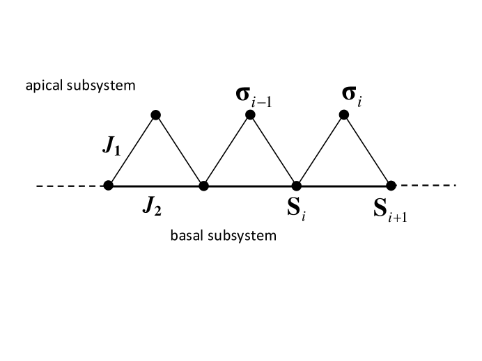
Figure 1: The delta-chain model.

The interaction $J_{1}$ acts between the apical ($\mathbf{\sigma}_{i}$) and the basal ($\mathbf{S}_{i}$) spins, while $J_{2}$ is the interaction between neighboring basal spins. A direct interaction between the apical spins is absent. The quantum $s=\frac{1}{2}$ delta-chain with antiferromagnetic (AF) exchange interactions $J_{1}$ and $J_{2}$ ($J_{1},J_{2}>0$) has been studied extensively and it exhibits a variety of peculiar properties flat ; Zhit ; Schmidt ; Honecker ; Derzhko2004 . At the same time the $s=\frac{1}{2}$ delta-chain with ferromagnetic $J_{2}$ and antiferromagnetic $J_{1}$ interaction (F-AF delta-chain) is very interesting as well and has unusual properties. In particular, the ground state of this model is ferromagnetic for $a=\frac{J_{2}}{\left|J_{1}\right|}<\frac{1}{2}$ and as it is believed Tonegawa that it is ferrimagnetic for $a>\frac{1}{2}$. The critical point $a=\frac{1}{2}$ is the transition point between these two ground state phases. The $s=\frac{1}{2}$ F-AF delta-chain at the critical point $a=\frac{1}{2}$ has been studied in Ref. KDNDR . It is an example of a quantum system with a flat excitation band flat ; Flach , that provides the possibility to find several rigorous results for the quantum many-body system at hand. Thus, it was shown KDNDR that the ground state at the critical point consists of localized multi-magnon complexes, and it is macroscopically degenerate. An additional motivation for the study of this model is the existence of real compounds, malonate-bridged copper complexes Inagaki ; Tonegawa ; ruiz ; Kaburagi , which are described by this model.

The $s=\frac{1}{2}$ F-AF model can be extended to the delta-chain composed of two types of spins ($\mathbf{\sigma}_{i},\mathbf{S}_{i}$) characterized by the spin quantum numbers $S_{a}$ and $S_{b}$ of the apical and basal spins, respectively. The ground state of this model is ferromagnetic for $a=\frac{J_{2}}{\left|J_{1}\right|}<\frac{S_{a}}{2S_{b}}$ and non-collinear ferrimagnetic for $a>\frac{S_{a}}{2S_{b}}$. The critical point between these phases is $a_{c}=\frac{S_{a}}{2S_{b}}$. The ground state at the critical point consists of exact multi-magnon states as well as for the $s=\frac{1}{2}$ model and has similar macroscopic degeneracy KDNDR .

Recently a mixed $3d/4f$ cyclic coordination cluster
$[Fe_{10}Gd_{10}(Me-tea)_{10}(Me-teaH)_{10}(NO_{3})_{10}]20MeCN$ (i.e. $Fe_{10}Gd_{10}$) has been synthesized and studied S60 . This cluster consists of $10+10$ alternating gadolinium and iron ions and its spin arrangement corresponds to the delta chain with $Gd$ and $Fe$ ions as the apical and basal spins correspondingly. As it was established in Ref. S60 the exchange interaction between $Fe$ ions is antiferromagnetic ($J_{2}=0.65K$) and the interaction between $Fe$ and $Gd$ is ferromagnetic ($J_{1}=-1.0K$). The spin values of $Fe$ and $Gd$ ions are $S=\frac{5}{2}$ for $Fe^{III}$ and $S=\frac{7}{2}$ for $Gd^{II}$. The ground state spin of this cluster is $S=60$ which is one of the largest spin of a single molecule. This molecule is a finite-size realization of the F-AF delta-chain with $S_{a}=\frac{7}{2}$ and $S_{b}=\frac{5}{2}$. Remarkably, according to the estimate of the values of $J_{1}$ and $J_{2}$ in Ref. S60 the frustration parameter is $a=0.65$, i.e. it is very close to the critical value of $a_{c}=0.7$. Therefore, this molecule, although it is not directly at the critical point and located in the F phase, has properties which are strongly influenced by the nearby quantum critical point. Because the spin quantum numbers for $Fe$ and $Gd$ ions are rather large it seems that the classical approximation for ($S_{a},S_{b}$) F-AF delta-chain is justified, except at very low temperatures when quantum fluctuations can substantially change the properties of the system.

To obtain the classical version of Hamiltonian (1) we set $\sigma_{i}=S_{a}\vec{n}_{i}$ and $S_{i}=S_{b}\vec{n}_{i}$, where $\vec{n}_{i}$ is the unit vector at the i-th site. Taking the limit of infinite $S_{a}$ and $S_{b}$ with a finite ratio $\frac{S_{a}}{S_{b}}$ we arrive at the Hamiltonian of the classical delta chain

$$H=-\sum_{i=1}^{2N}\vec{n}_{i}\cdot\vec{n}_{i+1}+\alpha\sum_{i=1}^{N}\vec{n}_{2i-1}\cdot\vec{n}_{2i+1},$$ (2)

where $N$ is the number of triangles. In (2) we take the apical-basal interaction as $-1$ and the basal-basal interaction $\alpha$ as

$$\alpha=\frac{J_{2}S_{b}}{\left|J_{1}\right|S_{a}}=a\frac{S_{b}}{S_{a}}$$ (3)

which is the frustration parameter of the model.

The ground state phase diagram of the classical model consists of a ferromagnetic phase at $a<\frac{S_{a}}{2S_{b}}$ ($\alpha<\frac{1}{2}$) and a ferrimagnetic one at $a>\frac{S_{a}}{2S_{b}}$ ($\alpha>\frac{1}{2}$). Remarkably, the transition between these phases occurs at the same frustration parameter ($a_{c}=\frac{S_{a}}{2S_{b}}$) as in the quantum model. In terms of $\alpha$ the critical point between the ferromagnetic and ferrimagnetic phases is at $\alpha=\frac{1}{2}$.

One of the goals of this paper is the study of the thermodynamics of the classical version of F-AF Heisenberg model (1), where we put special attention on the parameter region corresponding to $Fe_{10}Gd_{10}$. In what follows we use the normalized temperature

$$t=\frac{T}{\left|J_{1}\right|S_{a}S_{b}}$$ (4)

and the corresponding inverse temperature $\beta=1/t$ to present the thermodynamic properties of model (2). Since the classical ground state exhibits a non-trivial macroscopic degeneracy for $\alpha>\frac{1}{2}$, see Sec. II, we may expect unconventional low-temperature physics especially in the ferromagnetic regime close to the critical point $\alpha_{c}=\frac{1}{2}$.

The effect of quantum fluctuations at low temperatures will be studied by a combination of full exact diagonalization (ED) using J. Schulenburg’s spinpack code spinpack and the finite temperature Lanczos (FTL) technique FTL1 ; FTL2 as well as by the modified spin-wave theory (MSWT) MSWT .

The paper is organized as follows. In Sec. II we describe the ground state of model (2) in different regions of frustration parameter $\alpha$. The partition function, the correlation functions, the specific heat and magnetic susceptibility are calculated in Sec. III. In Sec. IV explicit analytical results for the partition function, the spin correlation functions and the magnetic susceptibility in the low-temperature limit are presented for different regions of the parameter $\alpha$. In Sec. V the scaling law near the critical point $\alpha=\frac{1}{2}$ is established and finite-size effects are estimated. In Sec. VI the quantum effects in the ferromagnetic phase are studied with a particular focus on that value of the frustration parameter $\alpha$ which is relevant for $Fe_{10}Gd_{10}$.

II Ground state

We start our study of model (2) from the determination of the ground state. For this aim it is useful to represent Hamiltonian (2) as a sum over triangle Hamiltonians

$$H=\sum_{i=1}^{N}H_{\Delta}(i),$$ (5)

where the Hamiltonian of a triangle has the form

$$H_{\Delta}(i)=-\vec{n}_{2i-1}\cdot\vec{n}_{2i}-\vec{n}_{2i}\cdot\vec{n}_{2i+1}+\alpha\vec{n}_{2i-1}\cdot\vec{n}_{2i+1}.$$ (6)

To determine the ground state of model (5) we need to find the spin configuration on each triangle which minimizes the classical energy. It turns out that the lowest spin configuration on a triangle is different in the regions $\alpha\leq\frac{1}{2}$ and $\alpha>\frac{1}{2}$. For $\alpha\leq\frac{1}{2}$ the ground state is the trivial ferromagnetic one with all spins on each triangle pointing in the same direction. The global spin configuration of the whole system in this case is obviously ferromagnetic as well.

For $\alpha>\frac{1}{2}$ the lowest classical energy on each triangle is given by the ferrimagnetic configuration, where all spins of triangle $\vec{n}_{1},\vec{n}_{2},\vec{n}_{3}$ lie in the same plane and the spin $\vec{n}_{2}$ forms an equal angle $\theta_{0}$ with spins $\vec{n}_{1}$ and $\vec{n}_{3}$:

$$\vec{n}_{1}\cdot\vec{n}_{2} = \vec{n}_{2}\cdot\vec{n}_{3}=\cos\theta_{0}$$

$$\vec{n}_{1}\cdot\vec{n}_{3} = \cos\left(2\theta_{0}\right)$$

$$\cos\theta_{0} = \frac{1}{2\alpha}.$$ (7)

So, each triangle has the non-zero magnetization $m_{\Delta}=1/\alpha+1$, the direction of which coincides with the apical spin $\vec{n}_{2}$. The spins of the next triangle ($\vec{n}_{3},\vec{n}_{4},\vec{n}_{5}$) also form the ferrimagnetic configuration in the ground state. But in the general case the spins ($\vec{n}_{3},\vec{n}_{4},\vec{n}_{5}$) can lie in any plane, formed by the rotation of the first triangle plane around the spin $\vec{n}_{3}$ by an arbitrary angle Chandra . So, the ground state of the second triangle is degenerate over the angle between planes ($\vec{n}_{1},\vec{n}_{2},\vec{n}_{3}$) and ($\vec{n}_{3},\vec{n}_{4},\vec{n}_{5}$). Then the plane of the third triangle ($\vec{n}_{5},\vec{n}_{6},\vec{n}_{7}$) is rotated by an arbitrary angle around spin $\vec{n}_{5}$, and so on. Hence, the global ground state of the whole system for $\alpha>\frac{1}{2}$ is macroscopically degenerate. Each ground state spin configuration for $\alpha>\frac{1}{2}$ can be represented as a sequence of the points lying on the unit sphere with an equal distance between the neighboring points as shown in Fig. 2.

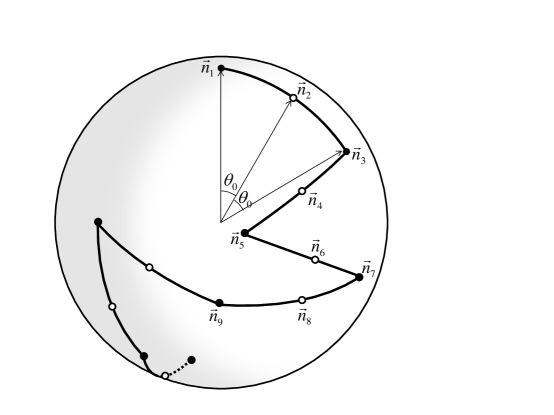
Figure 2: Ground state spin configurations of model (2) for $\alpha>\frac{1}{2}$ as random walk on unit sphere.

III Partition function

The partition function $Z$ of model (2) is

$$Z=(\prod_{i=1}^{2N}\int d\Omega_{i})\exp\left(-\beta H\right),$$ (8)

where $d\Omega_{i}$ is the differential of the solid angle for the $i$-th spin, $d\Omega_{i}=\sin\theta_{i}d\theta_{i}d\varphi_{i}/4\pi$. Using the dual transformation employed in Ref. Harada we choose a local coordinate system connected with the $i$-th spin. The $z_{i}$ axis is parallel to $\vec{n}_{i\text{ }}$and the $y_{i}$ axis is in the plane spanned by $\vec{n}_{i}$ and $\vec{n}_{i+1}$. A new set of the angles $(\theta_{i},\varphi_{i})$ is introduced, where $\theta_{i}$ is the angle between $\vec{n}_{i+1}$ and $\vec{n}_{i}$ and $\varphi_{i}$ is the angle between the components of $\vec{n}_{i+1}$ and $\vec{n}_{i-1}$ projected onto the ($x_{i}$,$y_{i}$) plane. In terms of these variables the Hamiltonian on the triangle (6) becomes

$$H_{\Delta}(i)=-\cos\theta_{2i-1}-\cos\theta_{2i}+\alpha\cos\theta_{2i-1}\cos\theta_{2i}+\alpha\sin\theta_{2i-1}\sin\theta_{2i}\cos\varphi_{2i}.$$ (9)

As follows from the latter equation, the total Hamiltonian (5) does not contain angles $\varphi_{1},\varphi_{3},\varphi_{5}\ldots$, on which the partition function can be integrated. As a result, the partition function reduces to the product of independent multipliers and takes the form

$$Z=\prod_{i=1}^{N}Z_{i}=Z_{\Delta}^{N},$$ (10)

where $Z_{\Delta}$ is ‘the partition function’ of an isolated triangle

$$Z_{\Delta}=\frac{1}{8\pi}\int_{0}^{\pi}\sin\theta_{1}d\theta_{1}\int_{0}^{\pi}\sin\theta_{2}d\theta_{2}\int_{0}^{2\pi}d\varphi_{2}e^{-\beta H_{\Delta}(1)}.$$ (11)

The integral over the angle $\varphi_{2}$ can be carried out analytically:

$$Z_{\Delta}=\frac{1}{4}\int_{0}^{\pi}\sin\theta_{1}d\theta_{1}\int_{0}^{\pi}\sin\theta_{2}d\theta_{2}e^{-\beta H_{1}}I_{0}\left(\beta H_{2}\right),$$ (12)

where

$$H_{1} = -\cos\theta_{1}-\cos\theta_{2}+\alpha\cos\theta_{1}\cos\theta_{2}$$

$$H_{2} = \alpha\sin\theta_{1}\sin\theta_{2}$$ (13)

and

$$I_{0}\left(x\right)=\frac{1}{2\pi}\int_{0}^{2\pi}e^{x\cos\varphi}d\varphi$$ (14)

is the Bessel function of imaginary argument.

Thus, the problem of the calculation of the partition function of model (2) is reduced to the double integral (12). All thermodynamic quantities can be expressed through the corresponding derivatives of the partition function.

III.1 Specific heat

The specific heat can be expressed through the second derivative of the partition function. However, in order to avoid loss of accuracy caused by the numerical derivatives it is convenient to use the following equation for the calculation of the specific heat:

$$C=\beta^{2}\left\langle H_{\Delta}^{2}\right\rangle-\beta^{2}\left\langle H_{\Delta}\right\rangle^{2}.$$ (15)

Here $\left\langle H_{\Delta}\right\rangle$ is the energy of each triangle (6), which is

$$\left\langle H_{\Delta}\right\rangle=-2\left\langle\vec{n}_{1}\cdot\vec{n}_{2}\right\rangle+\alpha\left\langle\vec{n}_{1}\cdot\vec{n}_{3}\right\rangle,$$ (16)

where local correlators $\left\langle\vec{n}_{1}\cdot\vec{n}_{2}\right\rangle$ and $\left\langle\vec{n}_{1}\cdot\vec{n}_{3}\right\rangle$ on one triangle are given by

$$\left\langle\vec{n}_{1}\cdot\vec{n}_{2}\right\rangle = \frac{1}{8\pi Z_{\Delta}}\int_{0}^{\pi}\sin\theta_{1}d\theta_{1}\int_{0}^{\pi}\sin\theta_{2}d\theta_{2}\int_{0}^{2\pi}d\varphi_{2}e^{-\beta H_{\Delta}}\cos\theta_{1}$$ (17)

$$\left\langle\vec{n}_{1}\cdot\vec{n}_{3}\right\rangle = \frac{1}{8\pi Z_{\Delta}}\int_{0}^{\pi}\sin\theta_{1}d\theta_{1}\int_{0}^{\pi}\sin\theta_{2}d\theta_{2}\int_{0}^{2\pi}d\varphi_{2}e^{-\beta H_{\Delta}}\left(\cos\theta_{1}\cos\theta_{2}+\sin\theta_{1}\sin\theta_{2}\cos\varphi_{2}\right).$$

The expectation value $\left\langle H_{\Delta}^{2}\right\rangle$ is

$$\left\langle H_{\Delta}^{2}\right\rangle=\frac{1}{4Z_{\Delta}}\int_{0}^{\pi}\sin\theta_{1}d\theta_{1}\int_{0}^{\pi}\sin\theta_{2}d\theta_{2}F\left(\theta_{1},\theta_{2}\right)e^{-\beta H_{\Delta}},$$ (18)

where

$$F\left(\theta_{1},\theta_{2}\right)=\left(H_{1}^{2}+H_{2}^{2}\right)I_{0}\left(\beta H_{2}\right)+H_{2}\left(2H_{1}+\beta^{-1}\right)I_{1}\left(\beta H_{2}\right)$$ (19)

and $H_{1}$, $H_{2}$ are given by Eqs. (13).

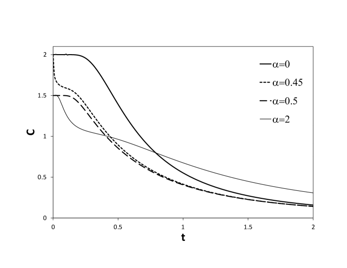
Figure 3: Specific heat as a function of the normalized temperature for the model (2) for several values of $\alpha$.

In Fig. 3 we present the results for the specific heat per triangle as a function of the normalized temperature $t$ for different values of $\alpha$. Note that $\alpha=0.45$ corresponds to the situation in $Fe_{10}Gd_{10}$. As it is seen in Fig. 3 $C(t)$ (in $k_{B}$ units) has different low temperature limits for $\alpha<\frac{1}{2}$ and $\alpha\geq\frac{1}{2}$:

$$C(0) = 2,\qquad\alpha<\frac{1}{2}$$

$$C(0) = \frac{3}{2},\qquad\alpha\geq\frac{1}{2}.$$ (20)

$C(t)$ approaches $2$ in the ferromagnetic region $\alpha<\frac{1}{2}$ because the model is the classical one with two degrees of freedom per spin (four degrees per triangle). But for $\alpha\geq\frac{1}{2}$ the specific heat tends to $\frac{3}{2}$. It means that only three degrees of freedom per triangle contribute to the specific heat and there is one local rotational degree ($\varphi_{3}$) of freedom which costs no energy and gives no contribution to the thermodynamics.

The low temperature behavior of $C(t)$ for $\alpha$ slightly lower the point $\frac{1}{2}$ has the following characteristic feature. $C(t)$ sharply increases from $C\simeq\frac{3}{2}$ to $C=2$ when $t$ tends to zero. As will be shown in Sec. V this feature is consistent with the scaling dependence of physical quantities in the vicinity of the critical point $\alpha=\frac{1}{2}$. According to Eq. (67), see below, the scaling variable is $t/(\alpha-\frac{1}{2})^{2}$. Therefore, we can say that the system behaves as in the critical point $\alpha=\frac{1}{2}$ for temperatures $t>(\alpha-\frac{1}{2})^{2}$, and starts to feel the small deviation from the critical point at very low temperatures $t<(\alpha-\frac{1}{2})^{2}$.

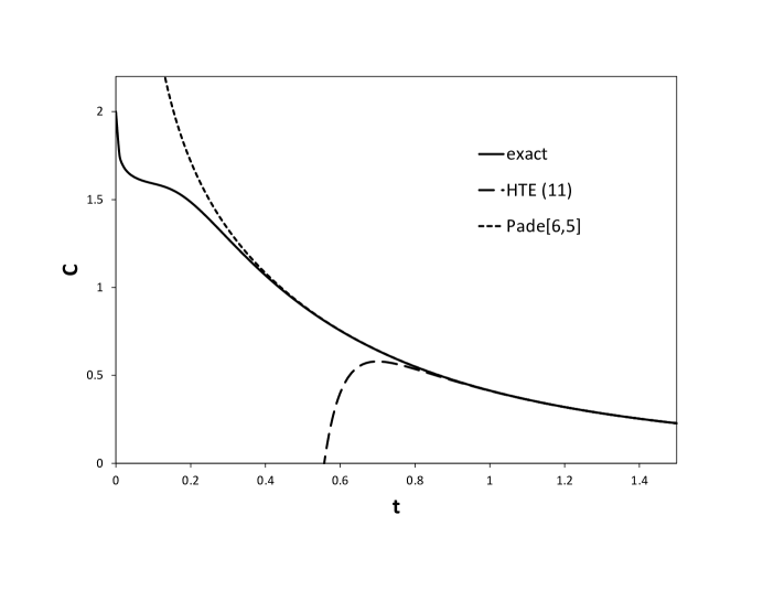
Figure 4: Comparison of the specific heat calculated by 11th-order HTE and the corresponding Pade approximant [6,5] with the exact classical result for $\alpha=0.45$.

For high temperatures we obtained an analytical expansion up to 11-th order in $t^{-1}$ 11order . The leading terms of this high temperature expansion (HTE) are

$$C=\frac{2+\alpha^{2}}{3t^{2}}-\frac{2\alpha}{3t^{3}}+O(t^{-4}).$$ (21)

The results of HTE and the corresponding Pade approximant [6,5] are compared with the exact classical $C(t)$ for $\alpha=0.45$ in Fig. 4. As it is seen in Fig. 4 the raw HTE series coincides with exact result for $t\geq 0.9$ and the Pade approximant [6,5] extends the confidence region up to $t\geq 0.4$.

III.2 Correlation functions

In this subsection we derive the expressions for the spin correlation function $\vec{n}_{i}\cdot\vec{n}_{j}$ and the zero field susceptibility. Since we work with the local coordinate system directed so that the spin vector on each site is directed along the $z$ axis, to find the scalar product of spin vectors $\vec{n}_{l}\cdot\vec{n}_{l+r}$ we need to express the vector $\vec{n}_{l+r}$ in the local coordinate system located on the site $l$. This can be represented as a chain of successive rotations Harada :

$$\vec{n}_{l}\cdot\vec{n}_{l+r}=\left(0,0,1\right)\hat{T}_{2}\hat{T}_{3}\ldots\hat{T}_{r}\left(\begin{array}[]{c}0\\ 0\\ 1\end{array}\right),$$ (22)

where

$$\hat{T}_{i}=\hat{R}^{x}(\theta_{i-1})\hat{R}^{z}(\varphi_{i})$$ (23)

and the rotation operators over the axes $x$ and $z$ are

$$\hat{R}^{x}(\theta) = \left(\begin{array}[]{ccc}1&0&0\\ 0&\cos\theta&\sin\theta\\ 0&-\sin\theta&\cos\theta\end{array}\right)$$ (27)

$$\hat{R}^{z}(\varphi) = \left(\begin{array}[]{ccc}-\cos\varphi&-\sin\varphi&0\\ \sin\varphi&-\cos\varphi&0\\ 0&0&1\end{array}\right).$$ (31)

Then, for the averages one has

$$\left\langle\vec{n}_{l}\cdot\vec{n}_{l+r}\right\rangle=\frac{1}{Z_{\Delta}^{r}}\prod_{i=1}^{r}\frac{1}{4\pi}\int_{0}^{\pi}\sin\theta_{i}d\theta_{i}\int_{0}^{2\pi}d\varphi_{i+1}e^{-\beta H}\cdot\left(0,0,1\right)T_{2}T_{3}\ldots T_{r}\left(\begin{array}[]{c}0\\ 0\\ 1\end{array}\right)\,.$$ (32)

Since total Hamiltonian (5) does not contain the angles $\varphi_{1},\varphi_{3}\ldots$, integration over these angles can be carried out explicitly, which results in

$$\int_{0}^{2\pi}\hat{R}^{z}(\varphi)\frac{d\varphi}{2\pi}=\left(\begin{array}[]{ccc}0&0&0\\ 0&0&0\\ 0&0&1\end{array}\right)=\left(\begin{array}[]{c}0\\ 0\\ 1\end{array}\right)\cdot\left(0,0,1\right).$$ (33)

This implies that the long-distance correlator splits into the product of correlators on all intermediate triangles

$$\left\langle\vec{n}_{1(2)}\cdot\vec{n}_{2r+1(0)}\right\rangle=\left\langle\vec{n}_{1(2)}\cdot\vec{n}_{3}\right\rangle\left\langle\vec{n}_{3}\cdot\vec{n}_{5}\right\rangle\left\langle\vec{n}_{5}\cdot\vec{n}_{7}\right\rangle\ldots\left\langle\vec{n}_{2r-1}\cdot\vec{n}_{2r+1(0)}\right\rangle.$$ (34)

Using the fact that all local correlators of type $\left\langle\vec{n}_{2i-1}\cdot\vec{n}_{2i+1}\right\rangle$ are equal to $\left\langle\vec{n}_{1}\cdot\vec{n}_{3}\right\rangle$ and $\left\langle\vec{n}_{2}\cdot\vec{n}_{3}\right\rangle=\left\langle\vec{n}_{1}\cdot\vec{n}_{2}\right\rangle$ we obtain the expressions for the spin correlation functions:

$$\left\langle\vec{n}_{2n+1}\cdot\vec{n}_{2m+1}\right\rangle = \left\langle\vec{n}_{1}\cdot\vec{n}_{3}\right\rangle^{\left|m-n\right|}$$

$$\left\langle\vec{n}_{2n}\cdot\vec{n}_{2m+1}\right\rangle = \left\langle\vec{n}_{1}\cdot\vec{n}_{2}\right\rangle\left\langle\vec{n}_{1}\cdot\vec{n}_{3}\right\rangle^{\left|m-n\right|}$$

$$\left\langle\vec{n}_{2n}\cdot\vec{n}_{2m}\right\rangle = \left\langle\vec{n}_{1}\cdot\vec{n}_{2}\right\rangle^{2}\left\langle\vec{n}_{1}\cdot\vec{n}_{3}\right\rangle^{\left|m-n\right|-1}.$$ (35)

The local correlators $\left\langle\vec{n}_{1}\cdot\vec{n}_{2}\right\rangle$ and $\left\langle\vec{n}_{1}\cdot\vec{n}_{3}\right\rangle$ are given by Eqs. (17).

As follows from Eq. (35) the spin correlation functions decay exponentially with the correlation length

$$\xi=-\frac{1}{\ln\left|\left\langle\vec{n}_{1}\cdot\vec{n}_{3}\right\rangle\right|}.$$ (36)

The analysis of the behavior of correlation functions (35) will be given in Sec. V.

Now we can calculate the zero-field magnetic susceptibility per spin

$$\chi=\frac{1}{6TN}\sum_{i,j}\left\langle\vec{S}_{i}\cdot\vec{S}_{j}\right\rangle.$$ (37)

Using the obtained correlation functions (35) we arrive at the following expression for the magnetic susceptibility:

$$\chi t=\frac{\left(1+x\left\langle\vec{n}_{1}\cdot\vec{n}_{2}\right\rangle\right)^{2}}{3x(1-\left\langle\vec{n}_{1}\cdot\vec{n}_{3}\right\rangle)}+\frac{x^{2}-1}{6x},$$ (38)

where $x=S_{a}/S_{b}$.

The high temperature behavior of the susceptibility is obtained in the analytical form up to 11-th order in $t^{-1}$ 11order . The leading terms of HTE at $x=1$ are

$$\chi(t)=\frac{1}{3t}+\frac{2-\alpha}{9t^{2}}+\frac{2-4\alpha+\alpha^{2}}{27t^{3}}+O(t^{-4})$$ (39)

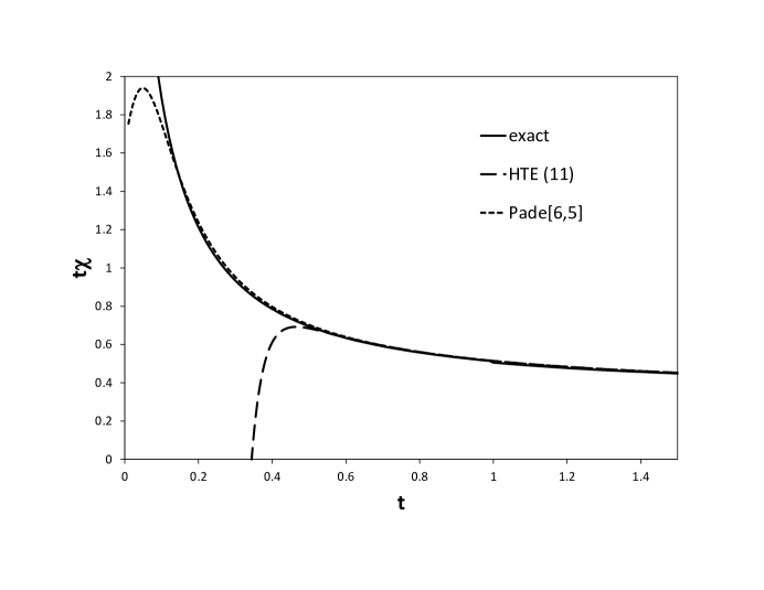
Figure 5: Comparison of the susceptibility calculated by 11th-order HTE and the corresponding Pade approximant [6,5] with the exact classical result for $\alpha=0.45$.

The dependencies $\chi(t)$ obtained by HTE up to 11-th order and the corresponding Pade approximant [6,5] for $\alpha=0.45$ are compared with the exact result in Fig. 5. As one can see in Fig. 5 the raw HTE series separates from the exact result at $t\sim 0.5$, whereas the Pade approximant [6,5] coincides with the exact result up to $t\sim 0.2$.

In the case of the ferromagnetic short-range order, when spins on one triangle $\vec{n}_{1},\vec{n}_{2},\vec{n}_{3}$ are almost parallel, the correlation length (36) is large and the susceptibility relates to the correlation length as

$$\chi t=\frac{\left(1+x\right)^{2}}{3x}\xi.$$ (40)

IV Low temperature limit

In general, Eq. (38) completely describes the behavior of the magnetic susceptibility as a function of the temperature and the frustration parameter $\alpha$. However, in this Section we pay special attention to the low temperature limit, where the explicit analytical results will help us to establish the scaling law near the critical point.

At $T\to 0$ the integration in Eq. (11) can be carried out using the saddle point method. For this aim we need to expand the exponent in Eq. (11) near the ground state of the triangle Hamiltonian (9). Since the ground state of $H_{\Delta}$ is different in the regions $\alpha<\frac{1}{2}$ and $\alpha>\frac{1}{2}$ and at the transition point $\alpha=\frac{1}{2}$, it is necessary to study these three cases separately.

IV.1 The case $\alpha<\frac{1}{2}$

In the case $\alpha<\frac{1}{2}$ all spins pointing in the same direction ($\theta_{i}=0$) in the ground state of $H_{\Delta}$ and we expand the exponent in Eq. (11) near the energy minimum, so that the partition function (11) takes the form

$$Z_{\Delta}=\frac{1}{8\pi}e^{(2-\alpha)\beta}\int_{0}^{\infty}\theta_{1}d\theta_{1}\int_{0}^{\infty}\theta_{2}d\theta_{2}\int_{0}^{2\pi}d\varphi_{2}\exp\left[-\frac{1}{2}\beta(1-\alpha)(\theta_{1}^{2}+\theta_{2}^{2})-\beta\alpha\theta_{1}\theta_{2}\cos\varphi_{2}\right].$$ (41)

Performing the integration we obtain

$$Z_{\Delta}=\frac{\exp\left(2\beta-\alpha\beta\right)}{4\beta^{2}\left(1-2\alpha\right)}.$$ (42)

The correlator $\left\langle\vec{n}_{1}\cdot\vec{n}_{2}\right\rangle=\left\langle\cos\theta_{1}\right\rangle$ in the low-temperature limit is

$$\left\langle\vec{n}_{1}\cdot\vec{n}_{2}\right\rangle=1-\frac{1}{2}\left\langle\theta_{1}^{2}\right\rangle.$$ (43)

We omit technical details and give the expression for the expectation value $\left\langle\theta_{1}^{2}\right\rangle$:

$$\left\langle\theta_{1}^{2}\right\rangle=2t\frac{1-\alpha}{1-2\alpha}.$$ (44)

The correlator $\left\langle\vec{n}_{1}\cdot\vec{n}_{3}\right\rangle$ given by Eq. (17) is calculated in a similar way, which yields:

$$\left\langle\vec{n}_{1}\cdot\vec{n}_{2}\right\rangle = 1-t\frac{1-\alpha}{1-2\alpha}$$

$$\left\langle\vec{n}_{1}\cdot\vec{n}_{3}\right\rangle = 1-t\frac{2}{1-2\alpha}.$$ (45)

Now, substituting Eqs. (45) into Eq. (38) we obtain the low-temperature limit for the susceptibility in the case $\alpha<\frac{1}{2}$

$$\chi t=\frac{(1-2\alpha)\left(1+x\right)^{2}}{6tx}.$$ (46)

IV.2 The case $\alpha=\frac{1}{2}$

In the case $\alpha=\frac{1}{2}$ the ground state of $H_{\Delta}$ is ferromagnetic as well as for the case $\alpha<$ $\frac{1}{2}$. However, the denominator ($1-2\alpha$) presented in Eqs. (42), (44), (45) indicates that the case $\alpha=\frac{1}{2}$ is special and it is necessary to keep more terms in the expansion of the energy near the minimum:

$$H_{\Delta}=-\frac{3}{2}+\frac{1}{4}(\theta_{1}-\theta_{2})^{2}-\frac{1}{48}(\theta_{1}-\theta_{2})^{4}+\frac{1}{4}\theta_{1}^{2}\theta_{2}^{2}+\frac{1}{2}\theta_{1}\theta_{2}(1+\cos\varphi_{2}).$$ (47)

The form of Hamiltonian (47) suggests to change variables as

$$\theta_{1} = ut^{1/4}+vt^{1/2}$$

$$\theta_{2} = ut^{1/4}-vt^{1/2}.$$ (48)

Then to the lowest power in $t$ Hamiltonian (47) becomes:

$$\beta H_{\Delta}=-\frac{3\beta}{2}+v^{2}+\frac{1}{4}u^{4}+\sqrt{\beta}\frac{1+\cos\varphi_{2}}{2}u^{2}.$$ (49)

Substituting Eq. (49) into the partition function (11) and integrating it over $\varphi_{2}$ we get

$$Z_{\Delta}=\frac{1}{2}e^{\frac{3}{2}\beta}\beta^{-5/4}\int_{0}^{\infty}u^{2}du\int_{0}^{\infty}dv\exp\left(-v^{2}-\frac{1}{4}u^{4}-\frac{1}{2}\sqrt{\beta}u^{2}\right)I_{0}\left(\frac{1}{2}\sqrt{\beta}u^{2}\right).$$ (50)

Now we notice that the argument of the Bessel function in Eq. (50) tends to infinity at $t\to 0$ and we can use the asymptotic form of the Bessel function

$$I_{0}\left(x\to\infty\right)=\frac{e^{x}}{\sqrt{2\pi x}}.$$ (51)

Then the partition function can be integrated which yields

$$Z_{\Delta}=\frac{\sqrt{\pi}}{8}\beta^{-3/2}\exp\left(\frac{3}{2}\beta\right).$$ (52)

The mean value of $\theta_{1}^{2}$ in this case is

$$\left\langle\theta_{1}^{2}\right\rangle=\beta^{-1/2}\left\langle u^{2}\right\rangle=\frac{2}{\sqrt{\pi\beta}}$$ (53)

which results in the following expressions for the correlators:

$$\left\langle\vec{n}_{1}\cdot\vec{n}_{2}\right\rangle = 1-\frac{1}{\sqrt{\pi\beta}}$$

$$\left\langle\vec{n}_{1}\cdot\vec{n}_{3}\right\rangle = 1-\frac{4}{\sqrt{\pi\beta}}.$$ (54)

Then, the leading term for susceptibility (38) in the low-temperature limit in the critical point $\alpha=\frac{1}{2}$ is

$$\chi t=\frac{\sqrt{\pi}\left(1+x\right)^{2}}{12xt^{1/2}}.$$ (55)

IV.3 The case $\alpha>\frac{1}{2}$

As was discussed in Sec. II the ground state of one triangle in the region $\alpha>\frac{1}{2}$ is a ferrimagnetic one. Therefore, in this case we expand the Hamiltonian (9) around the ferrimagnetic classical spin configuration:

$$H_{\Delta}=-\frac{1}{2\alpha}-\alpha+(\alpha-\frac{1}{2\alpha})xy+\frac{\alpha}{2}(x^{2}+y^{2})+(2\alpha-\frac{1}{2\alpha})z^{2},$$ (56)

where variables $x,y,z$ describe the deviations around the ground state

$$\theta_{1} = \theta_{0}+x$$

$$\theta_{2} = \theta_{0}+y$$

$$\varphi_{2} = \pi+2z.$$ (57)

The partition function in this case can be written in the form

$$Z_{\Delta}=\frac{\sin^{2}\theta_{0}}{8\pi}\int_{-\infty}^{\infty}e^{-\beta H_{\Delta}}dxdydz$$ (58)

and after integration one obtains

$$Z_{\Delta}=\beta^{-3/2}\sqrt{\frac{\pi}{32\alpha}}\exp\left(\frac{\beta}{2\alpha}+\beta\alpha\right).$$ (59)

Spin correlators $\left\langle\vec{n}_{1}\cdot\vec{n}_{2}\right\rangle$ and $\left\langle\vec{n}_{1}\cdot\vec{n}_{3}\right\rangle$ are given by the ground state configuration (7), thermal fluctuations in the region $\alpha>\frac{1}{2}$ are irrelevant for the calculation of the leading term in the susceptibility:

$$\chi t=\frac{\left(2\alpha x+1\right)^{2}}{6x(4\alpha^{2}-1)}.$$ (60)

Summarizing our findings for the susceptibility $\chi(t)$ we may conclude that the power-law divergence as $t\to 0$ is different in all three regimes $\alpha<\frac{1}{2}$, $\alpha=\frac{1}{2}$, $\alpha>\frac{1}{2}$, see Eqs. (46), (55), and (60).

V Scaling near the critical point and finite size effect

In this section we analyze the obtained analytical results for low temperatures and estimate the finite-size effect. As follows from Eqs. (45) and (54) the correlation length (36) has different low-temperature behavior in different regions:

$$\xi = \frac{1-2\alpha}{2t},\qquad\alpha<\frac{1}{2}$$ (61)

$$\xi = \frac{1}{4}\sqrt{\frac{\pi}{t}},\qquad\alpha=\frac{1}{2}$$ (62)

$$\xi = \left[\ln\left|\frac{2\alpha^{2}}{1-2\alpha^{2}}\right|\right]^{-1},\qquad\alpha>\frac{1}{2}\;.$$ (63)

For $\alpha<\frac{1}{2}$ the correlation length diverges in the low-temperature limit as $\xi\sim 1/t$ similar to the classical ferromagnetic chain ($\alpha=0$). In the critical point $\alpha=\frac{1}{2}$ the correlation length diverges as well, but by another law $\xi\sim t^{-1/2}$. In the region $\alpha>\frac{1}{2}$ the correlation length remains finite at $t=0$. This fact is directly related to the macroscopic degeneracy of the ground state discussed in Sec. II, which causes the rapid decay of the correlation between spins even at zero temperature.

As follows from Eq. (63), there are two special cases $\alpha=1/2$ and $\alpha=1/\sqrt{2}$ where the correlation length is zero. The case $\alpha=1/2$ correspond to the critical point, and we will analyze the behavior of the system near the critical point later.

The case $\alpha=1/\sqrt{2}$ is special, because according to Eq. (7) the angle $\theta_{0}=\pi/4$, so that adjacent basal spins in the ground state are orthogonal, $\vec{n}_{1}\cdot\vec{n}_{3}=0$. This leads to the fact that all correlators in Eqs. (35) become zero. However, this does not mean that all spins at this point become independent. Instead this is the point where the ferromagnetic type of correlations of basal spins $\left\langle\vec{n}_{1}\cdot\vec{n}_{2m+1}\right\rangle\sim\exp(-m/\xi)$ turns into the AF type: $\left\langle\vec{n}_{1}\cdot\vec{n}_{2m+1}\right\rangle\sim(-1)^{m}\exp(-m/\xi)$ for $\alpha>1/\sqrt{2}$. So, this is not a transition point and thermodynamic quantities have no singularity at $\alpha=1/\sqrt{2}$.

Now let us analyze the correlation function in the ferrimagnetic region $\alpha>\frac{1}{2}$ at $T=0$. In absence of thermal fluctuations the system is in the ground state and the angle between nearest basal spins is fixed and equal to $2\theta_{0}$ according to Eq. (7). However, as was noted in Sec. II the spins in each triangle can lie in any plane, which leads to the degeneracy of the ground state. Each ground state spin configuration can be represented as a sequence of points lying on the unit sphere with an equal distance between neighboring points in the sequence as shown in Fig. 2. Thus, the problem of the spin correlations at zero temperature is equivalent to the problem of a random walk with fixed finite step length $2\theta_{0}$ on a unit sphere. Eq. (35) gives the exact solution of this problem

$$\cos(2\theta_{m})=\cos^{m}(2\theta_{0})\;,$$ (64)

where the angle $\theta_{m}$ is defined by the relation: $\cos(2\theta_{m})=\left\langle\vec{n}_{1}\cdot\vec{n}_{2m+1}\right\rangle$. Eq. (64) is valid for any value of the step length. In particular, when the step of the random walk is small $2\theta_{0}\ll 1$ ($\alpha$ is close to the critical point) and the number of steps is not very large, $\theta_{m}\lesssim 1$, one can expand both sides of Eq. (64) and reproduce the common diffusion law:

$$\theta_{m}=\sqrt{m}\theta_{0}\;.$$ (65)

Returning to the language of the correlation function, we note that the condition of the validity of Eq. (65), $\theta_{m}\lesssim 1$, provides an estimate of the correlation length $\xi=m$ as $\xi\sim\theta_{0}^{-2}$, which is in accord with Eq. (63) for $\alpha$ close to $\frac{1}{2}$.

The analysis of Eqs. (61), (62), (63) in the vicinity of the point $\alpha=\frac{1}{2}$ allows us to write the correlation length in the scaling form:

$$\xi(\alpha,t)=\frac{1}{4\sqrt{t}}f\left(y\right)\;,$$ (66)

where the scaling parameter

$$y=\frac{2\alpha-1}{\sqrt{t}}\;,$$ (67)

and the scaling function $f(y)$ has the following asymptotic:

$$f(y) \sim -2y,\qquad y\to-\infty$$

$$f(y) \sim 1/y,\qquad y\to\infty$$ (68)

and $f(0)=\sqrt{\pi}$. The scaling function calculated for different $\alpha$ and $T$ is shown in Fig. 6.

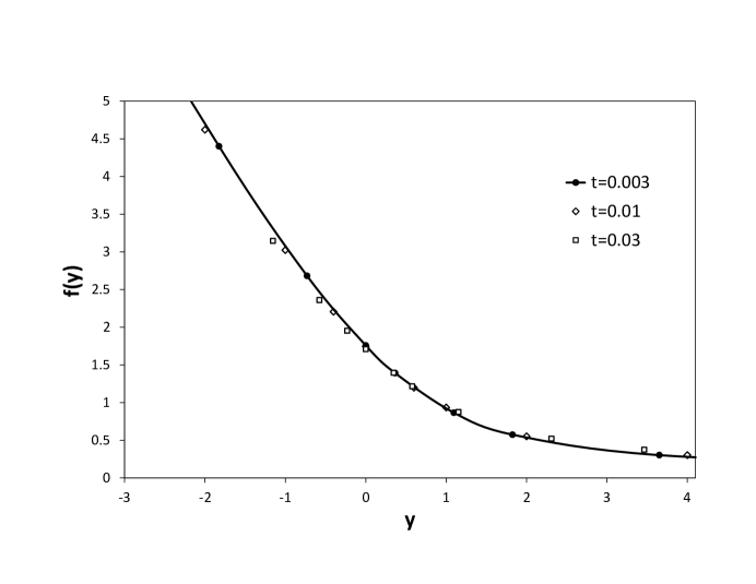
Figure 6: Scaling function $f(y)$ for the correlation length and the susceptibility in the vicinity of the critical point $\alpha=\frac{1}{2}$ calculated for different values of $\alpha$ and $t$. All data lie on one curve, which confirms the scaling law.

Next we note that in the vicinity of the critical point the correlation length is large, which allows us to use the relation between the susceptibility and the correlation length (40):

$$t\chi(\alpha,t)=\frac{\left(1+x\right)^{2}}{12x\sqrt{t}}f(y)\;.$$ (69)

Eq. (69) describes the scaling form of the susceptibility in the vicinity of the critical point and correctly reproduces Eqs. (46), (55), (60) in the corresponding limits.

In order to estimate the finite size effect one needs to compare the chain length with the correlation length, so that another scaling parameter $N/\xi$ appears. All above results correspond to the thermodynamic limit when $N\gg\xi$. However, for a finite chain and low enough temperatures, when $N<\xi$, another regime takes place. For example, the susceptibility per site in the short chain case $N<\xi$ as follows from Eq. (37) is

$$t\chi=\frac{(1+x)^{2}}{6x}N\;.$$ (70)

This behavior is obviously a non-thermodynamic one. Here we notice that Eq. (69) reduces to Eq. (40) with substitution $\xi=N/2$. This allows us to write the scaling form for the susceptibility in the vicinity of the point $\alpha=\frac{1}{2}$

$$t\chi(\alpha,t,N)=\frac{\left(1+x\right)^{2}}{3x}\xi(\alpha,t)F\left(\frac{2\xi(\alpha,t)}{N}\right)$$ (71)

with $\xi(\alpha,t)$ given by Eq. (66). The scaling function $F(z)$ describes the finite-size effect and has the limits $F(0)=1$ and $F(y)=1/z$ at $z\to\infty$, smoothly switching between Eqs. (40) and (70). As follows from Eq. (71) the finite-size effects become important for low temperatures and $\alpha\leq\frac{1}{2}$, when the correlation length is large. In the region $\alpha>\frac{1}{2}$ the correlation length $\xi$ is finite even at zero temperature and, therefore, the thermodynamics converges rapidly with $N$.

VI Quantum effects

In this section we ascertain a relation of the thermodynamic properties of the classical model (2) with those of the quantum delta chain (1). We are mainly interested in the role of quantum effects in the ferromagnetic phase ($\alpha<\frac{1}{2}$) and especially for the frustration parameter of the $Fe_{10}Gd_{10}$ system, i.e. $\alpha=0.464$ ($a=0.65$). The classical approximation corresponds to the spin quantum numbers $S\to\infty$. It is known that even for a system with relatively large values of spins quantum effects become essential at low temperatures. The analysis of thermodynamic properties of the quantum model is performed by a combination of high temperature series expansion (HTE) 11order , exact diagonalization (ED) spinpack and finite-temperature Lanczos (FTL) technique FTL1 ; FTL2 (where ED and FTL work only for finite delta chains) as well as by the modified spin-wave theory (MSWT) MSWT . For simplicity we consider next, if not mentioned otherwise, the delta chain model with $S_{a}=S_{b}=S$.

We start our analysis with the estimate of the quantum corrections to the classical results for high temperatures. For this aim we use HTE for the quantum delta chain in powers of $T^{-1}$. Such expansion has been calculated up to 11th order using the code of Ref. 11order . The first three terms of HTE for the specific heat are

$$C(S,T) = \frac{X^{2}(2+\alpha^{2})}{3T^{2}}-\frac{4X^{3}\alpha-X^{2}(2+\alpha^{3})}{6T^{3}}$$ (72)

$$-\frac{(3X^{4}+8X^{3}-3X^{2})(2+\alpha^{4})+5X^{3}(2\alpha+5\alpha^{2})}{45T^{4}}+O(T^{-5})\;,$$

where $X=S(S+1)$. The HTE for the susceptibility has a similar structure:

$$\chi(S,T)=\frac{X}{3T}+\frac{X^{2}(2-\alpha)}{9T^{2}}+\frac{X^{3}(2-4\alpha+\alpha^{2})-\frac{3}{4}X^{2}(2+\alpha^{2})}{27T^{3}}\;.$$ (73)

As follows from Eqs. (72) and (73) each HTE term proportional to $\sim T^{-m}$ contains a factor which is a polynomial of the order $m$ in $S(S+1)$. The leading terms of these polynomials are described by the classical approximation (21). Moreover, it turns out that the first term of the HTE series (72) is exactly reproduced by the classical expansion (21) after the substitution $t=T/S(S+1)$. Therefore, the leading term of the difference between the classical and the quantum expansions is of the order of $T^{-3}$:

$$C(S,T)-C_{class}(T)=\frac{X^{2}(2+\alpha^{3})}{6T^{3}}+O(T^{-4})$$ (74)

and, similar,

$$\chi(S,T)-\chi_{class}(T)=-\frac{X^{2}(2+\alpha^{2})}{36T^{3}}+O(T^{-4})\;.$$ (75)

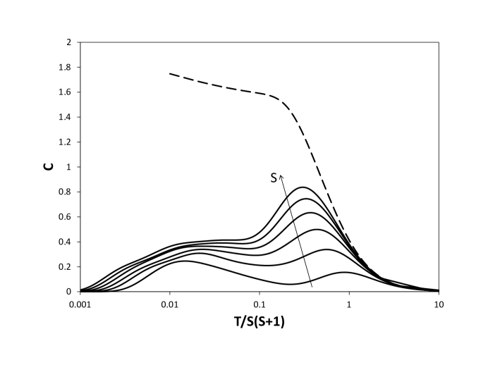
Figure 7: Specific heat as a function of the normalized temperature for the quantum spin model (1) for $\alpha=0.45$ calculated by ED and FTL for finite $N=6$ chain. The curves with spin $S=\frac{1}{2},1,\frac{3}{2},2,\frac{5}{2},3$ are arranged in order from bottom to top. Specific heat for classical model is shown by dashed line.

The temperature range where HTE gives reliable results is of the order of $T/S(S+1)\sim 1$, see also Ref. 11order . For the analysis of the thermodynamic properties of the quantum model at low temperatures $T/S(S+1)<1$ we carried out numerical ED and FTL calculations for finite delta chains. In Fig. 7 we present the temperature dependence of the specific heat for a delta chain of $N=6$ unit cells for different spin values from $S=\frac{1}{2}$ to $S=3$, where we consider the frustration parameter $\alpha=0.45$ which is close to the critical point $\alpha_{c}=\frac{1}{2}$ and is related to the situation in $Fe_{10}Gd_{10}$. As shown in Fig. 7 all curves with different spin coincide with the classical $C(T)$ for $T\geq S(S+1)$ and deviate from the classical curve and from each other at $T\sim S(S+1)$, in accord with the prediction of HTE (74). It is also seen in Fig. 7 that for $S=\frac{1}{2},1,\frac{3}{2}$ the specific heat exhibits a two-peak structure with maxima at low and intermediate temperatures. With increasing $S$ the height of the second maximum increases and its position along the $T/S(S+1)$-axis shifts to the left. The low-temperature maximum transforms to a shoulder for $S\geq 2$. In particular, such shoulder exists (as shown in Fig. 8) in the delta-chain with $N=6$ and $S_{a}=\frac{7}{2},$ $S_{b}=\frac{5}{2}$ ($a=0.65$) modeling the fictitious ‘magnetic molecule’ $Fe_{6}Gd_{6}$.

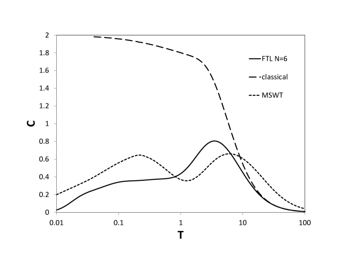
Figure 8: Specific heat as a function of temperature for the $Fe_{10}Gd_{10}$ parameter set ($a=0.65$, $S_{a}=\frac{7}{2}$, $S_{b}=\frac{5}{2}$) calculated by the FTL method for $N=6$ (solid line), in classical approximation (dashed line) and in MSWT approach (dotted line).

Unfortunately, the ED and FTL calculations have the following limitation: the higher the spin value the shorter the chain that can be calculated, so that for $S>3$ calculations even for $N=6$ are impossible because the Hilbert space dimension becomes too large. Besides, because of the finite-size energy gaps in the spectrum the finite chain calculations cannot correctly describe the low temperature behavior of the system in the thermodynamic limit $N\to\infty$. Therefore, a complementary approach is needed to overcome these shortcomings of finite-chain calculations. We use an approximate method based on the modified spin wave theory MSWT . In this method the spin operators are replaced by bosonic operators as in the standard spin-wave theory and the constraint of zero total magnetization at finite temperature is imposed. This approach has been successfully applied to low-dimensional Heisenberg models MSWT ; Yamamoto ; Sirker . Retaining only the lowest order in the spin-bosonic transformation terms we obtain a bilinear bosonic Hamiltonian, which after the diagonalization takes a form

$$\hat{H}=\sum\varepsilon_{A}(k)A_{k}^{\dagger}A_{k}+\varepsilon_{B}(k)B_{k}^{\dagger}B_{k}\;,$$ (76)

where two magnon branches $\varepsilon_{A,B}(k)$ are

$$\varepsilon_{A,B}(k)=2S(1-\alpha\sin^{2}\frac{k}{2})\pm 2S\sqrt{(1-\alpha\sin^{2}\frac{k}{2})^{2}-(1-2\alpha)\sin^{2}\frac{k}{2}}\;.$$ (77)

The energy is

$$E=\sum[\varepsilon_{A}(k)n_{A}(k)+\varepsilon_{B}(k)n_{B}(k)]\;.$$ (78)

Here the mean values of the occupations $n_{A}(k)=\left\langle A_{k}^{\dagger}A_{k}\right\rangle$ and $n_{B}(k)=\left\langle B_{k}^{\dagger}B_{k}\right\rangle$ are given by the Bose-Einstein distribution:

$$n_{A,B}(k)=\left[\exp\left(\frac{\varepsilon_{A,B}(k)-\mu}{T}\right)-1\right]^{-1}$$ (79)

and the chemical potential $\mu$ is defined by the condition of zero total magnetization:

$$\frac{1}{N}\sum[n_{A}(k)+n_{B}(k)]=2S\;.$$ (80)

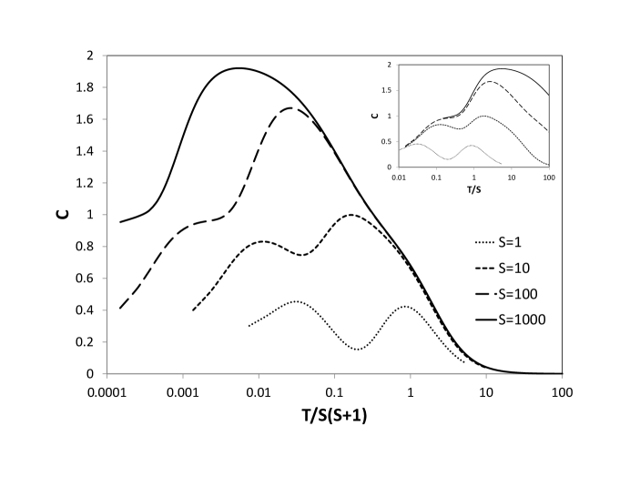
Figure 9: Specific heat as a function of the normalized temperature for the quantum spin model (1) for $\alpha=0.45$ in MSWT approach for $S=1,10,100,1000$. In the inset the same curves are plotted vs. $T/S$.

The results of the MSWT calculations of the specific heat for $\alpha=0.45$ are presented in Fig. 9. As can be seen from Fig. 9 the specific heat for $S=1$ exhibits a double-peak structure similar to that in Fig. 7. Such a structure is related to the fact that the lower $\varepsilon_{A}$ and the higher $\varepsilon_{B}$ magnon branches give distinct contributions to $C(T)$ at low and intermediate temperatures because these branches are well separated for $\alpha$ close to $\frac{1}{2}$. In this case the gap between the branches is $\Delta E=4S\alpha$. At low temperatures $C(T)$ is determined by the lower branch which behaves at $k\to 0$ as

$$\varepsilon_{A}(k)=\frac{S(1-2\alpha)}{4}k^{2}\;.$$ (81)

The lower branch sets the low-energy scale leading to a low-temperature peak in the specific heat. The low-temperature maximum exists even for $S=10$ contrary to the results of the ED and the FTL calculations and this maximum transforms to the shoulder for $S\sim 100$ only. This means that the MSWT approximation overestimates the value of $C(T)$ at low temperature. The second maximum increases with growing $S$ and tends to the classical value $C=2$ as $S\to\infty$. Its position shifts to the left of the $T/S(S+1)$-axis with increasing $S$, which is in agreement with ED and FTL results. Such behavior is a consequence of the fact that in the MSWT approximation the temperature $T$ and the spin value $S$ form a scaling variable $T/S$ at low temperatures (because $\varepsilon_{A,B}\sim S$ and $\mu\sim T^{2}/S^{3}$ give negligible contributions at low $T$). Therefore, the low temperature behavior of the delta chain with high value of $S$ is a function of $T/S$ and, therefore, the shoulder and the maximum in the specific heat are located at $T\sim S$ as illustrated in the inset of Fig. 9.

The specific heat of the quantum model tends to zero in the limit $T\to 0$. It is believed that the spin-wave approach gives the true leading term in this limit:

$$C(T)=\frac{3\zeta(\frac{3}{2})}{4\sqrt{\pi}}\sqrt{\frac{T}{(1-2\alpha)S}}\;.$$ (82)

This result is related to the infinite delta-chain. For finite systems such as $Fe_{10}Gd_{10}$ the specific heat vanishes exponentially in $1/T$ at $T\to 0$. In contrast to the quantum case, the classical specific heat is finite at $T=0$. Therefore, the behavior of the specific heat at low temperatures of the classical and the quantum delta chain is essentially different.

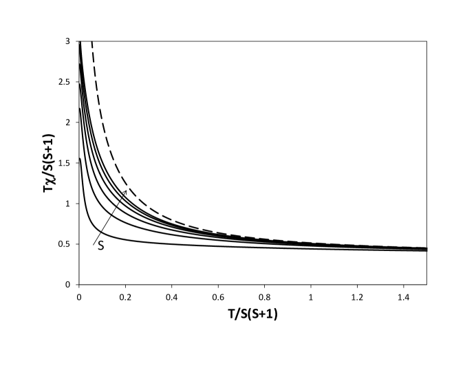
Figure 10: Susceptibility as a function of the normalized temperature for the quantum spin model (1) for $\alpha=0.45$ calculated by ED and FTL for finite $N=6$ chain. The curves with spin $S=\frac{1}{2},1,\frac{3}{2},2,\frac{5}{2},3$ are arranged in order from bottom to top. The susceptibility for the classical model is shown by dashed line.

However, in some cases the low-temperature properties of the quantum and the classical models are very similar. For example, both classical and quantum ferromagnetic chains have the same universal magnetic low-temperature behavior Nakamura ; Sachdev ; Bacalis . Similarly, such universality holds for the F-AF chain as well DK11 . In analogy to these models we can expect that the low-temperature behavior of the zero-field susceptibility $\chi(T)$ of the classical and the quantum delta-chain in the ferromagnetic phase are also the same. The dependencies of the product $\chi T$ of the classical delta chain and the quantum model with $N=6$ and different $S$ are shown in Fig. 10 for $\alpha=0.45$. With increasing $S$ the quantum curves approach the classical one. The low-temperature susceptibility in the MSWT approximation is

$$\chi=\frac{4(1-2\alpha)S^{4}}{3T^{2}}-\frac{2\zeta(\frac{1}{2})(1-2\alpha)^{1/2}S^{5/2}}{\pi^{1/2}T^{3/2}}+\ldots\;\;.$$ (83)

The comparison of Eqs. (83) and (46) shows that the leading terms of the classical and the quantum susceptibility at $T\to 0$ coincide. We note also that the leading low-temperature term for the correlation length in quantum model coincides with the classical result (61), $\xi=(\frac{1}{2}-\alpha)S^{2}/T$. According to Eq.(83) the susceptibility $\chi(T)$ for infinite system diverges as $T^{-2}$. However, for finite systems and very low temperatures, when $(\frac{1}{2}-\alpha)S^{2}>NT$, $\chi(T)$ diverges as $T^{-1}$. It is due to the fact that according to Eq. (61) the correlation length at $T\to 0$ exceeds the system size and the product $\chi T$ at $T=0$ is

$$\chi T = \frac{4}{3}N^{2}S^{2}$$

$$\chi T = \frac{4}{3}N^{2}S^{2}(1+\frac{1}{2NS})$$ (84)

for the classical and the quantum model, respectively. The term in parenthesis in Eq. (84) is the quantum correction to the classical result.

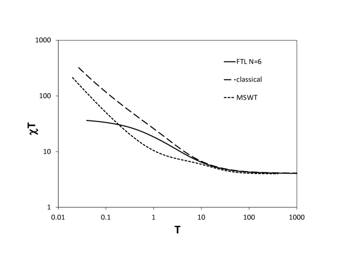
Figure 11: Susceptibility as a function of temperature for the $Fe_{10}Gd_{10}$ parameter set ($a=0.65$, $S_{a}=\frac{7}{2}$, $S_{b}=\frac{5}{2}$) calculated by the FTL method for $N=6$ (solid line), in classical approximation (dashed line) and in MSWT approach (dotted line).

According to Eq. (84) $\chi T$ tends to finite value at $T=0$ for finite systems including real compound containing molecules $Fe_{10}Gd_{10}$ and such behavior is visualized in Fig. 10 and Fig. 11.

VII Summary

In this paper we have studied the delta-chain with competing ferro- and antiferromagnetic interactions. This model finds its finite-size material realization in the recently synthesized cyclic compound $Fe_{10}Gd_{10}$ S60 . In dependence on the frustration parameter $\alpha$ it exhibits ferromagnetic and ferrimagnetic ground-state phases separated by a critical point at $\alpha=1/2$, where the ground state of the quantum model at this point exhibits a massive degeneracy. For the classical version of this model, which seems to provide a reasonable description $Fe_{10}Gd_{10}$ down to moderate temperatures, we obtain exact results for the partition function and the thermodynamics. The explicit analytical expansion of thermodynamic quantities is provided for high temperatures. The low temperature behavior of the specific heat and the susceptibility of the classical model is different in various phases. In the ferromagnetic phase ($\alpha<\frac{1}{2}$) $C(T)=2$ at $T=0$, while $C(0)=\frac{3}{2}$ in the ferrimagnetic phase ($\alpha>\frac{1}{2}$). The zero-field susceptibility diverges as $T^{-2}$ and $T^{-1}$ for $\alpha<\frac{1}{2}$ and $\alpha>\frac{1}{2}$, respectively. In the critical point $\alpha=\frac{1}{2}$ the susceptibility behaves as $\chi\sim T^{-3/2}$.

The classical model corresponds to the limit $S\to\infty$. Quantum corrections to the classical results for large but finite $S$ are small at high temperature ($T>S^{2}$). However, the quantum effects become essential at low temperature. In particular, the classical specific heat is finite at $T=0$, while $C(T)\sim\sqrt{T/S(1-2\alpha)}$ in the infinite quantum model for $\alpha<\frac{1}{2}$ and it is exponentially small at $T\to 0$ for finite delta-chain such as $Fe_{10}Gd_{10}$ magnetic molecule. On the other hand, the leading term of the susceptibility of the classical and the quantum models coincide for both small and large temperatures at $\alpha<\frac{1}{2}$. The product $\chi T$ diverges as $T^{-1}$ at $T\to 0$ for $\alpha<\frac{1}{2}$ in the infinite chain and it is proportional to $N^{2}$ for finite systems. Such behavior of $\chi T$ takes place, in particular, in the $Fe_{10}Gd_{10}$ molecule.

The $C(T)$ dependence in the ferromagnetic phase is characterized by the existence of a two-peak structure for $S<2$. For $S\geq 2$ the low-temperature maximum transforms to the shoulder. Such a $C(T)$ profile with a shoulder and a maximum was observed for the magnetic part of $C(T)$ of $Fe_{10}Gd_{10}$ S60 . The shoulder and the maximum shift towards higher temperature as $S$ increases and $T_{\max}\sim S$.

References

- (1) H. T. Diep (ed) 2013 Frustrated Spin Systems (Singapore: World Scientific).
- (2) C. Lacroix, P. Mendels and F. Mila, eds., Intoduction to frustrated magnetism. Materials, Experiments, Theory (Springer-Verlag, Berlin, 2011).
- (3) Quantum Magnetism, Lecture Notes in Physics 645, edited by U. Schollwöck, J. Richter, D. J. J. Farnell, and R. F. Bishop (Springer-Verlag, Berlin, Heidelberg, 2004).
- (4) O. Derzhko, J. Richter, M. Maksymenko, Int. J. Modern Phys. 29, 1530007 (2015).
- (5) M. E. Zhitomirsky and H. Tsunetsugu, Phys. Rev. B 70, 100403 (2004).
- (6) J. Schnack, H.-J. Schmidt, J. Richter and J. Schulenberg, Eur. Phys. J. B 24, 475 (2001).
- (7) J. Richter, J. Schulenburg, A. Honecker, J. Schnack, and H.J. Schmidt, J. Phys.: Condens. Matter 16, S779 (2004).
- (8) O. Derzhko and J. Richter, Phys. Rev. B 70, 104415 (2004).
- (9) T. Tonegawa and M. Kaburagi, J. Magn. Magn. Materials, 272, 898 (2004).
- (10) V. Ya. Krivnov, D. V. Dmitriev, S. Nishimoto, S.-L. Drechsler, and J. Richter, Phys. Rev. B 90, 014441 (2014).
- (11) D. Leykam, A. Andreanov, S. Flach, Adv. Phys.: X 3, 1473052 (2018).
- (12) Y. Inagaki, Y. Narumi, K. Kindo, H. Kikuchi, T. Kamikawa, T. Kunimoto, S. Okubo, H. Ohta, T. Saito, H. Ohta, T. Saito, M. Azuma, H. Nojiri, M. Kaburagi and T. Tonegawa, J. Phys. Soc. Jpn. 74, 2831 (2005).
- (13) M. Kaburagi, T. Tonegawa and M. Kang, J.Appl.Phys. 97, 10B306 (2005).
- (14) C. Ruiz-Perez, M. Hernandez-Molina, P. Lorenzo-Luis, F. Lloret, J. Cano, and M. Julve, Inorg. Chem. 39 3845 (2000).
- (15) A. Baniodeh, N. Magnani, Y. Lan, G. Buth, C. E. Anson, J. Richter, M. Affronte, J. Schnack, A. K. Powell, npj Quantum Materials 3, 10 (2018).
-
(16)
J. Richter, J. Schulenburg, Eur. Phys. J. B 73, (2010)
117 (2010);
https://www-e.uni-magdeburg.de/jschulen/sp - (17) J. Jaklič and P. Prelovsek, Phys. Rev. B 49, 5065 (1994); Adv. Phys. 49, 1 (2000).
- (18) J. Schnack and O. Wendland, Eur. Phys. J. B B 78, 535 (2010); J. Schnack, J. Schulenburg and J. Richter, Phys. Rev. B 98, 094423 (2018).
- (19) I. Harada and H. J. Mikeska, Z. Phys. B: Condens. Matter 72, 391 (1988).
- (20) A. Lohmann, Diploma Thesis, University Magdeburg 2012; H.-J. Schmidt, A. Lohmann, and J. Richter, Phys. Rev. B 84, 104443 (2011); A. Lohmann, H.-J. Schmidt, and J. Richter, Phys. Rev. B 89, 014415 (2014).
- (21) H. Nakamura and M. Takahashi, J. Phys. Soc. Jpn. 63, 2563 (1994).
- (22) M. Takahashi, H. Nakamura, and S. Sachdev, Phys. Rev. B 54, R744 (1996).
- (23) N. Theodorakopoulos and N. C. Bacalis, Phys. Rev. B 55, 52 (1997).
- (24) D. V. Dmitriev and V. Ya. Krivnov, Phys. Rev. B 82, 054407 (2010); D. V. Dmitriev and V. Ya. Krivnov, Eur. Phys. J. B 82, 123 (2011).
- (25) M. Takahashi, Phys. Rev. Lett. 58, 168 (1987); Phys.Rev. B 36, 3791 (1987).
- (26) V. R. Chandra, D. Sen, N. B. Ivanov and J. Richter, Phys. Rev. B 69, 214406 (2004).
- (27) S. Yamamoto and H. Hori, Phys. Rev. B 72, 054423 (2005).
- (28) A. Herzog, P. Horsch, A. M. Oles and J. Sirker, Phys. Rev. B 84, 134428 (2011).