Low Latency Privacy Preserving Inference

Abstract

When applying machine learning to sensitive data, one has to find a balance between accuracy, information security, and computational-complexity. Recent studies combined Homomorphic Encryption with neural networks to make inferences while protecting against information leakage. However, these methods are limited by the width and depth of neural networks that can be used (and hence the accuracy) and exhibit high latency even for relatively simple networks. In this study we provide two solutions that address these limitations. In the first solution, we present more than $10\times$ improvement in latency and enable inference on wider networks compared to prior attempts with the same level of security. The improved performance is achieved by novel methods to represent the data during the computation. In the second solution, we apply the method of transfer learning to provide private inference services using deep networks with latency of $\sim 0.16$ seconds. We demonstrate the efficacy of our methods on several computer vision tasks.

1 Introduction

Machine learning is used in several domains such as education, health, and finance in which data may be private or confidential. Therefore, machine learning algorithms should preserve privacy while making accurate predictions. The privacy requirement pertains to all sub-tasks of the learning process, such as training and inference. For the purpose of this study, we focus on private neural-networks inference. In this problem, popularized by the work on CryptoNets (Dowlin et al., 2016), the goal is to build an inference service that can make predictions on private data. To achieve this goal, the data is encrypted before it is sent to the prediction service, which should be capable of operating on the encrypted data without having access to the raw data. Several cryptology technologies have been proposed for this task, including Secure Multi-Party Computation (MPC) (Yao, 1982; Goldreich et al., 1987), hardware enclaves, such as Intel’s Software Guard Extensions (SGX) (McKeen et al., 2013), Homomorphic Encryption (HE) (Gentry, 2009), and combinations of these techniques.

The different approaches present different trade-offs in terms of computation, accuracy, and security. HE presents the most stringent security model. The security assumption relies on the hardness of solving a mathematical problem for which there are no known efficient algorithms, even by quantum computers (Gentry, 2009; Albrecht et al., 2018). Other techniques, such as MPC and SGX make additional assumptions and therefore provide weaker protection to the data (Yao, 1982; McKeen et al., 2013; Chen et al., 2018; Koruyeh et al., 2018).

While HE provides the highest level of security it is also limited in the kind of operations it allows and the complexity of these operations (see Section 3.1). CryptoNets (Dowlin et al., 2016) was the first demonstration of a privacy preserving Encrypted Prediction as a Service (EPaaS) solution (Sanyal et al., 2018) based on HE. CryptoNets are capable of making predictions with accuracy of $99\%$ on the MNIST task (LeCun et al., 2010) with a throughput of $\sim 59000$ predictions per hour. However, CryptoNets have several limitations. The first is latency - it takes CryptoNets $205$ seconds to process a single prediction request. The second is the width of the network that can be used for inference. The encoding scheme used by CryptoNets, which encodes each node in the network as a separate message, can create a memory bottleneck when applied to networks with many nodes. For example, CryptoNets’ approach requires $100$’s of Gigabytes of RAM to evaluate a standard convolutional network on CIFAR-10. The third limitation is the depth of the network that can be evaluated. Each layer in the network adds more sequential multiplication operations which result in increased noise levels and message size growth (see Section 5). This makes private inference on deep networks, such as AlexNet (Krizhevsky et al., 2012), infeasible with CryptoNets’ approach.

In this study, we present two solutions that address these limitations. The first solution is Low-Latency CryptoNets (LoLa), which can evaluate the same neural network used by CryptoNets in as little as $2.2$ seconds. Most of the speedup ($11.2\times$ ) comes from novel ways to represent the data when applying neural-networks using HE. In a nut-shell, CryptoNets represent each node in the neural network as a separate message for encryption, while LoLa encrypts entire layers and changes representations of the data throughout the computation. This speedup is achieved while maintaining the same accuracy in predictions and 128 bits of security (Albrecht et al., 2018).

LoLa provides another significant benefit over CryptoNets. It substantially reduces the amount of memory required to process the encrypted messages and allows for inferences on wider networks. We demonstrate that in an experiment conducted on the CIFAR-10 dataset, for which CryptoNets’ approach fails to execute since it requires $100$’s of Gigabytes of RAM. In contrast, LoLa, can make predictions in $12$ minutes using only a few Gigabytes of RAM.

The experiment on CIFAR demonstrates that LoLa can handle larger networks than CryptoNets. However, the performance still degrades considerably when applied to deeper networks. To handle such networks we propose another solution which is based on transfer learning. In this approach, data is first processed to form “deep features” that have higher semantic meaning. These deep features are encrypted and sent to the service provider for private evaluation. We discuss the pros and cons of this approach in Section 5 and show that it can make private predictions on the CalTech-101 dataset in $0.16$ seconds using a model that has class balanced accuracy of $81.6\%$. To the best of our knowledge, we are the first to propose using transfer learning in private neural network inference with HE. Our code is freely available at https://github.com/microsoft/CryptoNets.

2 Related Work

The task of private predictions has gained increasing attention in recent years. Dowlin et al. (2016) presented CryptoNets which demonstrated the feasibility of private neural networks predictions using HE. CryptoNets are capable of making predictions with high throughput but are limited in both the size of the network they can support and the latency per prediction. Bourse et al. (2017) used a different HE scheme that allows fast bootstrapping which results in only linear penalty for additional layers in the network. However, it is slower per operation and therefore, the results they presented are significantly less accurate (see Table 2). Boemer et al. (2018) proposed an HE based extension to the Intel nGraph compiler. They use similar techniques to CryptoNets (Dowlin et al., 2016) with a different underlying encryption scheme, HEAAN (Cheon et al., 2017). Their solution is slower than ours in terms of latency (see Table 2). In another recent work, Badawi et al. (2018) obtained a $40.41\times$ acceleration over CryptoNets by using GPUs. In terms of latency, our solution is more than $6\times$ faster than their solution even though it uses only the CPU. Sanyal et al. (2018) argued that many of these methods leak information about the structure of the neural-network that the service provider uses through the parameters of the encryption. They presented a method that leaks less information about the neural-network but their solution is considerably slower. Nevertheless, their solution has the nice benefit that it allows the service provider to change the network without requiring changes on the client side.

In parallel to our work, Chou et al. (2018) introduce alternative methods to reduce latency. Their solution on MNIST runs in 39.1s (98.7% accuracy), whereas our LoLa runs in 2.2s (98.95% accuracy). On CIFAR, their inference takes more than 6 hours (76.7% accuracy), and ours takes less than 12 minutes (74.1% accuracy). Makri et al. (2019) apply transfer learning to private inference. However, their methods and threat model are different.

Other researchers proposed using different encryption schemes. For example, the Chameleon system (Riazi et al., 2018) uses MPC to demonstrate private predictions on MNIST and Juvekar et al. (2018) used a hybrid MPC-HE approach for the same task. Several hardware based solutions, such as the one of Tramer & Boneh (2018) were proposed. These approaches are faster however, this comes at the cost of lower level of security.

3 Background

In this section we provide a concise background on Homomorphic Encryption and CryptoNets. We refer the reader to Dowlin et al. (2017) and Dowlin et al. (2016) for a detailed exposition. We use bold letters to denote vectors and for any vector $\mathbf{u}$ we denote by $u_{i}$ its $i^{\text{th }}$coordinate.

3.1 Homomorphic Encryption

In this study, we use Homomorphic Encryptions (HE) to provide privacy. HE are encryptions that allow operations on encrypted data without requiring access to the secret key (Gentry, 2009). The data used for encryption is assumed to be elements in a ring $\mathcal{R}$. On top of the encryption function $\mathbb{E}$ and the decryption function $\mathbb{D}$, the HE scheme provides two additional operators $\oplus$ and $\otimes$ so that for any $x_{1},x_{2}\in\mathcal{R}$

$$\mathbb{D}\left(\mathbb{E}\text{$\left(x_{1}\right)$$\oplus\mathbb{E}\left(x_{2}\right)$}\right) =x_{1}+x_{2}\,\,\text{\,{and}}$$

$$\mathbb{D}\left(\mathbb{E}\left(x_{1}\right)\otimes\mathbb{E}\left(x_{2}\right)\right) =x_{1}\times x_{2}$$

where $+$ and $\times$ are the standard addition and multiplication operations in the ring $\mathcal{R}$. Therefore, the $\oplus$ and $\otimes$ operators allow computing addition and multiplication on the data in its encrypted form and thus computing any polynomial function. We note that the ring $\mathcal{R}$ refers to the plaintext message ring and not the encrypted message ring. In the rest of the paper we refer to the former ring and note that by the homomorphic properties, any operation on an encrypted message translates to the same operation on the corresponding plaintext message.

Much progress has been made since Gentry (2009) introduced the first HE scheme. We use the Brakerski/Fan-Vercauteren scheme (BFV) (Fan & Vercauteren, 2012; Brakerski & Vaikuntanathan, 2014) In this scheme, the ring on which the HE operates is $\mathcal{R}=\frac{\mathbb{Z}_{p}[x]}{x^{n}+1}$ where $\mathbb{Z}_{p}=\frac{\mathbb{Z}}{p\mathbb{Z}}$, and $n$ is a power of $2$. If the parameters $p$ and $n$ are chosen so that there is an order $2n$ root of unity in $\mathbb{Z}_{p}$, then every element in $\mathcal{R}$ can be viewed as a vector of dimension $n$ of elements in $\mathbb{Z}_{p}$ where addition and multiplication operate component-wise (Brakerski et al., 2014). Therefore, throughout this essay we will refer to the messages as $n$ dimensional vectors in $\mathbb{Z}_{p}$. The BFV scheme allows another operation on the encrypted data: rotation. The rotation operation is a slight modification to the standard rotation operation of size $k$ that sends the value in the $i$’th coordinate of a vector to the $\left(\left(i+k\right)\mod n\right)$ coordinate.

To present the rotation operations it is easier to think of the message as a $2\times\nicefrac{{n}}{{2}}$ matrix:

$$\begin{bmatrix}m_{1}&m_{2}&\cdot&\cdot&m_{\nicefrac{{n}}{{2}}}\\ m_{\nicefrac{{n}}{{2}}+1}&m_{\nicefrac{{n}}{{2}}+2}&\cdot&\cdot&m_{n}\end{bmatrix}$$

with this view in mind, there are two rotations allowed, one switches the row, which will turn the above matrix to

$$\begin{bmatrix}m_{\nicefrac{{n}}{{2}}+1}&m_{\nicefrac{{n}}{{2}}+2}&\cdot&\cdot&m_{n}\\ m_{1}&m_{2}&\cdot&\cdot&m_{\nicefrac{{n}}{{2}}}\end{bmatrix}$$

and the other rotates the columns. For example, rotating the original matrix by one column to the right will result in

$$\begin{bmatrix}m_{\nicefrac{{n}}{{2}}}&m_{1}&\cdot&\cdot&m_{\nicefrac{{n}}{{2-1}}}\\ m_{n}&m_{\nicefrac{{n}}{{2}}+1}&\cdot&\cdot&m_{n-1}\end{bmatrix}\,\,\,.$$

Since $n$ is a power of two, and the rotations we are interested in are powers of two as well, thinking about the rotations as standard rotations of the elements in the message yields similar results for our purposes. In this view, the row-rotation is a rotation of size $\nicefrac{{n}}{{2}}$ and smaller rotations are achieved by column rotations.

3.2 CryptoNets

Dowlin et al. (2016) introduced CryptoNets, a method that performs private predictions on neural networks using HE. Since HE does not support non-linear operations such as ReLU or sigmoid, they replaced these operations by square activations. Using a convolutional network with 4 hidden layers, they demonstrated that CryptoNets can make predictions with an accuracy of $99\%$ on the MNIST task. They presented latency of $205$ seconds for a single prediction and throughput of $\sim 59000$ predictions per hour.

The high throughput is due to the vector structure of encrypted messages used by CryptoNets, which allows processing multiple records simultaneously. CryptoNets use a message for every input feature. However, since each message can encode a vector of dimension $n$, then $n$ input records are encoded simultaneously such that $v_{j}^{i}$, which is the value of the $j$’th feature in the $i$’th record is mapped to the $i$’th coordinate of the $j$’th message. In CryptoNets all operations between vectors and matrices are implemented using additions and multiplications only (no rotations). For example, a dot product between two vectors of length $k$ is implemented by $k$ multiplications and additions.

CryptoNets have several limitations. First, the fact that each feature is represented as a message, results in a large number of operations for a single prediction and therefore high latency. The large number of messages also results in high memory usage and creates memory bottlenecks as we demonstrate in Section 4.4. Furthermore, CryptoNets cannot be applied to deep networks such as AlexNet. This is because the multiplication operation in each layer increases the noise in the encrypted message and the required size of each message, which makes each operation significantly slower when many layers exist in the network (see Section 5 for further details).

4 LoLa

In this section we present the Low-Latency CryptoNets (LoLa) solution for private inference. LoLa uses various representations of the encrypted messages and alternates between them during the computation. This results in better latency and memory usage than CryptoNets, which uses a single representation where each pixel (feature) is encoded as a separate message.

In Section 4.1, we show a simple example of a linear classifier, where a change of representation can substantially reduce latency and memory usage. In Section 4.2, we present different types of representations and how various matrix-vector multiplication implementations can transform one type of representation to another. In Section 4.3, we apply LoLa in a private inference task on MNIST and show that it can perform a single prediction in 2.2 seconds. In Section 4.4, we apply LoLa to perform private inference on the CIFAR-10 dataset.

4.1 Linear Classifier Example

In this section we provide a simple example of a linear classifier that illustrates the limitations of CryptoNets that are due to its representation. We show that a simple change of the input representation results in much faster inference and significantly lower memory usage. This change of representation technique is at the heart of the LoLa solution and in the next sections we show how to extend it to non-linear neural networks with convolutions.

Assume that we have a single $d$ dimensional input vector $\mathbf{v}$ (e.g., a single MNIST image) and we would like to apply a private prediction of a linear classifier $\mathbf{w}$ on $\mathbf{v}$. Using the CryptoNets representation, we would need $d$ messages for each entry of $\mathbf{v}$ and $d$ multiplication and addition operations to perform the dot product $\mathbf{w}\cdot\mathbf{v}$.

Consider the following alternative representation: encode the input vector $\mathbf{v}$ as a single message $\mathbf{m}$ where for all $i$, $m_{i}=v_{i}$. We can implement a dot product between two vectors, whose sizes are a power of $2$, by applying point-wise multiplication between the two vectors and a series of $\log d$ rotations of size $1,2,4,\ldots,\nicefrac{{d}}{{2}}$ and addition between each rotation. The result of such a dot product is a vector that holds the results of the dot-product in all its coordinates. Thus, in total the operation requires $\log d$ rotations and additions and a single multiplication, and uses only a single message. This results in a significant reduction in latency and memory usage compared to the CryptoNets approach which requires $d$ operations and $d$ messages.

4.2 Message Representations

In the previous section we saw an example of a linear classifier with two different representations of the encrypted data and how they affect the number of HE operations and memory usage. To extend these observations to generic feed-forward neural networks, we define other forms of representations which are used by LoLa. Furthermore, we define different implementations of matrix-vector multiplications and show how they change representations during the forward pass of the network. As an example of this change of representation, consider a matrix-vector multiplication, where the input vector is represented as a single message ($m_{i}=v_{i}$ as in the previous section). We can multiply the matrix by the vector using $r$ dot-product operations, where the dot-product is implemented as in the previous section, and $r$ is the number of rows in the matrix. The result of this operation is a vector of length $r$ that is spread across $r$ messages (recall that the result of the dot-product operation is a vector which contains the dot-product result in all of its coordinates). Therefore, the result has a different representation than the representation of the input vector.

Different representations can induce different computational costs and therefore the choice of the representations used throughout the computation is important for obtaining an efficient solution. In the LoLa solution, we propose using different representations for different layers of the network. In this study we present implementations for several neural networks to demonstrate the gains of using varying representations. Automating the process of finding efficient representations for a given network is beyond the scope of the current work.

We present different possible vector representations in Section 4.2.1 and discuss matrix-vector multiplication implementations in Section 4.2.2. We note that several representations are new (e.g., convolutional and interleaved), whereas SIMD and dense representations were used before.

4.2.1   Vector representations

Recall that a message encodes a vector of length $n$ of elements in $\mathbb{Z}_{p}$. For the sake of brevity, we assume that the dimension of the vector $\mathbf{v}$ to be encoded is of length $k$ such that $k\leq n$, for otherwise multiple messages can be combined. We will consider the following representations:

Dense representation.

A vector $\mathbf{v}$ is represented as a single message $\mathbf{m}$ by setting $v_{i}\mapsto m_{i}$.

Sparse representation.

A vector $\mathbf{v}$ of length $k$ is represented in $k$ messages $\mathbf{m}^{1},\ldots\mathbf{m}^{k}$ such that $\mathbf{m}^{i}$ is a vector in which every coordinate is set to $v_{i}$.

Stacked representation.

For a short (low dimension) vector $\mathbf{v}$, the stacked representation holds several copies of the vector $\mathbf{v}$ in a single message $\mathbf{m}$. Typically this will be done by finding $d=\left\lceil\log\left(k\right)\right\rceil$, the smallest $d$ such that the dimension of $\mathbf{v}$ is at most $2^{d}$ and setting $m_{i},m_{i+2^{d}},m_{i+2\cdot 2^{d}},\ldots=v_{i}.$

Interleaved representation.

The interleaved representation uses a permutation $\sigma$ of $\left[1,\ldots,n\right]$ to set $m_{\sigma\left(i\right)}=v_{i}$. The dense representation is a special case of the interleaved representation where $\sigma$ is the identity permutation.

Convolution representation.

This is a special representation that makes convolution operations efficient. A convolution, when flattened to a single dimension, can be viewed as a restricted linear operation where there is a weight vector $\mathbf{w}$ of length $r$ (the window size) and a set of permutations $\sigma_{i}$ such that the $i$’th output of the linear transformation is $\sum_{j}w_{j}v_{\sigma_{i}(j)}$. The convolution representation takes a vector $v$ and represents it as $r$ messages $\mathbf{m}^{1},\ldots,\mathbf{m}^{r}$ such that $m_{i}^{j}=v_{\sigma_{i}\left(j\right)}.$

SIMD representation:

This is the representation used by CryptoNets (Dowlin et al., 2016). They represent each feature as a separate message but map multiple data vectors into the same set of messages, as described in Section 3.2.

4.2.2   Matrix-vector multiplications

Matrix-vector multiplication is a core operation in neural networks. The matrix may contain the learned weights of the network and the vector represents the values of the nodes at a certain layer. Here we present different ways to implement such matrix-vector operations. Each method operates on vectors in different representations and produces output in yet another representation. Furthermore, the weight matrix has to be represented appropriately as a set of vectors, either column-major or row-major to allow the operation. We assume that the matrix $W$ has $k$ columns $\mathbf{c}^{1},\ldots,\mathbf{c}^{k}$ and $r$ rows $\mathbf{r}^{1},\ldots,\mathbf{r}^{r}.$ We consider the following matrix-vector multiplication implementations.

Dense Vector – Row Major.

If the vector is given as a dense vector and each row $\mathbf{r}^{j}$ of the weight matrix is encoded as a dense vector then the matrix-vector multiplication can be applied using $r$ dot-product operations. As already described above, a dot-product requires a single multiplication and $\log\left(n\right)$ additions and rotations. The result is a sparse representation of a vector of length $r$.

Sparse Vector – Column Major.

Recall that $W\mathbf{v}=\sum v_{i}\mathbf{c}^{i}$. Therefore, when $\mathbf{v}$ is encoded in a sparse format, the message $\mathbf{m}^{i}$ has all its coordinate set to $v_{i}$ and $v_{i}\mathbf{c}^{i}$ can be computed using a single point-wise multiplication. Therefore, $W\mathbf{v}$ can be computed using $k$ multiplications and additions and the result is a dense vector.

Stacked Vector – Row Major.

For the sake of clarity, assume that $k=2^{d}$ for some $d$. In this case $\nicefrac{{n}}{{k}}$ copies of $\mathbf{v}$ can be stacked in a single message $\mathbf{m}$ (this operation requires $\log\left(\nicefrac{{n}}{{k}}\right)-1$ rotations and additions). By concatenating $\nicefrac{{n}}{{k}}$ rows of $W$ into a single message, a special version of the dot-product operation can be used to compute $\nicefrac{{n}}{{k}}$ elements of $W\mathbf{v}$ at once. First, a point-wise multiplication of the stacked vector and the concatenated rows is applied followed by $d-1$ rotations and additions where the rotations are of size $1,2,\ldots,2^{d-1}$. The result is in the interleaved representation.

The Stacked Vector - Row Major gets its efficiency from two places. First, the number of modified dot product operations is $\nicefrac{{rk}}{{n}}$ and second, each dot product operation requires a single multiplication and only $d$ rotations and additions (compared to $\log n$ rotations and additions in the standard dot-product procedure).

Interleaved Vector – Row Major.

This setting is very similar to the dense vector – row major matrix multiplication procedure with the only difference being that the columns of the matrix have to be shuffled to match the permutation of the interleaved representation of the vector. The result is in sparse format.

Convolution vector – Row Major.

A convolution layer applies the same linear transformation to different locations on the data vector $\mathbf{v}$. For the sake of brevity, assume the transformation is one-dimensional. In neural network language that would mean that the kernel has a single map. Obviously, if more maps exist, then the process described here can be repeated multiple times.

Recall that a convolution, when flattened to a single dimension, is a restricted linear operation where the weight vector $\mathbf{w}$ is of length $r$, and there exists a set of permutations $\sigma_{i}$ such that the $i$’th output of the linear transformation is $\sum w_{j}v_{\sigma_{i}(j)}$. In this case, the convolution representation is made of $r$ messages such that the $i$’th element in the message $\mathbf{m}^{j}$ is $v_{\sigma_{i}(j)}$. By using a sparse representation of the vector $\mathbf{w}$, we get that $\sum w_{j}\mathbf{m}^{j}$ computes the set of required outputs using $r$ multiplications and additions. When the weights are not encrypted, the multiplications used here are relatively cheap since the weights are scalar and BFV supports fast implementation of multiplying a message by a scalar. The result of this operation is in a dense format.

4.3 Secure Networks for MNIST

Here we present private predictions on the MNIST data-set (LeCun et al., 2010) using the techniques described above and compare it to other private prediction solutions for this task (see Table 2). Recall that CryptoNets use the SIMD representation in which each pixel requires its own message. Therefore, since each image in the MNIST data-set is made up of an array of $28\times 28$ pixels, the input to the CryptoNets network is made of $784$ messages. On the reference machine used for this work (Azure standard B8ms virtual machine with 8 vCPUs and 32GB of RAM), the original CryptoNets implementation runs in 205 seconds. Re-implementing it to use better memory management and multi-threading in SEAL 2.3 reduces the running time to $24.8$ seconds. We refer to the latter version as CryptoNets 2.3.

Table 1: Message size, message representation and operations in each layer of the LoLa inference solution on MNIST. The input size format is number of vectors $\times$ dimension.

Layer	Input size	Representation	LoLa operation
$5\times 5$ convolution layer	$25\times 169$	convolution	convolution vector – row major multiplication
	$5\times 169$	dense	combine to one vector using $4$ rotations and additions
square layer	$1\times 845$	dense	square
dense layer	$1\times 845$	dense	stack vectors using $8$ rotations and additions
	$1\times 6760$	stacked	stacked vector – row major multiplication
	$13\times 8$	interleave	combine to one vector using 12 rotations and additions
square layer	$1\times 100$	interleave	square
dense layer	$1\times 100$	interleave	interleaved vector – row major
output layer	$1\times 10$	sparse

LoLa and CryptoNets use different approaches to evaluating neural networks. As a benchmark, we applied both to the same network that has accuracy of $98.95\%$. After suppressing adjacent linear layers it can be presented as a $5\times 5$ convolution layer with a stride of $(2,2)$ and $5$ output maps, which is followed by a square activation function that feeds a fully connected layer with $100$ output neurons, another square activation and another fully connected layer with $10$ outputs (in the supplementary material we include an image of the architecture).

LoLa uses different representations and matrix-vector multiplication implementations throughout the computation. Table 1 summarizes the message representations and operations that LoLa applies in each layer. The inputs to LoLa are $25$ messages which are the convolution representation of the image. Then, LoLa performs a convolution vector – row major multiplication for each of the $5$ maps of the convolution layer which results in $5$ dense output messages. These $5$ dense output messages are joined together to form a single dense vector of $5*169=845$ elements. This vector is squared using a single multiplication and $8$ copies of the results are stacked before applying the dense layer. Then $13$ rounds of Stacked vector – Row Major multiplication are performed. The $13$ vectors of interleaved results are rotated and added to form a single interleaved vector of dimension $100$. The vector is then squared using a single multiplication. Finally, Interleaved vector – Row Major multiplication is used to obtain the final result in sparse format.

LoLa computes the entire network in only $2.2$ seconds which is $11\times$ faster than CryptoNets 2.3 and $93\times$ faster than CryptoNets. Table 2 shows a summary of the performance of different methods. In the supplementary material we show the dependence of the performance on the number of processor cores. We provide two additional versions of LoLa. The first, LoLa-Dense, uses a dense representation as input and then transforms it to a convolutional representation using HE operations. Then it proceeds similarly to LoLa in subsequent layers. It performs a single prediction in 7.2 seconds. We provide more details on this solution in the supplementary material. The second version, LoLa-Small is similar to Lola-Conv but has only a convolution layer, square activation and a dense layer. This solution has an accuracy of only $96.92\%$ but can make a prediction in as little as $0.29$ seconds.

Table 2: MNIST performance comparison. Solutions are grouped by accuracy levels.

Method	Accuracy	Latency
FHE–DiNN100	96.35%	1.65	(Bourse et al., 2017)
LoLa-Small	96.92%	0.29
CryptoNets	98.95%	205	(Dowlin et al., 2016)
nGraph-HE	$98.95\%$	135	(Boemer et al., 2018)
Faster-CryptoNets	98.7%	39.1	(Chou et al., 2018)
CryptoNets 2.3	98.95	24.8
HCNN	99%	14.1	(Badawi et al., 2018)
LoLa-Dense	98.95%	7.2
LoLa	98.95%	2.2

4.4 Secure Networks for CIFAR

The Cifar-10 data-set (Krizhevsky & Hinton, 2009) presents a more challenging task of recognizing one of 10 different types of objects in an image of size $3\times 32\times 32$ . For this task we train a convolutional neural network that is depicted in Figure 4. The exact details of the architecture are given in the supplementary material.

Figure 1: The structure of the network used for CIFAR classification.

For inference, adjacent linear layers were collapsed to form a network with the following structure: (i) $8\times 8\times 3$ convolutions with a stride of $\left(2,2\right)$ and $83$ maps (ii) square activation (iii) $6\times 6\times 83$ convolution with stride $\left(2,2\right)$ and $163$ maps (iv) square activation (v) dense layer with $10$ output maps. The accuracy of this network is $74.1\%$. This network is much larger than the network used for MNIST by CryptoNets. The input to this network has $3072$ nodes, the first hidden layer has $16268$ nodes and the second hidden layer has $4075$ nodes (compared to $784,\,845$, and $100$ nodes respectively for MNIST). Due to the sizes of the hidden layers, implementing this network with the CryptoNet approach of using the SIMD representation requires 100’s GB of RAM since a message has to be memorized for every node. Therefore, this approach is infeasible on most computers.

For this task we take a similar approach to the one presented in Section 4.3. The image is encoded using the convolution representation into $3\times 8\times 8=192$ messages. The convolution layer is implemented using the convolution vector – row major matrix-vector multiplication technique. The results are combined into a single message using rotations and additions which allows the square activation to be performed with a single point-wise multiplication. The second convolution layer is performed using row major-dense vector multiplication. Although this layer is a convolution layer, each window of the convolution is so large that it is more efficient to implement it as a dense layer. The output is a sparse vector which is converted into a dense vector by point-wise multiplications and additions which allows the second square activation to be performed with a single point-wise multiplication. The last dense layer is implemented with a row major-dense vector technique again resulting in a sparse output.

LoLa uses plain-text modulus $p=2148728833\times 2148794369\times 2149810177$ (the factors are combined using the Chinese Reminder Theorem) and $n=16384$. During the computation, LoLa uses 12 GB of RAM for a single prediction. It performs a single prediction in $730$ seconds out of which the second layer consumes $711$ seconds. The bottleneck in performance is due to the sizes of the weight matrices and data vectors as evident by the number of parameters which is $>500,000$, compared to $<90,000$ in the MNIST network.

5 Private Inference using Deep Representations

Homomorphic Encryptions have two main limitations when used for evaluating deep networks: noise growth and message size growth. Every encrypted message contains some noise and every operation on encrypted message increases the noise level. When the noise becomes too large, it is no longer possible to decrypt the message correctly. The mechanism of bootstrapping (Gentry, 2009) can mitigate this problem but at a cost of a performance hit. The message size grows with the size of the network as well. Since, in its core, the HE scheme operates in $\mathbb{Z}_{p}$, the parameter $p$ has to be selected such that the largest number obtained during computation would be smaller than $p$. Since every multiplication might double the required size of $p$, it has to grow exponentially with respect to the number of layers in the network. The recently introduced HEAAN scheme (Cheon et al., 2017) is more tolerant towards message growth but even HEAAN would not be able to operate efficiently on deep networks.

We propose solving both the message size growth and the noise growth problems using deep representations: Instead of encrypting the data in its raw format, it is first converted, by a standard network, to create a deep representation. For example, if the data is an image, then instead of encrypting the image as an array of pixels, a network, such as AlexNet (Krizhevsky et al., 2012), VGG (Simonyan & Zisserman, 2014), or ResNet (He et al., 2016), first extracts a deep representation of the image, using one of its last layers. The resulting representation is encrypted and sent for evaluation. This approach has several advantages. First, this representation is small even if the original image is large. In addition, with deep representations it is possible to obtain high accuracies using shallow networks: in most cases a linear predictor is sufficient which translates to a fast evaluation with HE. It is also a very natural thing to do since in many cases of interest, such as in medical image, training a very deep network from scratch is almost impossible since data is scarce. Hence, it is a common practice to use deep representations and train only the top layer(s) (Yosinski et al., 2014; Tajbakhsh et al., 2016).

To test the deep representation approach we used AlexNet (Krizhevsky et al., 2012) to generate features and trained a linear model to make predictions on the CalTech-101 data-set (Fei-Fei et al., 2006). In the supplementary material we provide a summary of the data representations used for the CalTech-101 dataset. Since the CalTech-101 dataset is not class balanced, we used only the first 30 images from each class where the first $20$ where used for training and the other $10$ examples where used for testing. The obtained model has class-balanced accuracy of $81.6\%$. The inference time, on the encrypted data, takes only $0.16$ seconds when using the dense vector – row major multiplication. We note that such transfer learning approaches are common in machine learning but to the best of our knowledge were not introduced as a solution to private predictions with He before.

The use of transfer learning for private predictions has its limitations. For example, if a power-limited client uses private predictions to offload computation to the cloud, the transfer learning technique would not be useful because most of the computation is on the client’s side. However, there are important cases in which this technique is useful. For example, consider a medical institution which trains a shallow network on deep representations of private x-ray images of patients, and would like to make its model available for private predictions. However, to protect its intellectual property, it is not willing to share its model. In that case, it can use this technique to provide private predictions while protecting the privacy of the model.

6 Conclusions

The problem of privacy in machine learning is gaining importance due to legal requirements and greater awareness to the benefits and risks of machine learning systems. In this study, we presented two HE based solutions for private inference that address key limitations of previous HE based solutions. We demonstrated both the ability to operate on more complex networks as well as lower latency on networks that were already studied in the past.

The performance gain is mainly due to the use of multiple representations during the computation process. This may be useful in other applications of HE. One example is training machine learning models over encrypted data. This direction is left for future study.

Appendix A Rings

In this work we consider commutative rings $\mathcal{R}$. A ring is a set which is equipped with addition and multiplication operations and satisfies several ring axioms such as $a+b=b+a$ for all $a,b\in\mathcal{R}$. A commutative ring is a ring in which the multiplication is commutative., i.e., $ab=ba$ for all $a,b\in\mathcal{R}$. Since all rings we consider are commutative, we use the term “ring” to refer to a commutative ring.

The set $\mathbb{Z}$ and the set $\mathbb{Z}_{p}$ of integers modulu $p$ are rings. The elements of $\mathbb{Z}_{p}$ can be thought of as sets of the form $\{i+ap:a\in\mathbb{Z}\}.$ The notation $k\in\mathbb{Z}_{p}$ refers to the set $\{k+ap:a\in\mathbb{Z}\}$. Alternatively, $k$ is a representative of the the set $\{k+ap:a\in\mathbb{Z}\}$.

The set $\mathcal{R}[x]$ of polynomials with coefficients in a ring $\mathcal{R}$ is itself a ring. Thus, $\mathbb{Z}_{p}[x]$ is the ring of polynomials with coefficients in $\mathbb{Z}_{p}[x]$. Finally, we introduce the ring $\frac{\mathbb{Z}_{p}[x]}{x^{n}+1}$ which is the ring used in the BFV scheme. The elements of this ring can be thought of as sets of the form $\left\{r(x)+q(x)\left(x^{n}+1\right)\mid q(x)\in\mathbb{Z}_{p}[x]\right\}$.

The notation $t(x)\in\frac{\mathbb{Z}_{p}[x]}{x^{n}+1}$ refers to the set $\left\{t(x)+q(x)\left(x^{n}+1\right)\mid q(x)\in\mathbb{Z}_{p}[x]\right\}$. Conversely, we say that $t(x)$ is a representative of the set $\left\{t(x)+q(x)\left(x^{n}+1\right)\mid q(x)\in\mathbb{Z}_{p}[x]\right\}$. For each element in $\frac{\mathbb{Z}_{p}[x]}{x^{n}+1}$, there is a representative in $\mathbb{Z}_{p}[x]$ with degree at most $n-1$. Furthermore, any two non-equal polynomials of degree at most $n-1$ in $\mathbb{Z}_{p}[x]$, are representatives of different elements in $\frac{\mathbb{Z}_{p}[x]}{x^{n}+1}$.

Appendix B Parallel Scaling

The performance of the different solutions is affected by the amount of parallelism allowed. The hardware used for experimentation in this work has 8 cores. Therefore, we tested the performance of the different solutions with 1, 2, 4, and 8 cores to see how the performance varies. The results of these experiments are presented in Figure 2. These results show that at least up to $8$ cores the performance of all methods scales linearly when tested on the MNIST data-set. This suggests that the latency can be further improved by using machines with higher core count. We note that the algorithm utilizes the cores well and therefore we do not expect large gains from running multiple queries simultaneously.

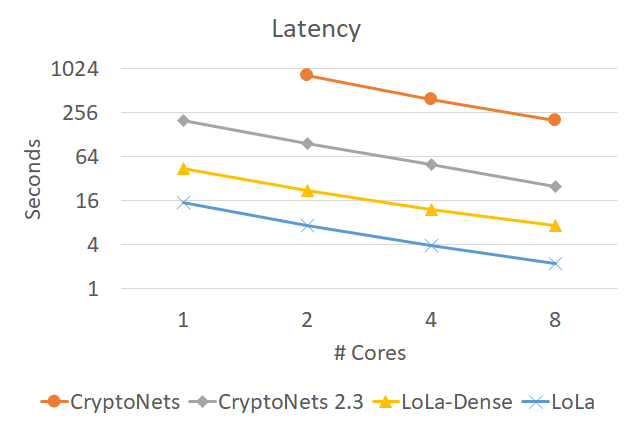
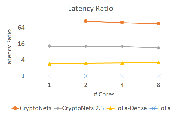
Figure 2: Left: latency of the different network implementations for the MNIST task with respect to the number of available cores. Right: ratio between the latency of each solution and the latency of LoLa

Appendix C Lola-Dense

LoLa-Dense uses the same network layout as CryptoNets (see Figure 3) and has accuracy of $98.95\%$. However, it is implemented differently: the input to the network is a single dense message where the pixel values are mapped to coordinates in the encoded vector line after line . The first step in processing this message is breaking it into 25 messages corresponding to the 25 pixels in the convolution map to generate a convolution representation. Creating each message requires a single vector multiplication. This is performed by creating 25 masks. The first mask is a vector of zeros and ones that corresponds to a matrix of size $28\times 28$ such that a one is in the $\left(i,j\right)$ coordinate if the $i,j$ pixel in the image appears as the upper left corner of the $5\times 5$ window of the convolution layer. Multiplying point-wise the input vector by the mask creates the first message in the convolution representation hybrided with the interleaved representation. Similarly the other messages in the convolution representation are created. Note that all masks are shifts of each other which allows using the convolution representation-row major multiplication to implement the convolution layer. To do that, think of the $25$ messages as a matrix and the weights of a map of the convolution layer as a sparse vector. Therefore, the outputs of the entire map can be computed using $25$ multiplications (of each weight by the corresponding vector) and $24$ additions. Note that there are $169$ windows and all of them are computed simultaneously. However, the process repeats 5 times for the $5$ maps of the convolution layer.

The result of the convolution layer are $5$ messages, each one of them contains $169$ results. They are united into a single vector by rotating the messages such that they will not have active values in the same locations and summing the results. At this point, a single message holds all the $845$ values ($169$ windows $\times 5$ maps). This vector is squared, using a single multiplication operation, to implement the activation function that follows the convolution layer. This demonstrates one of the main differences between CryptoNets and LoLa; In CryptoNets, the activation layer requires $845$ multiplication operations, whereas in LoLa it is a single multiplication. Even if we add the manipulation of the vector to place all values in a single message, as described above, we add only $4$ rotations and $4$ additions which are still much fewer operations than in CryptoNets.

Next, we apply a dense layer with $100$ maps. LoLa-Dense uses messages of size $n=16384$ where the $845$ results of the previous layer, even though they are in interleaving representation, take fewer than $1024$ dimensions. Therefore, $16$ copies are stacked together which allows the use of the Stacked vector – Row Major multiplication method. This allows computing $16$ out of the $100$ maps in each operation and therefore, the entire dense layer is computed in 7 iterations resulting in $7$ interleaved messages. By shifting the $i^{\text{th}}$ message by $i-1$ positions, the active outputs in each of the messages are no longer in the same position and they are added together to form a single interleaved message that contains the $100$ outputs. The following square activation requires a single point-wise-multiplication of this message. The final dense layer is applied using the Interleaved vector – Row Major method to generate $10$ messages, each of which contains one of the $10$ outputs.

Overall, applying the entire network takes only $7.2$ seconds on the same reference hardware which is $34.7\times$ faster than CryptoNets and $3.4\times$ faster than CryptoNets 2.3.

Figure 3: The structure of the network used for MNIST classification.

Layer	Input size	Representation	LoLa-Dense Operation
$5\times 5$ convolution layer	$1\times 784$	dense	mask input to create 25 messages
	$25\times 169$	convolution-interleave	convolution vector – row major mult’
	$5\times 169$	interleave	combine 5 messages into one
square layer	$1\times 845$	interleave	square
dense layer	$1\times 845$	interleave	stack 16 copies
	$1\times 13520$	stacked-interleave	stacked vector – row major mult’
	$7\times 16$	interleave	combine 7 messages into one
square layer	$1\times 100$	interleave	square
dense layer	$1\times 100$	interleave	interleaved vector – row major
output layer	$10\times 1$	sparse

Table 3: Message size, message representation and operations in each layer of the LoLa-Dense inference solution on MNIST. The input size format is number of vectors $\times$ dimension

Appendix D Secure CIFAR

The neural network used has the following layout: the input is a $3\times 32\times 32$ image (i) $3\times 3$ linear convolution with stride of $\left(1,1\right)$ and 128 output maps, (ii) $2\times 2$ average pooling with $\left(2,2\right)$ stride (iii) $3\times 3$ convolution with $\left(1,1\right)$ stride and 83 maps (iv) Square activation (v) $2\times 2$ average pooling with $\left(2,2\right)$ stride (vi) $3\times 3$ convolution with $\left(1,1\right)$ stride and 163 maps (vii) Square activation (vii) $2\times 2$ average pooling with stride $\left(2,2\right)$ (viii) fully connected layer with $1024$ outputs (ix) fully connected layer with $10$ outputs (x) softmax. ADAM was used for optimization Kingma & Ba (2014) together with dropouts after layers (vii) and (viii). We use zero-padding in layers (i) and (vii). See Figure 4 for an illustration of the network.

For inference, adjacent linear layers were collapsed to form the following structure: (i) $8\times 8\times 3$ convolutions with a stride of $\left(2,2,0\right)$ and 83 maps (ii) square activation (iii) $6\times 6\times 83$ convolution with stride $\left(2,2,0\right)$ and 163 maps (iv) square activation (v) dense layer with $10$ output maps. See Figure 5 for an illustration.

Figure 4: The structure of the network used for CIFAR classification.

Figure 5: The structure of the network used for CIFAR classification after collapsing adjacent layers.

Appendix E CalTech-101

Table 4 shows the different data representations when using the method proposed for private inference on the CalTech-101 dataset using deep representations.

Layer	Input size	Output format	Description
Preprocess	$200\times 300$	dense	apply convolution layers from Alex-Net
Encryption	$4096$	dense	image is encrypted into $1$ message
dense layer	$101$	sparse	dense-vector row major multiplication

Table 4: Data representation changes for CalTech 101 task

References

- Albrecht et al. (2018) Martin Albrecht, Melissa Chase, Hao Chen, Jintai Ding, Shafi Goldwasser, Sergey Gorbunov, Jeffrey Hoffstein, Kristin Lauter, Satya Lokam, Daniele Micciancio, et al. Homomorphic encryption standard. 2018.
- Badawi et al. (2018) Ahmad Al Badawi, Jin Chao, Jie Lin, Chan Fook Mun, Sim Jun Jie, Benjamin Hong Meng Tan, Xiao Nan, Khin Mi Mi Aung, and Vijay Ramaseshan Chandrasekhar. The alexnet moment for homomorphic encryption: Hcnn, the first homomorphic cnn on encrypted data with gpus. arXiv preprint arXiv:1811.00778, 2018.
- Boemer et al. (2018) Fabian Boemer, Yixing Lao, and Casimir Wierzynski. ngraph-he: A graph compiler for deep learning on homomorphically encrypted data. arXiv preprint arXiv:1810.10121, 2018.
- Bourse et al. (2017) Florian Bourse, Michele Minelli, Matthias Minihold, and Pascal Paillier. Fast homomorphic evaluation of deep discretized neural networks. Technical report, Cryptology ePrint Archive, Report 2017/1114, 2017.
- Brakerski & Vaikuntanathan (2014) Zvika Brakerski and Vinod Vaikuntanathan. Efficient fully homomorphic encryption from (standard) lwe. SIAM Journal on Computing, 43(2):831–871, 2014.
- Brakerski et al. (2014) Zvika Brakerski, Craig Gentry, and Vinod Vaikuntanathan. (leveled) fully homomorphic encryption without bootstrapping. ACM Transactions on Computation Theory (TOCT), 6(3):13, 2014.
- Chen et al. (2018) Guoxing Chen, Sanchuan Chen, Yuan Xiao, Yinqian Zhang, Zhiqiang Lin, and Ten H Lai. Sgxpectre attacks: Leaking enclave secrets via speculative execution. arXiv preprint arXiv:1802.09085, 2018.
- Cheon et al. (2017) Jung Hee Cheon, Andrey Kim, Miran Kim, and Yongsoo Song. Homomorphic encryption for arithmetic of approximate numbers. In International Conference on the Theory and Application of Cryptology and Information Security, pp. 409–437. Springer, 2017.
- Chou et al. (2018) Edward Chou, Josh Beal, Daniel Levy, Serena Yeung, Albert Haque, and Li Fei-Fei. Faster cryptonets: Leveraging sparsity for real-world encrypted inference. arXiv preprint arXiv:1811.09953, 2018.
- Dowlin et al. (2016) Nathan Dowlin, Ran Gilad-Bachrach, Kim Laine, Kristin Lauter, Michael Naehrig, and John Wernsing. Cryptonets: Applying neural networks to encrypted data with high throughput and accuracy. In International Conference on Machine Learning, pp. 201–210, 2016.
- Dowlin et al. (2017) Nathan Dowlin, Ran Gilad-Bachrach, Kim Laine, Kristin Lauter, Michael Naehrig, and John Wernsing. Manual for using homomorphic encryption for bioinformatics. Proceedings of the IEEE, 105(3):552–567, 2017.
- Fan & Vercauteren (2012) Junfeng Fan and Frederik Vercauteren. Somewhat practical fully homomorphic encryption. IACR Cryptology ePrint Archive, 2012:144, 2012.
- Fei-Fei et al. (2006) Li Fei-Fei, Rob Fergus, and Pietro Perona. One-shot learning of object categories. IEEE transactions on pattern analysis and machine intelligence, 28(4):594–611, 2006.
- Gentry (2009) Craig Gentry. Fully homomorphic encryption using ideal lattices. In STOC, volume 9, pp. 169–178, 2009.
- Goldreich et al. (1987) Oded Goldreich, Silvio Micali, and Avi Wigderson. How to play any mental game. In Proceedings of the nineteenth annual ACM symposium on Theory of computing, pp. 218–229. ACM, 1987.
- He et al. (2016) Kaiming He, Xiangyu Zhang, Shaoqing Ren, and Jian Sun. Deep residual learning for image recognition. In Proceedings of the IEEE conference on computer vision and pattern recognition, pp. 770–778, 2016.
- Juvekar et al. (2018) Chiraag Juvekar, Vinod Vaikuntanathan, and Anantha Chandrakasan. Gazelle: A low latency framework for secure neural network inference. arXiv preprint arXiv:1801.05507, 2018.
- Kingma & Ba (2014) Diederik P Kingma and Jimmy Ba. Adam: A method for stochastic optimization. arXiv preprint arXiv:1412.6980, 2014.
- Koruyeh et al. (2018) Esmaeil Mohammadian Koruyeh, Khaled Khasawneh, Chengyu Song, and Nael Abu-Ghazaleh. Spectre returns! speculation attacks using the return stack buffer. In 12th USENIX Workshop on Offensive Technologies (WOOT 18). USENIX Association, 2018.
- Krizhevsky & Hinton (2009) Alex Krizhevsky and Geoffrey Hinton. Learning multiple layers of features from tiny images. Technical report, Citeseer, 2009.
- Krizhevsky et al. (2012) Alex Krizhevsky, Ilya Sutskever, and Geoffrey E Hinton. Imagenet classification with deep convolutional neural networks. In Advances in neural information processing systems, pp. 1097–1105, 2012.
- LeCun et al. (2010) Yann LeCun, Corinna Cortes, and Christopher JC Burges. Mnist handwritten digit database. at&t labs, 2010.
- Makri et al. (2019) Eleftheria Makri, Dragos Rotaru, Nigel P Smart, and Frederik Vercauteren. Epic: efficient private image classification (or: learning from the masters). In Cryptographers Track at the RSA Conference, pp. 473–492. Springer, 2019.
- McKeen et al. (2013) Frank McKeen, Ilya Alexandrovich, Alex Berenzon, Carlos V Rozas, Hisham Shafi, Vedvyas Shanbhogue, and Uday R Savagaonkar. Innovative instructions and software model for isolated execution. HASP@ ISCA, 10, 2013.
- Riazi et al. (2018) M Sadegh Riazi, Christian Weinert, Oleksandr Tkachenko, Ebrahim M Songhori, Thomas Schneider, and Farinaz Koushanfar. Chameleon: A hybrid secure computation framework for machine learning applications. In Proceedings of the 2018 on Asia Conference on Computer and Communications Security, pp. 707–721. ACM, 2018.
- Sanyal et al. (2018) Amartya Sanyal, Matt J Kusner, Adrià Gascón, and Varun Kanade. Tapas: Tricks to accelerate (encrypted) prediction as a service. arXiv preprint arXiv:1806.03461, 2018.
- Simonyan & Zisserman (2014) Karen Simonyan and Andrew Zisserman. Very deep convolutional networks for large-scale image recognition. arXiv preprint arXiv:1409.1556, 2014.
- Tajbakhsh et al. (2016) Nima Tajbakhsh, Jae Y Shin, Suryakanth R Gurudu, R Todd Hurst, Christopher B Kendall, Michael B Gotway, and Jianming Liang. Convolutional neural networks for medical image analysis: Full training or fine tuning? IEEE transactions on medical imaging, 35(5):1299–1312, 2016.
- Tramer & Boneh (2018) Florian Tramer and Dan Boneh. Slalom: Fast, verifiable and private execution of neural networks in trusted hardware. arXiv preprint arXiv:1806.03287, 2018.
- Yao (1982) Andrew C Yao. Protocols for secure computations. In Foundations of Computer Science, 1982. SFCS’08. 23rd Annual Symposium on, pp. 160–164. IEEE, 1982.
- Yosinski et al. (2014) Jason Yosinski, Jeff Clune, Yoshua Bengio, and Hod Lipson. How transferable are features in deep neural networks? In Advances in neural information processing systems, pp. 3320–3328, 2014.