Magnetically tunable multi-band near-field radiative heat transfer between two graphene sheets

Abstract

Near-field radiative heat transfer (NFRHT) is strongly related with many applications such as near-field imaging, thermos-photovoltaics and thermal circuit devices. The active control of NFRHT is of great interest since it provides a degree of tunability by external means. In this work, a magnetically tunable multi-band NFRHT is revealed in a system of two suspended graphene sheets at room temperature. It is found that the single-band spectra for B=0 split into multi-band spectra under an external magnetic field. Dual-band spectra can be realized for a modest magnetic field (e.g., B=4 T). One band is determined by intra-band transitions in the classical regime, which undergoes a blue shift as the chemical potential increases. Meanwhile, the other band is contributed by inter-Landau-level transitions in the quantum regime, which is robust against the change of chemical potentials. For a strong magnetic field (e.g., B=15 T), there is an additional band with the resonant peak appearing at near-zero frequency (microwave regime), stemming from the magneto-plasmon zero modes. The great enhancement of NFRHT at such low frequency has not been found in any previous systems yet. This work may pave a way for multi-band thermal information transfer based on atomically thin graphene sheets.

I Introduction

The management of near-field radiative heat transfer (NFRHT) has promising applications in energy conversion Fio:18 ; Zha:17 ; Bas:09 and information processing Abd:17 ; Abd:16a . Thanks to the tunneling of evanescent waves (e.g., surface plasmon polaritions (SPPs) Jou:05 ; Bor:15 , surface phonon polaritions (SPhPs) She:09 ; Son:15 ), the radiative heat flux can exceed the blackbody limit by several orders of magnitude for nanoscale separation Vol:07 ; liu:15 . The field of NFRHT grows rapidly in recent years Cue:18 . Particularly, the thermal analogy of the electronic devices Abd:17 , i.e.,thermotronics, provides a new possibility for information processing. The fast thermal photon generated from NFRHT is an attractive information carrier compared with its counterpart of the slow phonon (heat conduction) Li:12 . Up to now, the proposals for fundamental circuit elements such as thermal logic gates Abd:16a , thermal rectifiers Ote:10 , thermal memory Kub:14 ; Ito:16 , thermal transistors Abd:14 have been reported. Despite great progress in thermal circuit devices, the active and fast control of NFRHT is still highly desired for thermal information processing.

Recently, several strategies for active control of NFRHT have been proposed Ili:18 ; Hua:14 ; Cui:13 ; Kou:18 ; Abd:16b ; Zhu:16 ; Eke:18 ; Mon:15 ; Van:11 ; Van:12 ; Gha:18 . For instance, one can tune the NFRHT by external electric gating in 2D materials Ili:18 and ferroelectric materials Hua:14 . Or one can use optical pump, i.e., photo-excitation, to control NFRHT in chiral meta-materials Cui:13 and semiconductors Kou:18 . In addition, one can actively control NFRHT through an external magnetic field Abd:16b ; Zhu:16 ; Eke:18 ; Mon:15 . Examples such as near-field thermal Hall effect Abd:16b , persistent directional heat current Zhu:16 , anisotropic thermal magnetoresistance  Eke:18 , and thermal modulation Mon:15 were reported. Other schemes such as temperature control in phase-change materials Van:11 ; Van:12 , and mechanical strain Gha:18 are also investigated. However, previous studies of various strategies for active control of NFRHT have been focused on enhancing or suppressing the total heat flux. Little attention was paid on the control of multi-band spectral bands. Inspired by the multi-band devices in telecommunications, a controllable thermal transfer system with multi-band spectra could be significant for the development of thermal information processing.

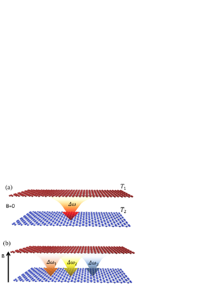
Figure 1: (color online) Schematic view of near-field radiative heat transfer between two suspended graphene sheets in free space. The upper sheet with higher temperature ($T_{1}$) radiates electromagnetic waves to the bottom one with lower temperature ($T_{2}$). (a) The spectrum of radiative heat flux is single-band in the absence of an external magnetic field. (b) The spectrum becomes multi-band under a sufficient strong magnetic field.

In order to realize multi-band NFRHT, one straight scheme is to design a system with multiple frequency-separated surface modes. The SPPs can be modulated under an external magnetic field (or named magneto-plasmon) Hu:15 . The multi-band dispersions, i.e., energy gaps appear in the dispersion relationship, can be found in magneto-plasmon of doped semiconductors Bri:72 and graphene Fer:12 ; Hu:14 . Compared with the doped semiconductors, graphene is only one-atom thick Gei:07 . Besides, the cyclotron energy of graphene, characterized by the quantized Landau level (LL) transitions Goe:11 , can be much larger than those of semiconductors under the same magnetic field. The magneto-plasmon of graphene lies in Terahertz and far infrared frequencies Fer:12 ; Hu:14 , which guarantees a high-efficiency thermal excitation at room temperature.

In this work, we investigate the NFRHT between two parallel graphene sheets under a perpendicular magnetic field. It is found that the single-band spectrum for B=0 can be split into multi-band spectra under an external magnetic field at room temperature. The multi-band spectra are determined by the LL transitions of graphene, which show interesting properties due to thermal fluctuation. For a modest magnetic field (e.g., B=4 T), dual-band spectra can be realized, contributed from intra-band and inter-band LL transitions, respectively. Interestingly, the latter one is quite robust against the change of chemical potential. On the other hand, triple-band spectra can be found under a strong magnetic field (e.g., B=15 T). Remarkably, there is an additional band with the resonant peak appearing at near-zero frequency. The great enhancement of NFRHT at such low frequency is attributed to the magneto-plasmon zero modes. Finally, the properties of multi-band NFRHT due to the scattering rate, separation distance and substrate effect are discussed at the end.

II Theories for magnetically tunable NFRHT

The system considered in this work is depicted in Fig. 1. Two parallel graphene sheets are suspended in free space with a separation distance $d$. The temperatures for the upper and bottom sheets are respectively $T_{1}$ and $T_{2}$. The value of the perpendicular magnetic field B can be tuned though external control. In this work, we consider the magnetic field $\text{B}<$17 T, where the Zeeman splitting is negligible Zha:06 . The magneto-optical conductivity of graphene is given by a tensor Gus:07 ; Fer:11 :

$$\left(\begin{array}[]{cc}\sigma_{xx}&\sigma_{xy}\\ \sigma_{yx}&\sigma_{yy}\end{array}\right)=\left(\begin{array}[]{cc}\sigma_{L}&\sigma_{H}\\ -\sigma_{H}&\sigma_{L}\end{array}\right),$$ (1)

where the subscripts $L$ and $H$ represent respectively the longitudinal and Hall conductivities, and they can be written in compact forms  Fer:11 :

$$\sigma_{L(H)}(\omega,B)=g_{s}g_{v}\frac{e^{2}}{4h}\underset{n\neq m}{\overset{\infty}{\sum}}\frac{\Xi_{L(H)}^{nm}}{i\Delta_{nm}}\frac{n_{F}(E_{n})-n_{F}(E_{m})}{\hbar\omega+\Delta_{nm}+i\Gamma_{nm}},$$ (2)

where $g_{s}$=$g_{v}$=2 are respectively the spin and valley degeneracy factors, $e$ is the charge of an electron, $h$ is the plank constant, $\Gamma_{nm}$ is the scattering rate (the broadening of LLs), $n_{F}(E_{n})=1/[1+\exp(E_{n}-\mu_{c})/k_{B}T]$ is the Fermi-Dirac distribution, and $\mu_{c}$ is the chemical potential, $k_{B}$ is the Boltzmann constant, $\Delta_{nm}=E_{n}-E_{m}$ is the LL energy transition with $n$, $m$=0, $\pm 1$, $\pm 2$… are the Landau indices, $E_{n}=$sign$(n)[\hbar v_{F}/l_{B}]\sqrt{2|n|}$ is the energy of the $n$-th LL, $v_{F}$=$10^{6}$ m/s is the Fermi velocity, $l_{B}\equiv\sqrt{\hbar/(eB)}$ is the magnetic length, and the auxiliary functions are given by:

$$\Xi_{L}^{nm} = \frac{\hbar^{2}v_{F}^{2}}{l_{B}^{2}}(1+\delta_{m,0}+\delta_{n,0})\delta_{|m|-|n|,\pm 1},$$

$$\Xi_{H}^{nm} = i\Xi_{L}^{nm}(\delta_{|m|,|n|-1}+\delta_{|m|-1,n}),$$ (3)

which are determined by the selection rule of LL transitions. The radiative heat flux between two graphene sheets under an external magnetic field can be calculated based on the fluctuation-dissipation theory  Bie:11 :

$$\left\langle S\right\rangle=\frac{1}{(2\pi)^{2}}\int_{0}^{\infty}\int_{0}^{\infty}\xi(\omega,q)q\text{d}q[\Theta(\omega,T_{1})-\Theta(\omega,T_{2})]\text{d}\omega,$$ (4)

where $\Theta(\omega,T)=\hbar\omega/(\exp(\hbar\omega/k_{B}T)-1)$ is the average energy of a Planck’s oscillator for angular frequency $\omega$ at temperature $T$, and $q$ is the wavevector parallel to the surface planes, $\xi(\omega,q)$ is the energy transmission coefficient, which is expressed as follows:

$$\xi(\omega,q)$$

$$= \left\{\begin{array}[]{c}\text{Tr}[(\mathbf{I}-\mathbf{R}_{2}^{\dagger}\mathbf{R}_{2})\mathbf{D}^{12}(\mathbf{I}-\mathbf{R}_{1}^{\dagger}\mathbf{R}_{1})\mathbf{D}^{12\dagger}],\\ \text{Tr}[(\mathbf{R}_{2}^{\dagger}-\mathbf{R}_{2})\mathbf{D}^{12}(\mathbf{R}_{1}^{\dagger}-\mathbf{R}_{1})\mathbf{D}^{12\dagger}]e^{-2|\gamma|d},\end{array}\right.\begin{array}[]{c}q<k_{0}\\ q>k_{0}\end{array}$$

where $\gamma=\sqrt{k_{0}^{2}-q^{2}}$ is the vertical wavevector with $k_{0}=\omega/c$ being the wavevector in vacuum, $\mathbf{D}^{12}=(\mathbf{I}-\mathbf{R}_{1}\mathbf{R}_{2}e^{2i\gamma d})^{-1}$ and $\mathbf{R}_{j}$ ($j$=1, 2) is the $2\times 2$ reflection matrix for the $j$-th graphene sheet, having the form:

$$\mathbf{R}_{j}=\left(\begin{array}[]{cc}r_{j}^{ss}&r_{j}^{sp}\\ r_{j}^{ps}&r_{j}^{pp}\end{array}\right),$$ (9)

where the superscripts $s$ and $p$ represent respectively the polarizations of transverse electric ($\mathbf{TE}$) and transverse magnetic ($\mathbf{TM}$) modes. The matrix element $r^{\alpha\beta}$ ($\alpha,\beta$ = $s,p$) represents the reflection coefficient for an incoming $\alpha$-polarized plane wave being reflected into an outgoing $\beta$-polarized wave. For a suspended graphene sheet under a perpendicular magnetic field, the reflection coefficients are given analytically as follows Kot:17 ; Tse:12 :

$$r^{ss} = -\frac{2k_{0}^{2}\overline{\sigma}_{L}+k_{0}\gamma(\overline{\sigma}_{L}^{2}+\overline{\sigma}_{H}^{2})}{4k_{0}\gamma+(2\gamma^{2}+2k_{0}^{2})\overline{\sigma}_{L}+k_{0}\gamma(\overline{\sigma}_{L}^{2}+\overline{\sigma}_{H}^{2})},$$

$$r^{pp} = -\frac{2\gamma^{2}\overline{\sigma}_{L}+k_{0}\gamma(\overline{\sigma}_{L}^{2}+\overline{\sigma}_{H}^{2})}{4k_{0}\gamma+(2\gamma^{2}+2k_{0}^{2})\overline{\sigma}_{L}+k_{0}\gamma(\overline{\sigma}_{L}^{2}+\overline{\sigma}_{H}^{2})},$$ (10)

$$r^{ps} = -r^{sp}=\frac{2k_{0}\gamma\overline{\sigma}_{H}}{4k_{0}\gamma+(2\gamma^{2}+2k_{0}^{2})\overline{\sigma}_{L}+k_{0}\gamma(\overline{\sigma}_{L}^{2}+\overline{\sigma}_{H}^{2})},$$

where the elements of conductivity tensor are normalized by the free-space impedance $\sqrt{\mu_{0}/\varepsilon_{0}}$. Note that the denominator in all reflection coefficients is the same. By setting this denominator to be zero and the loss term $\Gamma$=0, the dispersion of magneto-plasmon in single graphene sheet can be obtained.

We now consider the NFRHT in the low frequency limit $\omega\rightarrow 0$, where the normalized conductivities Im$\overline{\sigma}_{L}$, Im$\overline{\sigma}_{H}\rightarrow 0$ and Re$\overline{\sigma}_{L}$, Re$\overline{\sigma}_{H}\ll 1$. For very large wave-vector $q\gg k_{0}$, i.e., $|\gamma|\gg k_{0}$, only the reflection coefficient $r^{pp}$ plays an important role, and it can be simplified as:

$$r^{pp}=-\frac{iq\overline{\sigma}_{L}}{2k_{0}+iq\overline{\sigma}_{L}}.$$ (11)

The pole of the denominator (real part) appears at $\omega$=0, which corresponds to a magneto-plasmon zero-mode. The NFRHT is proportional to Im$[r^{pp}]$  Ili:18 , where it has the expression Im[$r^{pp}$]=-2$k_{0}/(q\mathrm{Re}\overline{\sigma}_{L})$. For a strong magnetic field, the longitudinal conductivity of graphene, i.e., the term $\mathrm{Re}\overline{\sigma}_{L}$, can be diminished with orders of magnitude compared with the non-magnetic configuration, based on the calculations of Eq. (2). As a result, the NFRHT at near-zero frequency can be enhanced greatly due to the magneto-plasmon zero modes, which is an important finding in our work. It should be pointed out that the magneto-plasmon zero modes in 2D electron gas systems were also demonstrated in the Ref. Jin:16 .

III Results and discussions

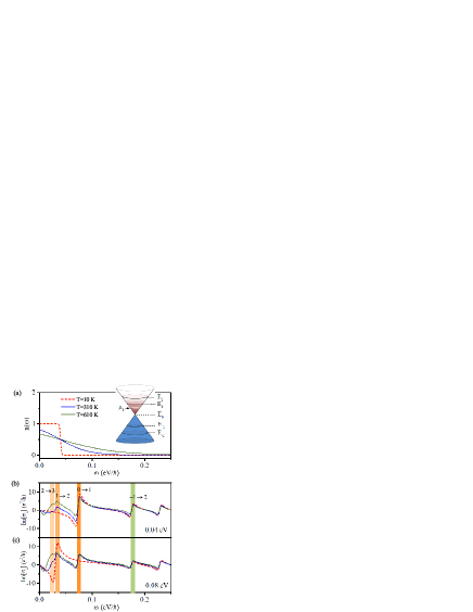
Figure 2: (color online) (a) The Fermi-Dirac distribution of graphene for different temperatures. The inset illustrates the band structure of a graphene sheet with chemical potential $\mu_{c}$ below the first LL. The imaginary part of longitudinal conductivity Im[$\sigma_{L}$] for (b) $\mu_{c}$=0.04 eV and (c) $\mu_{c}$=0.08 eV. The shaded regimes in (b) and (c) indicate the peaks of conductivity contributed by different LL transitions. The scattering rate is set to be a constant with $\Gamma_{nm}$=$\Gamma$= 4 meV. The external magnetic field B=4 T, and the first LL E${}_{1}\sim$0.07 eV.

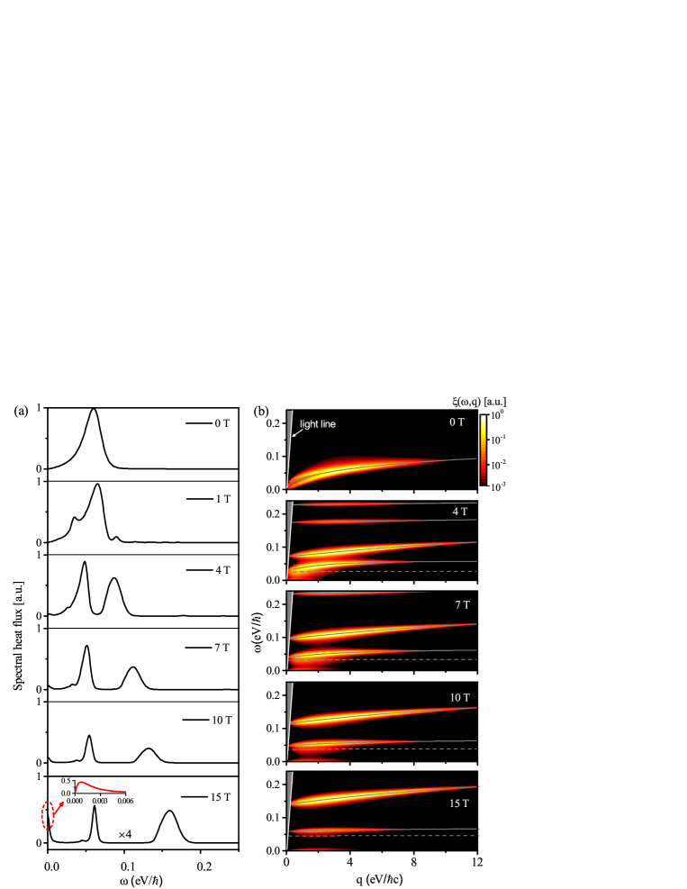
Figure 3: (color online) (a) Spectral heat flux and (b) transmission coefficients(log scale) for two parallel graphene sheets under different values of magnetic field. The inset in (a) shows the spectrum near-zero frequency for B=15 T. In (b), the white line illustrates the light line q=$\omega$/c, and the gray lines represent the corresponding dispersions of magneto-plasmon for single graphene sheet. The dashed gray lines stand for the dispersions generated from the intra-band transition E${}_{2}\rightarrow$E₃. We set the chemical potential for two graphene sheets $\mu_{c1}=\mu_{c2}$=0.08 eV, the scattering rate $\Gamma$=4 meV, the high temperature $T_{1}$=310 K, the low temperature $T_{2}$=$T_{1}$-10 K, and the separation distance $d$=100 nm.

To understand the magneto-plasmon of graphene at high temperature, we firstly inspect the Fermi-Dirac distribution $n(\omega)$ in Fig. 2(a). Clearly, $n(\omega)$ is a good quantum number at low temperature 10 K, whereas it becomes partially occupied at high temperatures 310 K and 610 K, due to the thermal fluctuation. The inset schematically shows the band structure of graphene with quantized LLs and Fermi-Dirac distribution of electron at high temperatures. The long-decay tails of $n(\omega)$ enable multiple intra-band LL transitions take place (such as E${}_{1}\rightarrow$E₂, E${}_{2}\rightarrow$E₃) even though $\mu_{c}$ is smaller than the first LL E₁.

We are interest in the imaginary part of longitudinal conductivity, i.e., Im[$\sigma_{L}$], as the magneto-plasmon of graphene is mainly determined by this component Fer:12 . The magneto-plasmon of graphene are confirmed strongly when Im[$\sigma_{L}$] is a positive number, providing a capability for the enhancement of NFRHT. The comb-like curves of Im[$\sigma_{L}$] are shown in Figs. 2(b) and 2(c), where the magnetic field B =4 T, and the first LL E${}_{1}\sim$0.07 eV. The values of chemical potential of graphene are controllable though external electric gating Gri:12 . For chemical potential $\mu_{c}$=0.04 eV$<$ E₁, there is no intra-band transition for temperature 10 K. However, multiple intra-band transitions (mainly E${}_{1}\rightarrow$E₂ and E${}_{2}\rightarrow$E₃) take place for 310 K and 610 K at low frequency, which differ considerably from those of 10 K. The conductivity Im[$\sigma_{L}$] with chemical potential located between E₁ and E₂ is shown in Fig. 2(c) for $\mu_{c}$=0.08 eV. At this time, the conductivity at low temperature 10 K is somewhat different from those of $\mu_{c}$=0.04 eV. Now there is an intra-band transition E${}_{1}\rightarrow$E₂, whereas the inter-band transition E${}_{0}\rightarrow$E₁ is absent. By contrast, both multiple intra-band (E₁$\rightarrow$ E₂, E₂ $\rightarrow$ E₃) and inter-band (E₀ $\rightarrow$ E₁) LL transitions still exist at temperatures 310 K and 610 K. However, the dependence of Im[$\sigma_{L}$] on the temperature becomes small at high frequency. This is because the energies of inter-band LLs transitions are much higher than those of thermal fluctuation (e.g, $k_{B}T\sim$0.027 eV for 310 K).

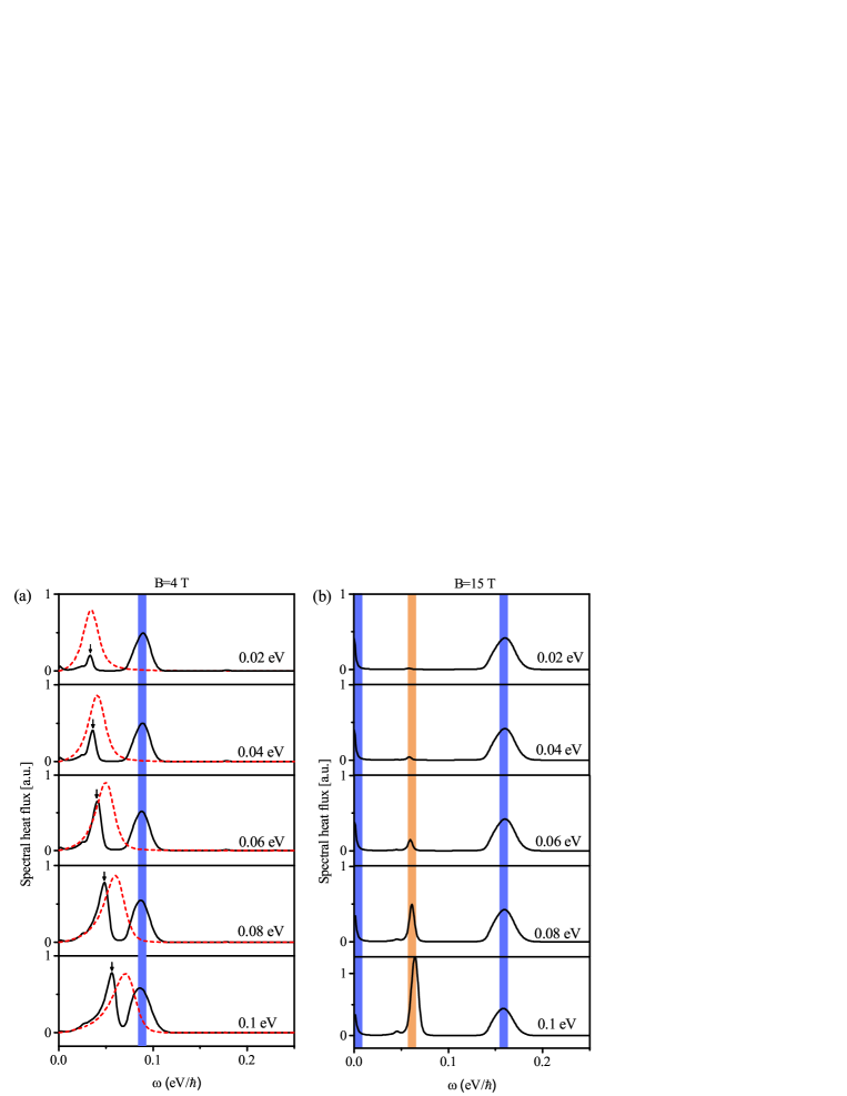
Figure 4: (color online) Spectral heat flux via chemical potential ($\mu_{c1}$=$\mu_{c2}$) for (a) B=4 T. The red dashed curves represent the corresponding spectra for B=0, where the resonant peaks have a blue shift as the chemical potential increases. (b) B=15 T. The middle spectral band (the orange shaded regime) changes dramatically with increasing the chemical potential. However, the spectral bands marked by the blue shaded regimes in (a) and (b) are almost unchanged, showing a robust feature.

Figure 3(a) shows the spectra of radiative heat flux under different magnetic fields. In the absence of magnetic field, the spectral heat flux is single-band as reported in Ref. Ili:12 . Compared with the non-magnetic configuration, the spectra are modulated correspondingly after the magnetic field is turned on. For instance, there are some small peaks for B=1 T. As the magnetic field increases further, dual-band spectra can be found for B=4 T, 7 T and 10 T. Overall, the peaks of the two spectral bands undergo a blue shift and the energy gap between these two peaks enlarges as the magnetic field increases. For a strong magnetic field B=15 T, triple-band spectrum can be seen clearly. In addition to those two spectral bands mentioned above, there is a remarkable band close to zero frequency, and it is plotted in the inset for clarity. The resonant peak for this low-frequency band appears at 0.8 meV ($\sim$200 GHz), which lies in the microwave regime. The great enhancement of NFRHT in such low frequency has not been revealed in any previous systems before. Although the amplitude of spectrum has been multiplied 4 times for B=15 T, the radiative heat flux can still exceed the black body limit over 40 times, which is large enough for potential applications in triple-band thermal devices.

To clarify the origin of multi-band spectra, we plot of transmission coefficient $\xi(\omega,q)$ below the light line in Fig. 3(b). The large wave-vector $q\gg k_{0}$ indicates that the NFRHT is mainly contributed by the evanescent waves. Specifically, the transmission coefficient for B=0 is continuous over the frequency regime, resulting in a single-band spectrum. By contrast, the transmission coefficients for B=4 T, 7 T, 10 T and 15 T turn out to be frequency separated configurations, leading to multi-band spectra. Interestingly, there is an extraordinary band started from zero frequency, which is generated from magneto-plasmon zero modes as mentioned before. This band can be prominently seen, especially for strong magnetic field B=10 T and 15 T. It is worth mentioning that the transmission coefficient $\xi(\omega,q)$ due to high-order LL transitions can be seen as well for B=4 T and 7 T with $\omega>$0.15 eV/$\hbar$. However, the contribution of high-order LL transitions to the NFRHT is very small, due to the fast decay of the term $\Theta(\omega,T)$ at high frequency. For comparison, the dispersions of magneto-plasmon in single graphene sheet are given correspondingly. It is found that the dispersions turn out to be a series of branches at the presence of magnetic field, which agree well with transmission coefficient $\xi(\omega,q)$. Since the transmission coefficient $\xi(\omega,q)$ generated from intra-band transition E${}_{2}\rightarrow$E₃ is very small, the corresponding dispersions are plotted in the dashed gray lines to indicate their insignificance in NFRHT.

The chemical potential of graphene is an important parameter, which can be tuned greatly by electrical gating. The spectral heat flux via different chemical potential are shown in Figs. 4(a) and 4(b). For B= 4 T, there are two primary spectral bands. The first primary band (marked by the black arrows) has a relative poor excitation when the chemical potential is small (e.g., $\mu_{c}=0.02$ eV). As the chemical potential increases, however, the magnitudes of this band increase and the spectral peaks have a blue shift. This evolution is attributed to the properties of intra-band transition. On the other hand, the second band (marked by blue shaded regime) is contributed by the inter-band LL transition (E₀$\rightarrow$E₁). Surprisingly, the magnitude and line-shape of this spectral band have little change as chemical potential increases from 0.02 eV to 0.1 eV, showing a robust feature. For comparison, the spectral heat flux for B=0 are given by the red dashed lines. The resonant peaks of spectra for B=0 undergo a blue shift when the chemical potential increases, indicating a trivial feature contributed by the intra-band transitions. For a strong magnetic field B=15 T, the first and the third spectral bands (blue shaded regimes) are robust against the change of chemical potential as well. Interestingly, the middle spectral band (orange shaded regimes) contributed by intra-band transitions is suppressed strongly at low doping 0.02 eV and 0.04 eV. This is attributed to high energy of first LL (E₁$\sim$ 0.14 eV for 15 T), resulting in low probability of intra-band transition. As expected, the magnitude of the middle spectrum-band increases with the chemical potential, and it has the same order with the two side bands when the chemical potential $\mu_{c}\sim$0.08 eV. Thus, triple-band radiative heat transfer can be realized for suitable tuning of chemical potential under a strong magnetic field. As the chemical potential increases further to $\mu_{c}$=0.1 eV, the middle band is dominant.

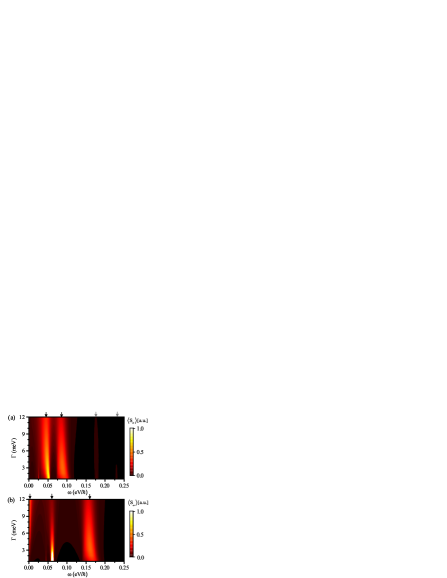
Figure 5: (color online) Contour plots of spectral heat flux for different scattering rate. (a) B=4 T, and (b) B=15 T. The black arrows indicates the primary bands, and the gray arrows represent secondary bands contributed from high order LL transitions. The chemical potential, temperatures and separation distance are kept the same as those in Fig. 3.

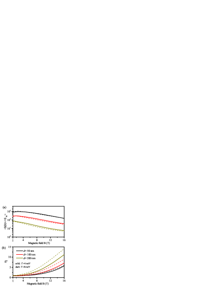
Figure 6: (color online) (a) The radiative heat flux as a function of magnetic field, normalized by blackbody limit. (b)The modulation of radiative heat flux in the presence of magnetic field, defined as $\eta=\left\langle S(\text{B}=0)\right\rangle$/$\left\langle S(\text{B})\right\rangle$. The solid and dash curves represent the scattering rate $\Gamma$=4 meV and 8 meV, respectively. The chemical potential and temperatures are kept the same as those in Fig. 3.

To study in a more general way, the scattering rate is assumed to be a constant but within a typical range $\Gamma\in$ [1, 12]meV (see, e.g., Fer:12 ; Cra:11 ). The contour plots of spectral heat flux are shown in Figs. 5(a) and 5(b). For B=4 T, the peak frequencies of the two primary bands indicated by the black arrows almost do not changed as $\Gamma$ increase from 1 meV to 12 meV. Although the magnitude of spectral band become smaller for large scattering rate, the two primary bands are still dominant. The contour plot of spectral heat flux for B=15 T is shown in Fig. 5(b). Again, three primary bands can be seen clearly even for large scattering rate. The magnitude of the middle band decreases monotonously as the scattering rate increases. Interestingly, the magnitude for the low-frequency band is almost unchanged, whereas the bandwidths become broaden with increasing scattering rate.

Figure 6(a) shows the radiative heat flux as a function of magnetic field for scattering rate $\Gamma$=4 meV and 8 meV. It is found that the deviation of $\left\langle S(\text{B})\right\rangle$ for these two scattering rate is small for separation distance $d$=50 nm. For $d$=50 nm and $d$=100 nm, there exist a maximum enhancement of spectral heat flux near B$\sim$2 T, and the values are about 1000 times and 300 times over the blackbody limit, respectively. Nevertheless, $\left\langle S(\text{B})\right\rangle$ decreases monotonically as the value of magnetic field increases further. For $d$=200 nm, however, $\left\langle S(B)\right\rangle$ decreases monotonically from B=1 T to B=16 T. The modulation of NFRHT due to the presence of external magnetic field is shown in Fig. 6(b), where the ratio $\eta=\left\langle S(\text{B}=0)\right\rangle$/$\left\langle S(\text{B})\right\rangle$ is used. This ratio is relatively small for a moderate magnetic field, whereas it can increase dramatically as the magnetic field becomes strong. Taking B=15 T ($\Gamma$=4 meV) as an example, the ratio $\eta$ is about 4.8, 6.2 and 10 times for separation distances $d$=50 nm, 100 nm and 200 nm, respectively. The ratio $\eta$ can be further enlarged as the scattering rate $\Gamma$=8 meV. The modulation of NFRHT between graphene sheets here is much larger than those of semiconductor such as InSb and doping Si under a perpendicular magnetic field Mon:15 .

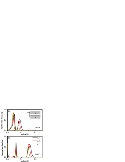
Figure 7: (color online) Spectral heat flux for graphene sheets placed on top of substrates with permittivity $\varepsilon_{s}$, where the thickness of the substrates is semi-infinite. The magnetic fields are (a) 4 T and (b) 15 T, respectively. Other parameters are kept the same as those in Fig. 3.

Technically, suspended graphene sheets can be realized in the experiments Mey:07 ; Bol:08 . However, graphene sheets are generally deposited on a variety of different substrates Edw:13 . The substrate effect for NFRHT is demonstrated in Figs. 7(a) and 7(b). As the permittivity of the dielectric substrate (non-polar and non-dispersive materials) $\varepsilon_{s}$ increases, all spectral peaks undergo a red shift. Besides, the amplitudes of the second spectral band for B=4 T and the middle spectral band for B=15 T decrease accordingly. It is expected that the substrate effect can be diminished as the thickness of substrates is reduced. Nevertheless, the multi-band spectra still persist even the substrates are taken into account. Finally, it is worth mentioning that the type of doping (electron or hole doping) in graphene could determine the sign of Hall conductivity $\sigma_{H}$. The sign of $\sigma_{H}$ is important for some remarkable phenomena such as quantum Casimir effect Tse:12 and Faraday rotation Cra:11 . However, the sign of $\sigma_{H}$ has little effect for NFRHT since the magneto-plasmon of graphene is dominant by the longitudinal component of conductivities.

IV Conclusions

In summary, magnetically tunable multi-band NFRHT is revealed in a system of two suspended graphene sheets. The single-band spectra for B=0 can be modulated greatly in the presence of a sufficient strong magnetic-field. Dual-band spectra can be realized for moderate magnetic fields (e.g., B=4 T). One band is determined by intra-band transitions in the classical regime, which undergoes a blue shift as the chemical potential increases. The other band is contributed by inter-band LL transition E${}_{0}\rightarrow$E₁ in the quantum regime, showing a robust feature against the change of chemical potential. On the other hand, triple-band spectra can be found under a strong magnetic field (e.g., B=15 T). Remarkably, there is an extremely low-frequency band with the resonant peak appearing at microwave regime, stemming from the magneto-plasmon zero modes. The performances of NFRHT due to the scattering rate, separation distance and substrate effect are demonstrated as well. Although the magnetic field considered in our work is static, it can indeed be time-dependent such as sin-cos, sawtooth, square-wave etc. As a result, a dynamic tunable multi-band NFRHT would be possible under a time-dependent magnetic field, providing a possibility for multi-band information transfer.

- (1) A. Fiorino, L. Zhu, D. Thompson, R. Mittapally, P. Reddy and E. Meyhofer, Nat. Nanotechnol. , 806-811 (2018).
- (2) B. Zhao, K. Chen, S. Buddhiraju, G. Bhatt, M. Lipson, S. Fan, Nano Energy , 344-350 (2017).
- (3) S. Basu, Z. M. Zhang, and C. J. Fu, Int. J. Energy Res. , 1203-1232 (2009).
- (4) P. B.-Abdallah and S.-A. Biehs, Z. Naturforsch. A (2), 151-162 (2017).
- (5) P. B.-Abdallah and S.-A. Biehs, Phys. Rev. B , 241401(R) (2016).
- (6) K. Joulain, J.-P. Mulet, F. Marquier, R. Carminati, and J.-J. Greffet, Surf. Sci. Rep. , 59 (2005).
- (7) S. V. Boriskina, J. K. Tong, Y. Huang, J. Zhou, V. Chiloyan, G. Chen, Photonics , 659-683 (2015).
- (8) S. Shen, A. Narayanaswamy and G. Chen, Nano Lett. (8), 2909-2913(2009).
- (9) B. Song, Y. Ganjeh, S. Sadat, D. Thompson, A. Fiorino, V. Fernández-Hurtado, J. Feist, F. J. Garcia-Vidal, J. C. Cuevas, P. Reddy and E. Meyhofer, Nat. Nanotechnol. , 253-258 (2015).
- (10) A. I. Volokitin and B. N. J. Persson, Rev. Mod. Phys. , 1291 (2007).
- (11) X. Liu, L. Wang, and Z. M. Zhang, Nanosc. Microsc. Therm. , 98-126 (2015).
- (12) J. C. Cuevas, and Francisco J. Garcia-Vidal, ACS Photonics (10), 3896-3915 (2018).
- (13) N. Li, J. Ren, L. Wang, G. Zhang, P. Hnggi, B. Li , Rev. Mod. Phys. (3), 1045 (2012).
- (14) C. R. Otey, W. T. Lau, and S. Fan, Phys. Rev. Lett. , 154301(2010).
- (15) V. Kubytskyi, S.-A. Biehs, and P. B.-Abdallah, Phys. Rev. Lett. , 074301 (2014).
- (16) K. Ito, K. Nishikawa, and H. Iizuka, Appl. Phys. Lett. , 053507 (2016).
- (17) P. B.-Abdallah and S.-A. Biehs, Phys. Rev. Lett. , 044301(2014).
- (18) O. Ilic, N. H. Thomas, T. Christensen, M. C. Sherrott, M. Soljai, A. J. Minnich, O. D. Miller, and H. A. Atwater, ACS Nano (3), 2474-2481(2018).
- (19) Y. Huang, S. V. Boriskina, G. Chen. Appl. Phys. Lett., 244102 (2014).
- (20) L. Cui, Y. Huang, J. Wang, and K.-Y. Zhu, Appl. Phys. Lett. , 053106 (2013).
- (21) J. Kou and A. J. Minnich, Opt. Express , A729-A736 (2018).
- (22) P. B.-Abdallah, Phys. Rev. Lett. , 084301 (2016).
- (23) L. Zhu, and S. Fan, Phys. Rev. Lett. , 134303 (2016).
- (24) R. M. Ab. Ekeroth, P. B.-Abdallah, J. C. Cuevas, and A. García-Martín, ACS Photonics , 705-710 (2018).
- (25) E. Moncada-Villa, V. Fernndez-Hurtado, F. J. García-Vidal, A. García-Martín, and J. C. Cuevas, Phys. Rev. B , 125418 (2015).
- (26) P. J. van Zwol, K. Joulain, P. B.-Abdallah, J. J. Greffet, and J. Chevrier, Phys. Rev. B , 201404(R) (2011).
- (27) P. J. van Zwol, L. Ranno, and J. Chevrier, Phys. Rev. Lett. , 234301 (2012).
- (28) A. Ghanekar, M. Ricci, Y. Tian, O. Gregory, and Y. Zheng, Appl. Phys. Lett. , 241104 (2018).
- (29) B. Hu, Y. Zhang and Q. J. Wang, Nanophotonics , 383-396 (2015).
- (30) J. J. Brion, R. F. Wallis, A. Hartstein and E. Burstein, Phys. Rev. Lett. , 1455 (1972).
- (31) A. Ferreira, N. M. R. Peres, and A. H. Castro Neto, Phys. Rev. B , 205426 (2012).
- (32) B. Hu, J. Tao, Y. Zhang, and Q. J. Wang, Opt. Express , 21727 (2014).
- (33) A. K. Geim and K. S. Novoselov, Nat. Mater. , 183 (2007).
- (34) M. O. Goerbig, Rev. Mod. Phys. , 1193 (2011).
- (35) Y. Zhang, Z. Jiang, J. P. Small, M. S. Purewal, Y.-W. Tan, M. Fazlollahi, J. D. Chudow, J. A. Jaszczak, H. L. Stormer, and P. Kim, Phys. Rev. Lett. , 136806 (2006).
- (36) V. P. Gusynin, S. G. Sharapov, and J. P. Carbotte, J. Phys.: Condens. Matter , 026222 (2007).
- (37) A. Ferreira, J. Viana-Gomes, Yu. V. Bludov, V. Pereira, N. M. R. Peres, and A. H. Castro Neto, Phys. Rev. B , 235410 (2011).
- (38) S. A. Biehs, P. Ben-Abdallah, F. S. S. Rosa, K. Joulain, and J.-J.Greffet, Opt. Express , A1088 (2011).
- (39) O. V. Kotov and Yu. E. Lozovik, Phys. Rev. B , 235403 (2017).
- (40) W.-K. Tse and A. H. MacDonald, Phys. Rev. Lett. , 236806 (2012).
- (41) D. Jin, L. Lu, Z. Wang, C. Fang, J. D. Joannopoulos, M. Soljai, L. Fu and N. X. Fang, Nat. Commun. , 13486 (2016).
- (42) A. N. Grigorenko, M. Polini and K. S. Novoselov, Nat. Photonics , 749-758 (2012).
- (43) O. Ilic, M. Jablan, J. D. Joannopoulos, I. Celanovic, H. Buljan, and M. Soljai, Phys. Rev. B , 155422 (2012).
- (44) I. Crassee, J. Levallois, A. L. Walter, M. Ostler, A. Bostwick, E. Rotenberg, T. Seyller, D. van der Marel and A. B. Kuzmenko, Nat. Phys. , 48-51 (2011).
- (45) J. C. Meyer, A. K. Geim, M. I. Katsnelson, K. S. Novoselov, T. J. Booth and S. Roth, Nature , 60-63 (2007).
- (46) K. I. Bolotin, K. J. Sikes, Z. Jiang, M. Klima, G. Fudenberg, J. Hone, P. Kim and H. L. Stormer, Solid State Commun. , 351-355 (2008).
- (47) R. S. Edwards and K. S. Coleman, Nanoscale , 38 (2013).