Long-range prisoner’s dilemma game on a cycle

Abstract

We investigate evolutionary dynamics of altruism with long-range interaction on a cycle. The interaction between individuals is described by a simplified version of the prisoner’s dilemma (PD) game in which the payoffs are parameterized by $c$, the cost of a cooperative action. In our model, the probabilities of the game interaction and competition decay algebraically with $r_{AB}$, the distance between two players $A$ and $B$, but with different exponents: That is, the probability to play the PD game is proportional to $r_{AB}^{-\alpha}$. If player $A$ is chosen for death, on the other hand, the probability for $B$ to occupy the empty site is proportional to $r_{AB}^{-\beta}$. In a limiting case of $\beta\to\infty$, where the competition for an empty site occurs between its nearest neighbors only, we analytically find the condition for the proliferation of altruism in terms of $c_{\mbox{\scriptsize th}}$, a threshold of $c$ below which altruism prevails. For finite $\beta$, we conjecture a formula for $c_{\mbox{\scriptsize th}}$ as a function of $\alpha$ and $\beta$. We also propose a numerical method to locate $c_{\mbox{\scriptsize th}}$, according to which we observe excellent agreement with the conjecture even when the selection strength is of considerable magnitude.

I Introduction

As Charles Darwin remarked in On the Origin of Species, “Natural selection will never produce in a being anything injurious to itself, for natural selection acts solely by and for the good of each.” The existence of altruism is seemingly at odds with this statement, as far as altruists are defined as those who benefit others at the cost to themselves. For this reason, there have been extensive studies to explain the evolution of altruism. The explanations can be categorized (arguably) into five rules, i.e., direct reciprocity, indirect reciprocity, spatial reciprocity, kin selection, and group selection Nowak (2006); Nowak et al. (2010); *abbot2011inclusive; *marshall2011group. An essential common factor in these mechanisms is the assortment of individuals carrying the cooperative phenotype Fletcher and Doebeli (2009); *park2012emergence; Débarre et al. (2014). Let us consider a population of defectors. If there emerges a group within which the members cooperate themselves, its size will increase because the members earn higher fitness than the population average. Furthermore, if the assortment can be maintained while the size of the group grows, the whole population will become cooperative. On the other hand, if the assortment breaks, making every individual interact with every other, cooperators will disappear because they earn less than the population average by construction.

Considering that the defectors always win in the mean-field regime, one may expect that spatial reciprocity becomes weaker as the dimensionality of the space $d$ increases. The logic goes as follows: In a population of size $N$, the average chemical distance between a pair of individuals behaves as $\sim N^{1/d}$ and thus decreases dramatically as $d$ grows. Hence, it is reasonable to expect a relatively homogeneous state in a high-dimensional structure. In many statistical-physical models, the mean-field theory becomes exact as $d$ exceeds a certain value $d_{c}$Landau and Lifshitz (1980). Another way to look at the crossover between a low-dimensional spin system and the mean-field limit is to consider long-range interactions on a one-dimensional (1D) lattice structure Thouless (1969); *fisher1972critical; *luijten2000monte. For example, when the interaction strength decays as $r^{-1-\sigma}$ between a pair of 1D Ising spins with distance $r$, the spins show the mean-field-like critical behaviors for $0<\sigma\leq 1/2$ as those with short range interactions in high dimensions $d>d_{c}=4$ do. For $1/2\leq\sigma\leq 1$, 1D Ising spin system shows the order-disorder transitions at finite temperatures but its critical behaviors are different from mean-field transition. For $\sigma>1$, the interactions become short-ranged effectively and they behave as the 1D spins with finite-range interactions.

The story becomes more complicated when it comes to evolutionary games: Let us consider the Prisoner’s Dilemma (PD) game with the death-birth (DB) reproduction process in the weak selection limit. It has a certain population structure, and the game is played between players at one step away. On regular structures, the condition for cooperation turns out to be determined by the number of nearest neighbors regardless of $d$ Ohtsuki et al. (2006) (see also Ref. Allen et al., 2017 for more general results). Furthermore, spatial reciprocity breaks down for any population structures if we employ the birth-death (BD) process instead. What is the difference between the DB and BD processes? The point is that we actually have another kind of interaction, that is, competition for reproduction. For social behavior to evolve, these two should have different length scales Débarre et al. (2014). Even if the game interaction shares the same underlying structure with competition for reproduction, the DB process naturally separates the scales because the competition for reproduction effectively occurs between players at two steps away.

In this paper, we wish to investigate the roles of these two length scales explicitly by considering the PD game on a cycle with long-range interactions, whose dynamics is governed by the DB process. The game is parameterized by the cost of cooperation, denoted by $c$. We are interested in its threshold, $c_{\mbox{\scriptsize th}}$, above which cooperators are outnumbered by defectors in the infinite population with zero mutation limit. The length scale of the game interaction is determined by an exponent $\alpha$, so that the game result between two individuals at distance $r$ has a weighting factor of $r^{-\alpha}$. On the other hand, the length scale of competition for reproduction is determined by another exponent $\beta$, so the probability for an individual to occupy an empty site at distance $r$ decays algebraically as $r^{-\beta}$. Our first main result is to derive $c_{\mbox{\scriptsize th}}$ for $\beta\to\infty$, where only the nearest neighbors compete for reproduction. Then, we consider the case of $\alpha=\beta$, where an analytic result for $c_{\mbox{\scriptsize th}}$ is available in the weak-selection limit Allen et al. (2017). Based on these two special cases, we conjecture a general form of $c_{\mbox{\scriptsize th}}(\alpha,\beta)$. It agrees well with numerical results.

This work is organized as follows: In the next section, we give a detailed description of our model. In Sec. III, we present $c_{\mbox{\scriptsize th}}$ as a function of $\alpha$ in case of $\beta\to\infty$ and review the exact $c_{\mbox{\scriptsize th}}$ when $\alpha=\beta$ in the weak-selection limit. Based on these two results, we conjecture $c_{\mbox{\scriptsize th}}$ for general $\alpha$ and $\beta$. Section IV compares this conjecture with Monte Carlo data. The conjectured threshold nicely matches with our numerical calculation, and this holds even if the selection strength increases. We discuss this finding and conclude this work in Sec. V.

II Model

The population structure is a cycle, i.e., a 1D lattice with the periodic boundary condition. For the sake of convenience, the total number of sites is assumed to be an add number in this section and we set $N\equiv 2n+1$. Of course, it will be irrelevant whether $N$ is even or odd if we deal with a sufficiently large system. Every site $i$ is occupied by a player, who is also denoted by $i=-n$, $-n+1$, $\ldots,-1,0,1,\ldots,n-1,n$, and each player $i$ can choose an action $s_{i}$ between cooperation $C$ and defection $D$. The PD game is formulated as the donation game, where a cooperator benefits the co-player by an amount of $b>0$ with paying cost $c\in(0,b)$. The payoff matrix $\pi$ is thus defined as

$$\begin{array}[]{cc}&\ \ \begin{array}[]{cc}\mbox{}\hskip 5.69054ptC&\mbox{}\hskip 11.38109pt\ D\end{array}\\ \begin{array}[]{c}C\\ D\end{array}&\left(\begin{array}[]{cc}b-c&\mbox{}\hskip 5.69054pt-c\\ b&0\end{array}\right).\end{array}$$ (8)

Without loss of generality, we will set $b=1$ throughout this work. The expected payoff of player $i$ per game is given by the following weighted sum,

$$\Pi_{i} = \sum_{j\not=i}\frac{r_{\!{}_{ij}}^{-\alpha}}{2\zeta_{n}(\alpha)}\pi_{s_{i}s_{j}}\ =\ \frac{1}{2\zeta_{n}(\alpha)}\sum_{j\not=i}\frac{\pi_{s_{i}s_{j}}}{r_{\!{}_{ij}}^{\alpha}}$$ (9)

where $\zeta_{n}(\alpha)\equiv\sum_{k=1}^{n}k^{-\alpha}$ is the incomplete Riemann zeta function and $r_{\!{}_{ij}}^{-\alpha}/2\zeta_{n}(\alpha)$ is the probability that player $i$ play a game with player $j$ where $r_{\!{}_{ij}}$ is the distance between them. On a cycle, $r_{\!{}_{ij}}$ is given by the minimum of $|i-j|$, $|i-j+N|$, and $|i-j-N|$. We consider the expected payoff per game (rather than the total payoff, $\sum_{j\not=i}r_{\!{}_{ij}}^{-\alpha}\pi_{s_{i}s_{j}}$) to make the average payoff independent of the population size. This normalized payoff is also better to compare two systems with different $\alpha$ fairly. The systems with smaller $\alpha$ would show effectively more strong selections without the normalization.

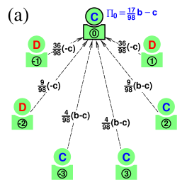
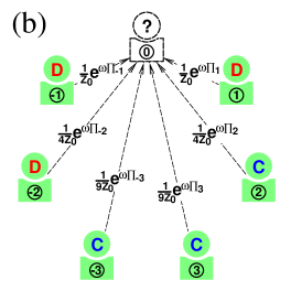
Figure 1: (Color online) Schematic representation of an example of the model ($\alpha=\beta=2$, $n=3$). (a) Payoff of the player 0. Player $0$ plays the PD game of Eq.  (8) with player $k\not=0$ producing $\pi_{0k}=b-c$ for $k=-3$, 2, and 3 and $\pi_{0k}=-c$ for $k=-2,-1$ and $1$. $\Pi_{0}$ is the weighted sum of these values with the weighting factors, $\frac{|k|^{-2}}{2\zeta_{3}(2)}$. Weighting factors are $\frac{36}{98}$ for $n=\pm 1$, $\frac{9}{98}$ for $n=\pm 2$, and $\frac{4}{98}$ for $n=\pm 3$, and Payoff of the player 0 is $\Pi_{0}=\frac{17}{98}b-c$. Payoff $\Pi_{k}$ of player $k\not=0$ can be obtained similarly; $\Pi_{-3}=\frac{49}{98}b-c$, $\Pi_{-2}=\frac{58}{98}b$, $\Pi_{-1}=\frac{53}{98}b$, $\Pi_{1}=\frac{85}{98}b$, $\Pi_{2}=\frac{54}{98}b-c$, $\Pi_{3}=\frac{49}{98}b-c$. (b) Competition for reproduction. When a player, say, $i=0$, is chosen for death, the other players $k\not=0$ compete to produce their offspring at this empty site. Player $k$’s winning probability is proportional to its fitness $f_{k}=e^{\omega\Pi_{k}}$ and inverse square distance $|k|^{-2}$. Note that $1/Z_{0}$ is to normalize the total sum of probabilities. The winner’s offspring inherits the winner’s strategy with probability $(1-\mu)$ or the opposite one with $\mu\ll 1$.

Fig. 1(a) illustrates the way to calculate payoff $\Pi_{0}$ of player 0 for $\alpha=2$ and $n=3$. Player $0$ at the top plays the PD game with every other in the population, $k=\pm 3$, $\pm 2$, and $k=\pm 1$. From Eq. (8), we see that $\pi_{0k}$ is $-c$ for $k=-2,-1$ and $1$ and $b-c$ for $k=-3$, 3, and 2. $\Pi_{0}$ is the weighted sum of these values with the wighting factors, $\frac{|k|^{-2}}{2\zeta_{3}(2)}$ where $2\zeta_{3}(2)=2\left[{1/1^{2}+1/2^{2}+1/3^{2}}\right]=\frac{98}{36}$. Since $\frac{|k|^{-2}}{2\zeta_{3}(2)}$ is $\frac{36}{98}$ for $n=\pm 1$, $\frac{9}{98}$ for $n=\pm 2$, and $\frac{4}{98}$ for $n=\pm 3$, $\Pi_{0}$ is given by $\pi_{0}=\frac{17}{98}b-c$. We can calculate the payoffs of the other players similarly. They are $\Pi_{-3}=\frac{49}{98}b-c$, $\Pi_{-2}=\frac{58}{98}b$, $\Pi_{-1}=\frac{53}{98}b$, $\Pi_{1}=\frac{85}{98}b$, $\Pi_{2}=\frac{54}{98}b-c$, $\Pi_{3}=\frac{49}{98}b-c$.

Player $i$’s fitness is given by the exponential form of the payoff,

$$f_{i} = e^{\omega\Pi_{i}},$$ (10)

where the selection strength $\omega$ represents how strongly the fitness depends on the payoff. Exponential fitness of Eq. (10) becomes the usual linear fitness of $1+\omega\Pi_{i}$ in the weak selection limit. It has an advantage over linear fitness in the strong selection limit. We can interpret the exponential fitness as fecundity directly even when the payoff is negative. Furthermore, DB dynamics is invariant under the addition of a constant to all elements in the pay off matrix which certainly preserve the Nash equilibrium.

We employ a long-range version of the DB process as a model of reproduction. The first step is to choose a death site $k$ randomly, irrespective of fitness, and make it empty. The probability to choose a particular site $k$ is therefore inversely proportional to $N$. The difference from the usual DB process for the nearest-neighbor competition is that any player $i$ in the population can produce an offspring at the empty site. For given $k$, the conditional probability $p_{ik}$ that player $i$’s offspring takes over the site $k$ is proportional to the player’s fitness $f_{i}$ but decreases as $r_{ik}^{-\beta}$ where $r_{ik}$ is the distance between them. In other words, $p_{ik}$ is given by

$$p_{ik} = \frac{1}{Z_{k}}\frac{e^{\omega\Pi_{i}}}{r_{ik}^{\beta}},$$ (11)

where $Z_{k}\equiv\sum_{i\not=k}e^{\omega\Pi_{i}}\times r_{ik}^{-\beta}$ is a normalization factor. Note that the player at the death site $k$ cannot leave an offspring. In particular, $s_{k}$ will become $C$ with probability

$$P^{0}_{s_{k}\to_{C}} = \frac{1}{Z_{k}}\,\sum_{i\not=k}\frac{e^{\omega\Pi_{i}}}{r_{ik}^{\beta}}\,\delta_{s_{i},C},$$ (12)

where $\delta_{x,y}$ is the Kronecker delta. To remove trivial absorbing states where every player takes the same action, we introduce a small mutation probability $\mu$. When player $i$ reproduces its offspring at the site $k$, $s_{k}$ becomes $s_{i}$ with probability $1-\mu$ and by the opposite of $s_{i}$ with probability $\mu$. If we combine the DB process and mutation together, the actual probability that $s_{k}$ becomes $C$ is given by

$$P_{s_{k}\to_{C}} = \left({1-\mu}\right)P^{0}_{s_{k}\to_{C}}+\mu\left({1-P^{0}_{s_{k}\to_{C}}}\right).$$ (13)

It is straightforward to see that the complementary event $s_{k}\to D$ occurs with probability $1-P_{s_{k}\to_{C}}$.

We demonstrate the reproduction process in Fig. 1(b) for $\beta=2$ and $n=3$. When a player, say, $i=0$, is chosen for death, the other players $k\not=0$ compete to produce their offspring at this empty site. Player $k$’s winning probability is given by $\frac{1}{|k|^{2}\,Z_{0}}\,e^{\omega\Pi_{k}}$ with $\Pi_{k}$ given in the caption of (a). Here $Z_{0}=e^{\omega\Pi_{1}}+e^{\omega\Pi_{-1}}+\frac{1}{4}\left[{e^{\omega\Pi_{2}}+e^{\omega\Pi_{-2}}}\right]+\frac{1}{9}\left[{e^{\omega\Pi_{3}}+e^{\omega\Pi_{-3}}}\right]$ so that the normalization factor $1/Z_{0}$ makes the total sum of probabilities be 1. The winner’s offspring inherits the winner’s strategy with probability $(1-\mu)$ or the opposite one with $\mu\ll 1$.

III Analysis

We begin by considering how the threshold cost $c_{\mbox{\scriptsize th}}(\alpha,\beta)$ behaves in special cases. The first one is the case with the nearest-neighbor competition, represented by $\beta\to\infty$. The second one is when $\alpha=\beta$, and $c_{\mbox{\scriptsize th}}(\alpha,\alpha)$ in the weak-selection limit is readily obtained by applying the result of Ref. Allen et al., 2017.

III.1 Nearest-neighbor competition ($\beta\to\infty$)

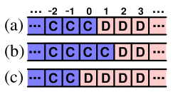
Figure 2: (Color online) Domain-wall dynamics in case of the nearest-neighbor competition ($\beta\to\infty$). (a) Initial configuration in which two domains meet at a wall between the sites $k=0$ and $1$. The competition for reproduction occurs between the players at these sites. (b) If $k=1$ is made empty and occupied by an offspring of the player at $k=0$, the domain wall moves right. (c) On the contrary, the domain wall moves left if $k=0$ is made empty and taken over by an offspring of the player at $k=1$.

If $\beta\to\infty$, only the nearest neighbors of the death site will compete for reproduction. Let us define a domain as a set of consecutive sites with the same action, bounded by sites with the opposite action. When a death site $k$ is picked up inside a domain, therefore, the action of its neighbors must be the same as $s_{k}$. If $\mu$ is negligibly small, we can say that the configuration $\left\{s_{i}\right\}$ will not change. It implies that the system shows dynamics only at domain boundaries. Let us assume that the system is divided into two equally large domains so that

$$s_{i}=\left\{\begin{array}[]{lcl}C&\text{for}&i=0,-1,-2,\ldots,-n\\ D&\text{for}&i=1,2,\ldots,n,\end{array}\right.$$ (14)

as shown in Fig. 2(a). Assume that $k=1$ is chosen as for death. Only its neighboring players $k=0$ and $k=2$ compete to take over the empty site, and the domain wall will move right if the offspring of player $i=0$ wins. The payoffs $\Pi_{0}$ and $\Pi_{2}$ are calculated as

$$\Pi_{0} = \frac{1}{2\zeta_{n}(\alpha)}\sum_{j\not=0}\frac{\pi_{s_{0}s_{j}}}{r_{0j}^{\alpha}}$$ (15)

$$= \frac{1}{2\zeta_{n}(\alpha)}\sum_{r=1}^{n}\left({\frac{1-c}{r^{\alpha}}+\frac{-c}{r^{\alpha}}}\right)\ =\ \frac{1}{2}-c,$$

$$\Pi_{2} = \frac{1}{2\zeta_{n}(\alpha)}\sum_{j\not=2}\frac{\pi_{s_{2}s_{j}}}{r_{2j}^{\alpha}}$$ (16)

$$= \frac{1}{2\zeta_{n}(\alpha)}\sum_{r=2}^{n}\frac{1}{r^{\alpha}}\ =\ \frac{1}{2}-\frac{1}{2\zeta_{n}(\alpha)},$$

and the probability that the wall moves right is given by

$$P^{0}_{s_{1}\to C} = \frac{e^{\omega\Pi_{0}}}{e^{\omega\Pi_{0}}+e^{\omega\Pi_{2}}}.$$ (17)

Similarly, we can calculate the probability that the wall moves left, $P^{0}_{s_{0}\to D}$, from $\Pi_{-1}$ and $\Pi_{1}$. The population will become cooperative when $P^{0}_{s_{1}\to C}>P^{0}_{s_{0}\to D}$. If $N\gg 1$, this inequality reduces to

$$c<\frac{1}{2\zeta_{n}(\alpha)}$$ (18)

and we have $c_{\mbox{\scriptsize th}}(\alpha,\infty)=1/2\zeta_{n}(\alpha)$.

III.2 Analytic solution of $\alpha=\beta$

If the game interaction and competition share the same population structure, strategies selected by the network reciprocity can be obtained on any population structure in the weak-selection limit of $\omega\to 0$ using coalescent theory Allen et al. (2017). When we denote the expected coalescence time Wakeley (2008) from the two ends of an $n$-step random walk by $\tau_{n}$, cooperation is favored when $c$ is smaller than

$$c_{\mbox{\scriptsize th}}=\frac{\tau_{3}-\tau_{1}}{\tau_{2}}$$ (19)

in the weak-selection limit. In a weighted undirected graph, if site $i$ is connected to $j$ by an edge, the edge has a weight $w_{ij}=w_{ji}$. The weighted degree of site $i$ is the sum of its edge weights: $w_{i}\equiv\sum_{j}w_{ij}$. The probability for a random walker to transit from $i$ to $j$ is denoted by $p_{ij}\equiv w_{ij}/w_{i}$. A useful quantity is the Simpson degree $\kappa_{i}=\left(\sum_{j}p_{ij}^{2}\right)^{-1}$, a generalization of the topological degree. For a regular graph, the site index $i$ is unnecessary since every vertex has the same Simpson degree $k_{i}=k$. Equation (19) is then rewritten as

$$c_{\mbox{\scriptsize th}}=\frac{N/\kappa-2}{N-2}.$$ (20)

In our case, noting that $w_{ij}\propto r_{ij}^{-\alpha}$ for $i\neq j$ and $w_{ii}=0$, we find the threshold as a combination of the zeta functions Hardy and Wright (1979),

$$c_{\mbox{\scriptsize th}}(\alpha,\alpha)=\frac{\zeta_{n}(2\alpha)}{2\left[{\zeta_{n}\left({\alpha}\right)}\right]^{2}},$$ (21)

where we have taken into account $N\gg 1$ in the sense of the $\omega N$-limit Jeong et al. (2014).

III.3 Conjecture for $c_{\mbox{\scriptsize th}}(\alpha,\beta)$

To recap, we have two predictions: First, if $\beta\to\infty$ and $N\gg 1$, the threshold cost is predicted to be

$$c_{\mbox{\scriptsize th}}(\alpha,\infty)=\frac{1}{2\zeta_{n}(\alpha)},$$ (22)

so that $\zeta_{n}(\alpha)$ can be interpreted as the effective number of neighbors to play the game with on one side of the focal player. Second, when $\alpha=\beta$, the threshold cost $c_{\mbox{\scriptsize th}}$ has been derived as

$$c_{\mbox{\scriptsize th}}(\alpha,\alpha)=\frac{\zeta_{n}(\alpha+\alpha)}{2\zeta_{n}(\alpha)\zeta_{n}(\alpha)}$$ (23)

for $\omega\to 0$. To incorporate Eqs. (22) and (23), we conjecture a connection formula $c_{\mbox{\scriptsize th}}(\alpha,\beta)$ as follows:

$$c_{\mbox{\scriptsize th}}(\alpha,\beta)=\frac{\zeta_{n}(\alpha+\beta)}{2\zeta_{n}(\alpha)\zeta_{n}(\beta)}.$$ (24)

In particular, for $\alpha\to\infty$, the conjecture predicts

$$c_{\mbox{\scriptsize th}}(\infty,\beta)=\frac{1}{2\zeta_{n}(\beta)}.$$ (25)

IV Numerical calculation

For Monte Carlo simulation, we construct a cycle of size $N$ with a player at each site. Initial $s_{i}$’s are randomly chosen between $C$ and $D$ equally probably. Then, according to the DB process, we randomly select a player (say, $k$) for death and choose another player $i$ with probability $p_{ik}$ in Eq. (11). One Monte Carlo step consists of $N$ trials to update the configuration $\{s_{i}\}$. In addition, we introduce mutation with small probability $\mu\ll 1$ so that the system has a unique stationary distribution over configurations $\left\{s_{i}\right\}$. The quantity of interest is cooperator abundance $x_{\!{}_{C}}$, the average frequency of cooperators in the steady state. For each data point in a sample, we run the Monte Carlo simulation for $6\times 10^{3}$ Monte Carlo steps, and the time average of $x_{\!{}_{C}}$ is taken for the last $10^{2}$ Monte Carlo steps, at which the simulation has already reached a steady state. The total number of samples amounts to $4\times 10^{3}$.

IV.1 Weak selection ($w=0.02$)

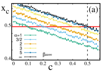
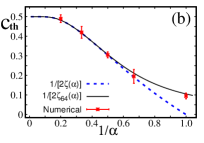
Figure 3: (Color online) Threshold estimation in case of nearest-neighbor competition ($\beta\to\infty$). The parameters for Monte Carlo simulation are the total number of sites $N=128$, selection strength $\omega=0.02$, and mutation rate $\mu=10^{-3}$. (a) Cooperator abundance $x_{\!{}_{C}}$ as a function of $c$ for each different $\alpha$. The vertical dotted line means $c=1/2$, and the horizontal shaded area represents $0.495\pm 0.001$, the error-bar range of $x_{\!{}_{C}}(c=1/2)$ for $\alpha\to\infty$. (b) The error-bars show $[c_{\min},c_{\max}]$ for different values of $\alpha$. The solid line depicts our analytic threshold in Eq. (22) for $N=128$, and the dotted line shows the limit of $N\to\infty$.

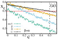
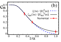
Figure 4: (Color online) Threshold estimation for $\alpha=\beta$. The simulation parameters are the same as in Fig. 3. (a) Cooperator abundance $x_{\!{}_{C}}$ as a function of $c$ for each different $\alpha$. The vertical dotted line means $c=1/2$, and the horizontal shaded area represents $0.495\pm 0.001$, the error-bar range of $x_{\!{}_{C}}(c=1/2)$ for $\alpha\to\infty$. (b) The error-bars show $[c_{\min},c_{\max}]$ for different values of $\alpha$. The solid line depicts our analytic threshold in Eq. (23) for $N=128$, and the dotted line shows the limit of $N\to\infty$.

Noting that most of the analytic results have been obtained in the weak-selection limit, we have to check this limit first and proceed to stronger selection strengths thereafter. Let us begin by setting $\beta\to\infty$. If $\alpha$ also goes to infinity, the threshold at which $x_{\!{}_{C}}(c_{\mbox{\scriptsize th}})=1/2$ is analytically given as $c_{\mbox{\scriptsize th}}(\infty,\infty)=1/2$ in the $\omega N$-limit Jeong et al. (2014). However, this limit cannot be taken exactly in the Monte Carlo simulation, and $\mu$ cannot be infinitesimally small either. For $c=1/2$, we actually observe $x_{\!{}_{C}}=0.495\pm 0.001$. We regard this value as a reference point to estimate $c_{\mbox{\scriptsize th}}(\alpha,\infty)$, assuming that it takes into account all the corrections due to the difference from the $\omega N$-limit as well as the finiteness of $\mu$. The procedure to estimate $c_{\mbox{\scriptsize th}}(\alpha,\infty)$ now goes as follows: For given $\alpha$, we calculate $x_{\!{}_{C}}$ as a function of $c$, together with the standard error from statistically independent samples. As a lower bound of $c_{\mbox{\scriptsize th}}(\alpha,\infty)$, we pick up $c_{\min}$, defined as $c$ below which all the error bars of $x_{\!{}_{C}}(c)$ lie above $0.495\pm 0.001$. Likewise, the upper bound of $c_{\mbox{\scriptsize th}}(\alpha,\infty)$ is given by $c_{\max}$, defined as $c$ above which all the error bars of $x_{\!{}_{C}}(c)$ lie below $0.495\pm 0.001$ [Fig. 3(a)]. The numerical estimate of $c_{\mbox{\scriptsize th}}(\alpha,\infty)$ is thus represented by an interval $[c_{\min},c_{\max}]$ as shown in Fig. 3(b). The agreement with Eq. (22) is compelling. The above procedure can be applied to the case of $\alpha=\beta$ as well [Fig. 4(a)]. Here, the estimation is more difficult because the slope of $x_{\!{}_{C}}$ becomes steeper as $\alpha$ decreases. Nevertheless, Fig. 4(b) shows that our estimates are consistent with the analytic solution [Eq. (23)].

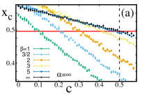
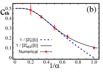
Figure 5: (Color online) Threshold estimation for $\alpha=\infty$. The simulation parameters are the same as in Fig. 3. (a) Cooperator abundance $x_{\!{}_{C}}$ as a function of $c$ for each different $\beta$. The vertical dotted line means $c=1/2$, and the horizontal shaded area represents $0.495\pm 0.001$, the error-bar range of $x_{\!{}_{C}}(c=1/2)$ for $\beta\to\infty$. (b) The error-bars show $[c_{\min},c_{\max}]$ for different values of $\beta$. The solid line depicts our conjectured threshold in Eq. (25) for $N=128$, and the dotted line shows the limit of $N\to\infty$.

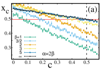
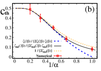
Figure 6: (Color online) Threshold estimation for $\alpha=2\beta$. The simulation parameters are the same as in Fig. 3. (a) Cooperator abundance $x_{\!{}_{C}}$ as a function of $c$ for each different $\beta$. The vertical dotted line means $c=1/2$, and the horizontal shaded area represents $0.495\pm 0.001$, the error-bar range of $x_{\!{}_{C}}(c=1/2)$ for $\beta\to\infty$. (b) The error-bars show $[c_{\min},c_{\max}]$ for different values of $\beta$. The solid line depicts our conjectured threshold in Eq. (24) for $N=128$, and the dotted line shows the limit of $N\to\infty$. For comparison, we have also plotted $1/[2\zeta_{64}(\beta)]$ as in Fig. 5(b), which deviates from the numerical data.

Let us move on to check whether the conjecture of Eq. (24) correctly predicts the threshold behavior even when no analytic proof is available. One specific example that we can test is an extreme case of $\alpha\to\infty$, where the conjecture reduces to Eq. (25). Comparing Fig. 5(a) with Fig. 3(a), we see that $\alpha$ and $\beta$ do not play the same role in determining the cooperator abundance. Nevertheless, Fig. 5(b) substantiates the conjectured symmetry between $\alpha$ and $\beta$ in the threshold behavior. To make both $\alpha$ and $\beta$ finite yet unequal, we consider another case of $\alpha=2\beta$ [Fig. 6(a)]. Again, our numerical results support the conjecture in Eq. (24). The overall behavior might look similar to the previous case of $\alpha=\infty$, but a closer look shows that our numerical estimates are sharp enough to distinguish the difference between them [Fig. 6(b)].

IV.2 Stronger selection ($w=1$ and $w=5$)

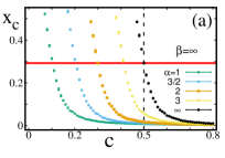
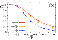
Figure 7: (Color online) Threshold estimation for $w=1$. The other simulation parameters are the same as in Fig. 3. (a) Cooperator abundance $x_{\!{}_{C}}$ as a function of $c$ for each different $\alpha$, while $\beta\to\infty$. The vertical dotted line means $c=1/2$, and the horizontal shaded area represents $0.2923\pm 0.0045$, the error-bar range of $x_{\!{}_{C}}(c=1/2)$ for $\alpha\to\infty$. (b) The error-bars show $[c_{\min},c_{\max}]$ for different values of $\beta$. The lines depict our conjectured thresholds in Eq. (24).

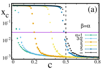
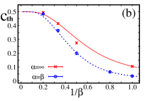
Figure 8: (Color online) Threshold estimation for $w=5$. The other simulation parameters are the same as in Fig. 3. (a) Cooperator abundance $x_{\!{}_{C}}$ as a function of $c$ for each different $\alpha=\beta$. The vertical dotted line means $c=1/2$, and the horizontal shaded area represents $0.0280\pm 0.0007$, the error-bar range of $x_{\!{}_{C}}(c=1/2)$ for $\alpha\to\infty$. Note the logarithmic scale on the vertical axis. (b) The error-bars show $[c_{\min},c_{\max}]$ for different values of $\beta$. The lines depict our conjectured thresholds in Eq. (24).

The conjectured formula [Eq. (24)] works even beyond the weak-selection limit. Our numerical estimation procedure hinges on the fact that we can still take $c=1/2$ as the threshold in a double limit of $\alpha\to\infty$ and $\beta\to\infty$ for arbitrary selection strength Jeong et al. (2014). In this limit, our numerical calculation gives $x_{c}=0.2923\pm 0.0045$ at $c=1/2$, provided that we have set $w=1$ [Fig. 7(a)]. As we have done above, we will take this value as a reference point to locate the threshold in other combinations of $\alpha$ and $\beta$ for which one can suitably define an extrapolation to $\alpha\to\infty$ and $\beta\to\infty$: Let us take a look at the results shown in Fig. 7(b). Here, we demonstrate three cases, $\alpha=\infty$, $\alpha=2\beta$, and $\alpha=\beta$. Note that the limit can be approached by taking $\beta\to\infty$ for all these cases, so that the abundance levels may be compared with the reference value in the double limit. Although none of the cases have been solved analytically, the threshold behavior is indeed captured by Eq. (24) with high precision.

As $w$ increases, the quality of fit deteriorates, however. For $w=5$, for example, the reference value is lowered to $x_{c}=0.0280\pm 0.0007$ [Fig. 8(a)]. It is a tiny value, and the slope of $x_{\!{}_{C}}(c)$ is steep, which makes the estimate more challenging than the previous weaker-selection cases. It is not surprising that deviations from the conjecture become visible [Fig. 8(b)], but the overall agreement is still remarkable.

V Concluding remarks

To summarize, we have studied the PD game on a cycle, where the probabilities for two players at distance $r$ to play the game and to compete for reproduction decay algebraically as $r^{-\alpha}$ and $r^{-\beta}$, respectively. When the benefit of cooperation is fixed as unity, there exists a threshold cost $c_{\mbox{\scriptsize th}}(\alpha,\beta)$ below which the population becomes cooperative. Based on analytically tractable cases [Eqs. (22) and (23)], we have conjectured its functional form as given in Eq. (24). The apparent symmetry between $\alpha$ and $\beta$ in Eq. (24) is nontrivial as one sees that Fig. 3(a) clearly differs from 5(a). Although we are unable to prove our conjecture at the moment, the striking agreement with numerical results suggests that the exact result of $c(\alpha,\alpha)$ can be generalized in a simple form, at least in this particular long-ranged interaction model on a cycle.

The threshold costs in our model do not seem to depend on the selection strength $\omega$ strongly. For the nearest neighbor competitions ($\beta\to\infty$), this independence can be understood easily since the threshold cost is obtained from the domain boundary dynamics as discussed in III A. For finite $\beta$, our conjecture relies on the analytic solution of weak selection limit. However, the threshold costs are almost independent of selection strength up to $\omega\approx 5$. Further studies on the robustness of the weak selection limit as well as the threshold costs for general population structures are needed.